Electromagnetic waves propagation through an array of superconducting qubits: manifestations of non-equilibrium steady states of qubits

Let us consider a regular one-dimensional array of $N$ lumped superconducting quantum circuits embedded in a low-dissipative nondispersive transmission line (see Fig. 1). As the amplitude of propagating EWs is not too low, i.e in the regime of large number of photons, the electromagnetic field in the transmission line is characterized by coordinate and time dependent classical variables - the charge distribution, $Q(x,t)$. Different types of lumped superconducting quantum circuits have been realized (the schematics of arrays composed of charge (Fig. 1(A)) and flux (Fig. 1(B),(C)) qubits are shown), and the quantum dynamics of such circuits is characterized by quantum variables-the Josephson phases, $\varphi_{n}$. An artificially prepared potential $U(\varphi_{n})$ allows one to vary the circuits resonant frequencies in a wide region. The dynamics of a whole system in the classical regime is described by total Lagrangian, which consists of three parts: the Lagrangian of electromagnetic field $L_{EF}$, the Lagrangian of an array of lumped superconducting quantum circuits (qubits) $L_{qb}$, and the interaction Lagrangian $L_{int}$ describing the interaction between qubits and electromagnetic field:

The electromagnetic field Lagrangian $L_{EF}$ is written as

where $c_{0}=1/\sqrt{L_{0}C_{0}}$ is the velocity of EWs propagating in the transmission line, $L_{0}$ and $C_{0}$ are the inductance and capacitance of the transmission line per length, accordingly; $\ell$ is the length of the system.

The Lagrangian of an array of lumped quantum circuits is written as

where $E_{J}$, $\omega_{p}$ are the Josephson energy and the plasma frequency, accordingly; the parameter $\dot{\phi}_{0n}$ is proportional to the gate voltage, and it allows one to vary the frequency of charge qubits (such gate circuits are shown by dashed arrows in Fig. 1(A)). For charge qubits the potential $U(\varphi_{n})$ is written explicitly as $U(\varphi_{n})=E_{J}(1-\cos\varphi_{n})$ whereas for flux qubits (see Fig. 1(B),(C)) the double well potential reads as: $U(\varphi_{n})=-E_{J}[2\cos\varphi_{n}-\eta\cos(2\varphi_{n})]$.

The interaction part of the Lagrangian is written as

where the coupling coefficient $\alpha$ varies by around five order of magnitude from $10^{-2}$ for a weak coupling between qubits and transmission line Macha et al. 2014 (Fig. 1(B)) up to $4\times 10^{2}$ for strongly coupled qubits Shulga et al. 2018 (Fig. 1(C)). The $w$ is the geometrical size of lumped quantum circuits (qubits), $w\ll\ell$.

As we turn to the coherent quantum regime of networks of qubits, the dynamics of EWs is described by the specific wave equation as

where we take into account the dissipation effects in the transmission line characterized by phenomenological parameter $\gamma\ll 1$. Here, $<...>_{eq}$ denotes the quantum mechanical averaging over the equilibrium state of quantum network.

Since we neglect the direct coupling between elementary circuits, the coherent quantum dynamics of a network is reduced to the sum of independent lumped electromagnetic circuit exposed to an applied electromagnetic field. The quantum dynamics of a single element is determined by the time-dependent Hamiltonian, $\hat{H}_{qb}=\hat{H}_{0}+\hat{H}_{t}$, where the equilibrium Hamiltonian $\hat{H}_{0}$ is

and the nonequilibrium part of the total Hamiltonian, explicitly depending on time, $\hat{H}_{t}$ is

In the resonant regime as the EW frequency $\omega\simeq\omega_{q}$, we truncate the explicit Hamiltonian (see Eqs . (6) and (7)) to the Hamiltonian of two-levels systems. These two levels can be fine-tuned to the resonance with the frequency of EW propagating in the transmission line. In particular, for the charge qubits case shown in Fig. 1(A), on the avoid-crossing point such truncation leads to the effective Hamiltonian written as Pashkin et al. 2003

where $\hat{\sigma}_{x,z}$ are the Pauli matrices. In this case the qubit frequency is expressed as $\omega_{q}=E_{J}$. The time-dependent wave function of a charge qubit is written as

where $f_{\pm}=\frac{1}{\sqrt{4\pi}}\left(1\pm e^{i\varphi}\right)$ stationary wave functions of two states. The corresponding quantum-mechanical average of the operator $<\dot{\varphi}>$ in the right hand part of Eq. (5) reads as

Taking into account the initial conditions $C_{-}(0)=1$ and $C_{+}(0)=0$, and using the resonant condition, $\omega_{q}\simeq\omega$ we obtain in the non-dissipative (nd) regime

where we introduce the dimensionless strength of interaction, $\eta=\alpha[\hbar\omega_{p}/(2E_{J})]^{2}$ and the dimensionless charge distribution, $q(x,t)=Q(x,t)/e$. In the low-dissipative regime we introduce the relaxation time $T$, and by solving the dynamic equations for the density matrix, the time-dependent correlation function of $n$-th qubit is written in the following form:

Substituting (10) and (11) in (5) we obtain the effective equation allowing one to analyze the transmission coefficient $D(\omega)$ for propagating EWs of frequency $\omega$.

As the power of applied microwave radiation is low, one can neglect the nonlinear dependence of $\beta(q)$ on $q$, and by making use of a well known result for the quantum tunneling through a rectangular barrier the transmission coefficient is written as

where $K(\omega)=\frac{gc_{0}}{\omega_{q}a}\frac{(1-\omega/\omega_{q})+i\Gamma}{(1-\omega/\omega_{q})^{2}+\Gamma^{2}}$.

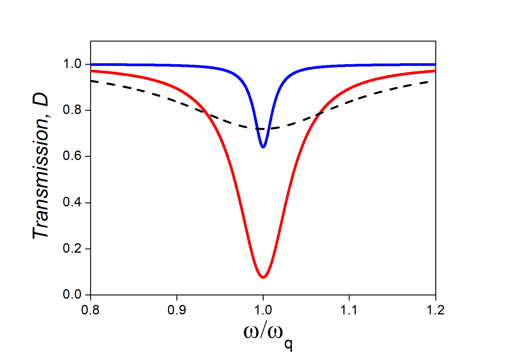
Here, we consider a regime most relevant to current experiments as the total length of a system is smaller than the wave length of EWs, i.e. $\ell\ll\lambda=c_{0}/\omega$, and the effective strength of interaction between a single qubit and EWs is large, i.e. $\beta/a\gg\omega_{q}^{2}$. With such assumptions the dependencies of $D(\omega)$ for different values of an effective strength of interaction $g$ are presented in Fig. 4. Beyond a standard resonant suppression of $D(\omega)$ observed for moderately large values of $g$ (see Fig.4, red line) , we obtain a great enhancement of $D(\omega)$ in an extremely narrow region of frequencies (see Fig.4, blue line). This effect of resonant transparency of EWs propagating through an array of qubits occurs for an extremely large values of an effective strength of interaction $g$. We notice that such resonant propagation of EWs through a chain of densely arranged superconducting qubits has been experimentally observed in Shulga et al. 2018 where an extremely large value of coupling was achieved by direct incorporation of qubits Josephson junctions in the superconducting transmission line. Moreover, as the size of the array increases we obtain a large set of peaks in the dependence of $D(\omega)$. It is shown in Fig. 5.

In the regime of high power applied microwave radiation the dynamics of EWs is determined by generic Eq. (18) written as

where $\chi=[gc_{0}/(\eta^{2}\omega_{q}a)](\omega_{q}-\omega)$ and $\xi=(1/\eta^{2})[(\omega_{q}-\omega)^{2}+\Gamma^{2}]$. Here, we neglect a small absorption of EWs, i.e. an imaginary part of $k$ and $\chi$. We solve such intrinsically nonlinear wave equation by making use of an analogy with the famous Kepler problem in classical mechanics Landau and Lifshitz 1960. To make that we introduce the spatially dependent amplitude $r(x)$ and the phase $\phi(x)$ of EWs as $q(x)=r(x)e^{i\phi(x)}$ and $|q|=r$. Spatial distributions of the amplitude $r(x)$ and phase $\phi(x)$ of the electromagnetic field are determined by following equations:

where we introduce the nonlinear function $R(r)=\frac{\chi}{r^{2}+\xi^{2}}$, $C$ is the constant that have to be found from the boundary conditions. The boundary conditions are derived from the continuity of the electric and magnetic fields of EW at the boundaries, $x=0$ and $x=\ell$, of a system. The boundary conditions are explicitly written down as

where the amplitude of incident EW, $A\propto\sqrt{P}$ and $P$ is the power of an incident EW. The transmission coefficient of propagating EWs is determined as $D=|q(\ell)/A|^{2}$. The solution of Eq. (21) is obtained as

where the constant $E$ is the effective energy of a system. The constant $C$ is determined as: $C=k[r(\ell)]^{2}$. In the limit of not extremely large coupling $g$ and large system size, $kl\gg 1$, using the condition $|r(\ell)-r(0)|\ll r(0)$ we write down the expression for the transmission coefficient $D(\omega)$ as

where the variable $z=r(0)/r(\ell)$ is closed to one. The parameter $z$ is determined by the transcendent equation derived from Eq. (23) as

Thus, the parameter $z$ is obtained explicitly as

Substituting (26) in (24) we obtain in a strongly nonlinear regime the transmission coefficient of $D(\omega)$ as

For various parameters $\omega_{q}-\omega$, $\chi$ and $\Gamma$ the dependencies of $D(P)$ are presented in Fig. 6.

Thus, the main result of this Section is that if for low power EWs the transmission $D$ is strongly suppressed ($D\ll 1$) but in the high-power limit the transmission will be recovered to $D\simeq 1$. The origin of such effect is an equalizing of the populations of qubits states in the limit of a large power of EWs, that, in turn, strongly suppresses the ac response of qubits to the applied electromagnetic field.