Robust Sound Source Localization considering Similarity of Back-Propagation Signals
Abstract
We present a novel, robust sound source localization algorithm considering back-propagation signals. Sound propagation paths are estimated by generating direct and reflection acoustic rays based on ray tracing in a backward manner. We then compute the back-propagation signals by designing and using the impulse response of the backward sound propagation based on the acoustic ray paths. For identifying the 3D source position, we suggest a localization method based on the Monte Carlo localization algorithm. Candidates for a source position is determined by identifying the convergence regions of acoustic ray paths. This candidate is validated by measuring similarities between back-propagation signals, under the assumption that the back-propagation signals of different acoustic ray paths should be similar near the sound source position. Thanks to considering similarities of back-propagation signals, our approach can localize a source position with an averaged error of 0.51 m in a room of 7 m by 7 m area with 3 m height in tested environments. We also observe 65 % to 220 % improvement in accuracy over the state-of-the-art method. This improvement is achieved in environments containing a moving source, an obstacle, and noises.
I INTRODUCTION
As robots become more widely available, it is getting more imperative for a robot to understand environments for safe and accurate operations. There have been many kinds of research efforts to perceive the environments by acquiring and using data from hardware sensors. One of main the research topics for understanding the environments focus on identifying locations of a robot itself and other objects in environments from collected data by vision cameras and depth sensors. Departing from these approaches, an acoustic data measured by acoustic sensors has recently attracted attention as an important clue for localizing various objects.
The problem identifying the location of a sound source from collected acoustic data is widely known as the sound source localization (SSL). There have been many types of SSL researches including the use of a time difference of arrival (TDOA) of sound waves at microphones [6, 14] and advanced methods using a spherical microphone array based on the analysis of the spherical harmonics functions [5, 8, 10, 15].
These approaches, unfortunately, are not designed mainly for the estimation of 3D position but for the identification of an incoming direction of sound. Especially, when a sound source is occluded by an obstacle or multiple sound sources are located in the same direction, most of prior approaches cannot specify the location of the source generating the sound signal. To address this issue, recent techniques were proposed to find a 3D source location even if the sound source is in the non-line-of-sight state [1, 2]. These techniques estimate sound propagation paths from the source to microphones as acoustic rays, generated by the ray tracing technique, and identify the 3D source location by using generated acoustic rays. However, the accuracy of these methods decreases in noisy environments including a moving sound and obstacles.

Main Contributions. To robustly identify the sound source location, we present a novel, sound source localization algorithm using back-propagation signals (Fig. 1). Using a beamforming algorithm, we first compute incoming directions of the sound and separation signals corresponding to those specific incoming directions (Sec. IV-A). We then estimate sound propagation paths by generating acoustic ray paths in the reverse direction to the incoming directions of the sound (Sec. IV-B), and compute the back-propagation signals using the impulse response of the acoustic ray path from the separation signal (Sec. IV-C). Intuitively speaking, back-propagation signals are virtually computed signals that could be heard at a particular location in acoustic paths from the measured signals at the microphone array.
Finally, we use the Monte Carlo localization algorithm estimating a location of the sound as a converging region of computed acoustic ray paths. In particular, we utilize the computed back-propagation signals of different acoustic ray paths for accurate estimation of the sound location, under the intuitive assumption that acoustic paths coming from the same sound source should have similar back-propagation signals at the estimated location (Sec. IV-D).
Given environments containing a moving source, an obstacle, and noises in a 7m7m3m room, our localization algorithm estimates the location of the sound source with an error of 0.5m on average. The localization algorithm of our approach is improved by 65%–220% compared to the prior work that does not consider the back-propagation signals.
II RELATED WORKS
In this section, we give a brief overview of prior works on sound source localization and sound propagation.
II-A Sound source localization
There has been a significant amount of efforts to localize a sound source by estimating a direction of sound. Many works have been studied based on time difference of arrival (TDOA) of a microphone array. Knapp et al. [6] suggested an efficient algorithm to estimate a time delay of sound arrivals at each microphone pair.
When the shape of the microphone array is spherical, one can uniformly estimate angle of sound sources in every azimuth and elevation angle. Therefore, many beamformer algorithms have been studied by using the spherical Fourier transform, which transforms the function on the unit sphere to the spherical harmonics domain. Rafaely [9, 11] presented a theoretical framework of analysis of spherical microphone array. This approach localized the source direction by computing the beam energy map on the unit sphere using steered beamformer algorithms. Valin et al. [14] suggested a memoryless localization algorithm based on a simple delay-and-sum beamformer on the space domain using 8 microphones located on the surface of the sphere, and Rafaely [10] extended the delay-and-sum localization method to process on the spherical harmonics domain. Yan et al. [15] suggested a localization algorithm using the minimum variance distortionless response (MVDR) power spectra on the spherical harmonics domain. Li et al. [8] presented a MUSIC (Multiple Signal Classification) based beamformer algorithm, which uses an orthogonality between a noise-only subspace and a signal-plus-noise subspace on the spherical harmonics domain. Khaykin et al. [5] presented a frequency smoothing technique for spherical microphone arrays. Unfortunately, these techniques were designed for detecting incoming directions, not the 3D location of a sound source in an arbitrary environment.
Recently, 3D sound source localization methods have emerged by considering not only the direct path, but also indirect paths such as reflection and diffraction of sound propagation. An et al. [2] suggested a reflection-aware SSL algorithm via approximating sound propagation as acoustic rays generated by a ray tracing technique. This technique was extended to a diffraction-aware localization method for handling a non-line-of-sight sound source [1]. These methods localize the 3D source position by identifying the convergence region of acoustic rays based on the hypothesis that acoustic rays are generated from the same source. However, if there exist many convergence regions of acoustic rays in environments containing a moving sound, obstacles, and noises, we observe that the accuracy deteriorates (Sec. V). In this paper, we aim to overcome this issue by utilizing the acoustic signals back-propagated to the source location.

II-B Sound propagation
For the generation of acoustic rays and back-propagation signals, an accurate sound propagation model should be employed. Various sound propagation models have been studied for generating a realistic sound in a virtual environment. For generating a realistic sound, these prior methods have focused on modeling how the sound emitted at the source is propagated to the listener.
At a broad level, sound propagation techniques can be categorized as numerical acoustic (NA) and geometric acoustic (GA) methods. NA techniques have been studied based on modeling the sound propagation using the acoustic wave equation. Since it requires considerable amount of computation time to solve the acoustic wave equation, there are difficulties in extending NA techniques to real-time applications.
GA techniques are based on ray tracing algorithms and facilitate an efficient sound simulation for real-time applications by estimating an acoustic impulse response between a source and a listener in an environment. Cao et al. [3] enabled efficient computation of sound simulation through bidirectional path tracing. Li et al. [7] proposed an efficient sound simulator for videos by handling early and late reverberation separately.
There have been hybrid approaches supporting various low-frequency wave properties within GA methods. Yeh et al. [16] presented a hybrid approach that combines geometric and numeric methods for handling complex environments. Schissler et al. [12] suggested an efficient way to deal with reverberation by considering high-order diffraction and diffuse reflection in large environments.
For improving the accuracy of sound source location, which is an inverse problem to the sound generation, we adopt the concept of an impulse response used for these sound generation methods. The main difference over these sound generation method is that we need to reversely propagate signals measured at the microphone array to ones that can be heard in particular locations on acoustic paths.
III OVERVIEW
Our sound source localization algorithm utilizes signals, called back-propagation signals, that are back-propagated to particular locations on sound propagation paths from signals measured at the microphone.
The overview of our algorithm is shown in Fig. 2. Our method expresses a surrounding environment in form of a mesh map, which is reconstructed from the point cloud collected by the depth sensor. At runtime, audio streams are collected by a 32 channel microphone array. After localizing incoming directions of sound using a MVDR (minimum variance distortionless response) based beamformer algorithm, we estimate acoustic signals observed from major incoming directions by applying beam patterns [11].
For simulating acoustic paths, we generate direct and reflection acoustic rays by applying ray tracing in the backward manner [2]. Specifically, we generate direct acoustic rays in the opposite directions to those of incoming sounds. Once these direct acoustic rays intersect with the surrounding environment, we generate reflection acoustic rays to reversely simulate the reflection effect.
Finally, we perform the Monte Carlo localization algorithm for identifying a source position from the generated acoustic paths. If these acoustic rays are actually coming from the same sound source, back-propagation signals at a candidate location should be similar to each other. We therefore utilize those back-propagation signals of acoustic rays at a candidate location as an important factor of identifying the sound source location. This back-propagation signal of an acoustic path is computed by the impulse response that is initialized with the separation signal estimated for each direct acoustic ray.
IV Sound source localization using back-propagated signals
In this section, we describe each module of our approach illustrated in Fig. 2.
IV-A Beamforming
In a real environment involving moving sound sources, obstacles, or noise, acoustic rays generated naively by our approach may converge to a position other than the actual location of the sound source. We also found that this occurs in practice and thus its accuracy decreases in previous works [2]. To solve this problem, we aim to generate and utilize back-propagation signals to a candidate 3D location along acoustic rays. This back-propagation signals at a location can be computed by simulating the reverse process of sound propagation, i.e., by reversely performing ray tracing.
The input signals measured at the microphone consist of many different signals that were propagated through different paths from a sound source. Ideally, we want to estimate the propagation paths of those signals using acoustic rays and restore back-propagation signals on a particular position on those propagation paths.
To generate acoustic rays, we estimate incoming sound directions at the microphone using a beamforming algorithm [11]. Note that our input signals are measured at discrete locations of the microphones, but each microphone signal is, in fact, a mixture of signals from different directions. We therefore aim to compute signals along incoming directions, and use the beamforming algorithm.
Fig. 3 shows a beam energy function representing a magnitude distribution of sound signals on the unit sphere computed by the beamforming method. We then extract sound signals incoming from the directions of dominant magnitude by applying beam patterns [11] steered to those directions.

We utilize the minimum variance distortionless reponse (MVDR) based beamforming algorithm [11, 15] for computing incoming directions of the sound. Other high-resolution beamforming techniques, such as MUSIC [8], can also be applied in here, but MUSIC based beamformers showed rather inconsistent results depending on the number of assumed sources. Fig. 3 also shows local maxima of the beam energy function , computed by the MVDR, on the unit sphere representing the incoming directions of the sound:
| (1) |
where denotes a directional vector of the -th local maximum on the unit sphere among different local maxima in a frame, is an elevation angle, is an azimuth angle, and is a function for finding local maxima of the beam energy function. In practice, we identify 8 local maxima on average in our tested experiments.
The computed directional vectors are used as a set of inverse directions of incoming sounds, and we thus generate our acoustic rays in those estimated directions, to simulate the back-propagation of sound paths. We then extract separation signals, which could be heard in those incoming directions. For the -th direction , the separation signal is computed by designing and using a beamforming weight , which is a beam pattern in the spherical harmonic domain [11]:
| (2) |
where is a frequency, is the spherical harmonic coefficients, which are measurement signals (32 channels) transformed by spherical Fourier transform, and is the complex conjugate. All of variables, , , and contain data for frequency bins ranging from 0 to 24 kHz.
IV-B Acoustic ray tracing
We explain how to generate acoustic rays from estimated directions that are the inverse directions of incoming sounds. We want to estimate propagated paths (e.g., direct and reflection path) of the sound from its source location to the microphone array location using the acoustic rays. We generate such acoustic rays considering direct and reflection paths based on the RA-SSL algorithm [2].
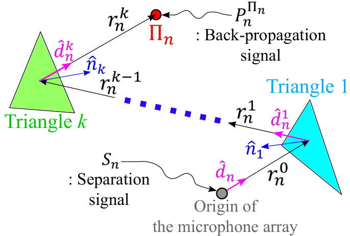
For the -th acoustic ray path, denoted by , its primary acoustic ray, , is created in to the -th direction vector , as shown in Fig. 4. If the acoustic ray collides with an obstacle, its secondary, reflection ray is generated by assuming the specular reflection, and is denoted by , where the superscript represents the order of the acoustic ray path. When is propagated until a -th order, the acoustic ray path consists of acoustic rays: i.e., .
IV-C Back-propagation signals
We introduce how to compute back-propagation signals based on acoustic ray paths and separation signals ; there is a tuple of for the direction vector that is the inverse direction of the -th incoming sound. We want to compute the back-propagation signal from the separation signal by designing and using an impulse response of backward sound propagation based on the acoustic ray path . The impulse response describes the reaction of any linear system as a function of time-independent variables; the input is the separation signal and the output is the back-propagation signal in our system.
In this work, we utilize the impulse response for the backward propagation to improve the accuracy of the sound source localization. In the forward sound propagation, the impulse response of an acoustic ray path is described by attenuations according to the travel distance of a ray path and reflection. For example, the travel distance attenuation represents the decrease of sound pressure inversely proportional to the travel distance of the ray path, because the sound is propagated according to the spherical wave in 3D environments; similar for the reflection attenuation.
On the other hand, for the backward propagation problem, the attenuation of travel distance and reflection becomes an amplification of the sound pressure. Suppose that we aim to compute the back-propagation signal from the starting point to a specific point (Fig. 4) on an acoustic ray path using the backward impulse response, where there is the -th tuple and the acoustic ray path consists of acoustic rays ; is a primary ray and is the -th reflection ray . In the frequency domain, the backward impulse response is described by amplifications because of the travel distance and the reflection until the -th order reflection ray :
| (3) |
where the term inside the exponential function is for shifting the back-propagation signal to the time delay of the sound propagation at the specific point and is the speed of sound. is a coefficient of the travel distance amplification, and is defined by a function of the travel distance : . Also, is a coefficient of the reflection amplification, and is defined by considering specular reflections until the -th order reflection ray:
| (4) |
where denotes the reflectivity (reflection coefficient) of the triangle hit by the -th order ray; the reflection coefficient is a function of frequency and we refer to coefficient values reported by [13].
The back-propagation signal at the specific point on the acoustic ray path is finally computed by the product of the backward impulse response and the separation signal in the frequency domain:
| (5) |
IV-D Estimating a source position
We now explain how to estimate the source position using back-propagation signals of acoustic ray paths.
The Monte Carlo sound source localization algorithm identifying the convergence region of acoustic ray paths was suggested in the prior work (RA-SSL) [2]; the convergence region means the area where acoustic ray paths gather. However, in real environments containing a moving source, obstacles, and noises, the accuracy of RA-SSL can decrease. For example, when there are background noises or complex configurations with obstacles, they can trigger to generate many arbitrary or incoherent acoustic ray paths, which may cause many convergence regions. If some cases, those convergence regions may be considered stronger than the one of the ground truth, deteriorating the accuracy of the localization method. By considering back-propagation signals, we aim to identify those arbitrary and incoherent acoustic ray paths and cull away acoustic ray paths with different back-propagation signals indicating that they are from different sound sources.
Intuitively speaking, if there are two acoustic ray paths caused by the same source, their back-propagation signals should be similar near the location of their sound source. In other words, when back-propagation signals of two acoustic ray paths are different at a location, the location is unlikely to be a candidate for a converging region of the sound source. Based on this observation, we design and utilize similarity between back-propagation signals for robustly identifying the sound source’s location even in these difficult settings.

Our estimation process is based on the Monte Carlo localization algorithm consisting of three parts: sampling, computing a weight of particles, and resampling. The main differentiation of our approach over the prior technique is that our method improves the localization accuracy based on a novel module for computing weights of particles based on our back-propagation signals.
Suppose there are -th particles, , representing hypothetical locations of the sound source at a frame. We would like to compute how close the particle is to acoustic ray paths. For this, we define a specific point , which is decided to be the point satisfying the shortest distance between and any point on the -th acoustic ray path; i.e., , where is the perpendicular foot on the -th acoustic ray path from the position (Fig. 5). We then compute our back-propagation signal according to Eq. 3 on the shortest point on the -th acoustic ray path from the particle .
From the back-propagation signal in the frequency domain, we compute the back-propagation signal in the time domain signal. We then calculate a particle weight, , representing the probability of being a convergence region of the sound source, based on two factors: a distance weight, , representing how away the particle is from the -th acoustic ray path and a similarity weight, , indicating how similar between and other signals given acoustic ray paths:
| (6) |
where is the number of acoustic ray paths at the frame, is the observation containing and , is a normalizing constant, and denotes a parameter for adjusting different weights.
The distance weight is calculated by using the Euclidean distance between the particle location and the point :
| (7) |
where is the Gaussian distribution function with the zero mean and a standard deviation . is maximized when the particle is on the perpendicular foot , which is on the -th acoustic ray path . The similarity weight measures the similarity between the back-propagation signal from the -th acoustic ray path and ones of other acoustic ray paths:
| (8) |
where is the normalizing constant, is the length of the back-propagation signal, is the peak coefficient in a normalized range of to , is the peak coefficient delay, and denotes the threshold value of . Both variables of and are computed by applying the cross-correlation operation between two signals, -th and -th signals:
| (9) | ||||
where is the cross-correlation operator.
As shown in Fig. 6, represents how much both back-propagation signals are correlated, and shows the time difference of occurrence between both back-propagation signals. As both back-propagation singles are from the same sound source, ideally and become one and zero, respectively.
Getting back to Eq. 8, we treat that two back-propagation signals are similar, when their peak coefficient is bigger than the threshold, i.e., . In this case, we assign a higher weight according to the relative time delay of the length of the signal, ; i.e., we give the highest weight when two signals are matched without any delay, under the assumption that those two signals are originated from the same sound source.

V RESULTS and DISCUSSION
In this section, we show how our approach accurately estimates the sound source location by measuring distance errors between the ground truth and the estimated position. The yellow disk in Fig. 1 represents a 95% confidence area for the estimated source. We also compare distance errors of our approach to the prior work (RA-SSL) to demonstrate the effectiveness of our algorithm considering the back-propagation signals; RA-SSL is the version of our approach without using the similarity of the back-propagation signals.
The hardware platform consists of Eigenmike, which is the 32-channel microphone array of the mh acoustics, and the i7 CPU computer. For reconstructing indoor environments, we first collect a point cloud by using Kinect v1 and then build a mesh map consisting of triangles from the point cloud; the reflection coefficients are appropriately assigned to the triangles by referring the reported values in [13].
We report values of parameters used for our algorithm: for controlling the influence of each weight is , the standard deviation of the Gaussian distribution function used for computing the distance weight is 0.5 that is determined by the consideration of the size of the indoor environment (about one tenth of the room width 7m), and the threshold value for checking the correlation between back-propagation signals is 0.15. We also show the results over different parameter values in Sec. V-C.
We use 3840 samples for the separation signal, where the sampling frequency is 48 kHz; 3840 audio samples (80 ms) are a sufficient length for covering direct and first reflection signals as indicated in [4].
V-A Benchmarks
Different experiments were conducted in two scenes: the moving sound without and with an obstacle. In both environments (Fig. 7a and Fig. 7b), a robot equipped with an omni-directional speaker moved along the red trajectory, and the 32-channel microphone array recorded the audio signals, and these data are used for various tests with the ground truth information on the sound source locations. In Fig. 7b, we put an obstacle made by paper boxes, to cause the robot invisible along the robot’s trajectory for the microphone array; at the invisible area, the sound source becomes the non-line-of-sight (NLOS) source.
Handling the NLOS source was reported to be a quite difficult problem in RA-SSL, because direct sound propagation paths are blocked by the obstacle and we have to rely on indirect sound paths that are incoherent and sensitive to noise. Furthermore, the number of indirect acoustic ray paths passing near the ground truth is usually small, and thus the accuracy of the localization algorithm tends to deteriorate.
Additionally, these scenes are not free from noise naturally occurring in a typical environment; they are exposed to noises, as shown in Fig. 9, since they are not controlled scenes. Noises can cause to trigger many incoherent acoustic ray paths, hindering them to converge in a single location.


V-B A moving sound source
We first show how our approach has the advantage compared to RA-SSL in a simple scene with a moving sound. In Fig. 8a, the black and red graphs denote the distance errors of RA-SSL and our approach, respectively. The average distance errors across the whole test time are 0.9231m for RA-SSL and 0.5594m for our approach; the accuracy of the sound source localization is improved about 65% based on our approach.
The experiment environments in Fig. 7 have many kinds of noises, caused by experimenters and the outside, as shown in Fig. 9, and these noises generate acoustic rays that do not help to localize the sound source. Especially, when the moving sound source turns the corner from 60 s to 70 s, the accuracy of RA-SSL deteriorates significantly. In this case, RA-SSL estimates source positions incorrectly near the noisy area (Fig. 9), while their signals from the noise source and from the ground truth source are different. On the other hand, the red graph shows that our method is robust even in this case, thank to considering the back-propagation signals on estimated source locations; the similarity weight improves the robustness of the source localization algorithm.
V-C A moving sound around an obstacle
We now show results with the more challenging environment including an obstacle between the source trajectory and the microphone array shown in Fig. 7b. Fig. 8b shows graphs of the distance errors of RA-SSL and our approach. The average distance errors of RA-SSL and our approach are 1.4919m and 0.4623m, respectively. Especially, where the sound source is in the NLOS state from 40 to 70 seconds, the accuracy of RA-SSL decreases drastically, because blocking the direct sound propagation paths makes the convergence of acoustic rays weak near the ground truth. On the other hand, even in this challenging case, we get a stable result, 220% improvement compared to RA-SSL, by considering similarity between back-propagation signals of indirect acoustic paths.
To analyze effects of varying values of , , and , we measure the average distance errors over various parameter values. Table I shows that our algorithm is robust to changes of parameters, where values of , , and vary from 0.5 to 1.5, from 0.3 to 0.7, and from 0.1 to 0.15, respectively. However, if the value of , the threshold for checking the peak coefficient, becomes 0.17, the accuracy dramatically decreases. This is mainly because coefficients of pairs of back-propagation signals originated by the same source have values from 0.17 to 0.23. As a result, when becomes too large, equal to or bigger than 0.17, we even filter out similar signals, and this enforces our approach to fall back to behave like the prior method RA-SSL. Nonetheless, our approach even in this case outperforms the prior method; RA-SSL’s average error is 1.4919m.
| 0.5 | 0.75 | 1.0 | 1.25 | 1.5 | |
| , | 0.55m | 0.52m | 0.46m | 0.63m | 0.6m |
| 0.3 | 0.4 | 0.5 | 0.6 | 0.7 | |
| , | 0.44m | 0.48m | 0.46m | 0.57m | 0.65m |
| 0.1 | 0.125 | 0.15 | 0.175 | 0.2 | |
| , | 0.52m | 0.47m | 0.46m | 1.12m | 1.3m |
V-D Analysis of back-propagation signals
Let us see how back-propagation signals have positive effects on the 3D sound source localization. Fig. 10 shows four separation signals observed from different incoming directions of the same sound source. On the right side of the figure, we also show four back-propagation signals generated from those observed separation signals at a location of the ground truth. The width of the red rectangle (a) shown on the left side of the figure indicates the time difference, caused by the distance difference of sound propagation paths, of separation signals. After computing the back-propagation signals from those separation signals, we observe that the time difference, denoted by the width of the red rectangle (b), of back-propagation signals was reduced. The reduction of the time difference in (b) compared to (a) can be interpreted that the back-propagation signals are restored better, since they are all originated from the same sound source.
We also measure cross-correlation between signals. When every pair of separation signals in Fig. 10 are analyzed by the cross-correlation operation, the average of peak coefficients and peak coefficient delays are 0.2183 and 280 samples, respectively. For the back-propagation signals, the average of peak coefficients and peak coefficient delays are 0.2245 and 35 samples. These values indicate that the computed back-propagation signals are restored in a way that those signals are similar to each other. Note that a higher peak coefficient indicates more correlated signals, and the peak coefficient delays close to zero represents that signals are well-aligned in time.
VI Limitations and Conclusion
We have presented a novel sound source localization algorithm using back-propagation signals. After estimating propagation paths of the sound by generating acoustic ray paths, the back-propagation signal virtually computed at a specific point on the acoustic ray path is considered. We utilize those back-propagation signals of different acoustic paths for robustly identifying the converging region of the source, even in environments with noises and an obstacle.
While we have demonstrated benefits of our approach, it has several limitations and opens up many interesting future directions. In Fig. 8, in some cases, our accuracy is lower than the prior work because of cropping a specific length of an audio signal from a measured signal at the microphone every fixed cycle; the cropped signal may not be able to collect enough audio signal at the beginning of the sound. We plan to deal with this problem by cropping and processing a meaningful audio signal from a measured signal at the microphone. Currently, real-time computation of our method is not ensured, due to the premature implementation of our current proof-of-concept system; the beamforming module runs in Matlab and the cross-correlation operation performed in pairs of available acoustic ray paths (e.g., 8 paths on average in our tests) runs serially. We plan to address this issue by re-implementing the beamforming module in C++ and designing the cross-correlation operations in a parallel manner.
Other sound propagation phenomena that are frequently observed at low frequencies or in the low frequency region such as scattering and diffraction are not handled yet. Fortunately, a ray tracing based approach supporting the diffraction effect is recently proposed [1], and can be adopted for our method. The acoustic material properties such as reflection coefficients of triangles of objects are not automatically assigned, and some of deep learning approaches showing promising results can be employed to solve this problem [13].
References
- An et al. [2018a] Inkyu An, Doheon Lee, Jung-woo Choi, Dinesh Manocha, and Sung-eui Yoon. Diffraction-aware sound localization for a non-line-of-sight source. arXiv preprint arXiv:1809.07524, 2018a.
- An et al. [2018b] Inkyu An, Myungbae Son, Dinesh Manocha, and Sung-eui Yoon. Reflection-aware sound source localization. In ICRA, 2018b.
- Cao et al. [2016] Chunxiao Cao, Zhong Ren, Carl Schissler, Dinesh Manocha, and Kun Zhou. Interactive sound propagation with bidirectional path tracing. ACM Transactions on Graphics (TOG), 35(6):180, 2016.
- Chen and Benesty [2011] Jingdong Chen and Jacob Benesty. A time-domain widely linear mvdr filter for binaural noise reduction. In Applications of Signal Processing to Audio and Acoustics (WASPAA), 2011 IEEE Workshop on, pages 105–108. IEEE, 2011.
- Khaykin and Rafaely [2009] Dima Khaykin and Boaz Rafaely. Coherent signals direction-of-arrival estimation using a spherical microphone array: Frequency smoothing approach. In Applications of Signal Processing to Audio and Acoustics, 2009. WASPAA’09. IEEE Workshop on, pages 221–224. IEEE, 2009.
- [6] C. Knapp and G. Carter. The generalized correlation method for estimation of time delay. IEEE Trans. Acoust., Speech, Signal Process., 24(4):320–327.
- Li et al. [2018] Dingzeyu Li, Timothy R Langlois, and Changxi Zheng. Scene-aware audio for 360° videos. arXiv preprint arXiv:1805.04792, 2018.
- Li et al. [2011] Xuan Li, Shefeng Yan, Xiaochuan Ma, and Chaohuan Hou. Spherical harmonics music versus conventional music. Applied Acoustics, 72(9):646–652, 2011.
- Rafaely [2005a] Boaz Rafaely. Analysis and design of spherical microphone arrays. IEEE Transactions on speech and audio processing, 13(1):135–143, 2005a.
- Rafaely [2005b] Boaz Rafaely. Phase-mode versus delay-and-sum spherical microphone array processing. IEEE signal processing Letters, 12(10):713–716, 2005b.
- Rafaely [2015] Boaz Rafaely. Fundamentals of spherical array processing, volume 8. Springer, 2015.
- Schissler et al. [2014] Carl Schissler, Ravish Mehra, and Dinesh Manocha. High-order diffraction and diffuse reflections for interactive sound propagation in large environments. ACM Transactions on Graphics (TOG), 33(4):39, 2014.
- Schissler et al. [2018] Carl Schissler, Christian Loftin, and Dinesh Manocha. Acoustic classification and optimization for multi-modal rendering of real-world scenes. IEEE transactions on visualization and computer graphics, 24(3):1246–1259, 2018.
- [14] J.-M. Valin, F. Michaud, and J. Rouat. Robust localization and tracking of simultaneous moving sound sources using beamforming and particle filtering. Robot. Auton. Syst., 55(3).
- Yan et al. [2011] Shefeng Yan, Haohai Sun, U Peter Svensson, Xiaochuan Ma, and Jens M Hovem. Optimal modal beamforming for spherical microphone arrays. IEEE Transactions on Audio, Speech, and Language Processing, 19(2):361–371, 2011.
- Yeh et al. [2013] Hengchin Yeh, Ravish Mehra, Zhimin Ren, Lakulish Antani, Dinesh Manocha, and Ming Lin. Wave-ray coupling for interactive sound propagation in large complex scenes. ACM Transactions on Graphics (TOG), 32(6):165, 2013.