Scaling and crossover behaviour in a truncated long range quantum walkJournal: Physica A

Discrete time quantum walks on discrete space have been studied extensively over the last couple of decades [1, 2, 3, 4]. In the quantum walk in one dimension, the state of the walker is expressed in the $|x\rangle\otimes|d\rangle$ basis, where $|x\rangle$ is the position (in real space) eigenstate and $|d\rangle$ is the chirality or coin eigenstate (either left ($|L\rangle$) or right ($|R\rangle$)). At each time step, there is a rotation and a translation operation on the walk which spreads according to the initial condition. The time dependence of the square of the displacement for a quantum walk is $\langle x^{2}\rangle\propto t^{2}$ showing it is much faster than the classical walk (where $\langle x^{2}\rangle\propto t$), and hence can play a key role in many dynamical processes.

Various studies have also been made by modifying the walk in suitable ways. In a large proportion of these works, the effect of disorder has been studied [5]. In some recent works, the disorder has been incorporated in the quantum walk in one dimension by considering long range step lengths chosen randomly at each discrete time step [6, 7]. Variable range step length in a discrete quantum walk along with memory effects was also studied in [8, 9].

With a binary choice of step lengths, the main result was the observation that there is a sub-ballistic but super-diffusive scaling for the second moment; $\langle x^{2}\rangle\propto t^{1.5}$ asymptotically [6]. In [7], Poissonian and other exponentially decaying distributions for the step lengths were used and a similar scaling was found (the exponent was reportedly $\sim 1.4$ obtained from a short time range). The scaling of the variance of $x$ is found to be parameter dependent for the non-Markovian walks considered in [8, 9], with a maximum value of the exponent equal to 3. In this context it may be mentioned that long ranged jumps were also considered albeit in a different manner, arising due to reasons like inhomogeneity of the material or geometry of the interferometer [10]. The scaling behaviour in this case was found to be completely different. However, as this long ranged walk does not belong to the class considered in [6, 7, 8, 9], it is not relevant for the present work and will not be discussed further. It may also be mentioned that when decoherence is induced by periodic measurements, the walk may be regarded as one with random step lengths [11]. However, this walk, characteristed by a time dependent periodicity, also belongs to a different class of problems and shows a ballistic to diffusive crossover.

In this paper, we choose the step lengths $\ell$ from a distribution

which is fat tailed. Moreover, we impose a cut-off in $\ell$ such that it is like a truncated Levy walk. Hence $A$, the normalization constant, is given by

Note that here the distribution is not truncated at a particular value as in [7], but rather, the maximum step length $\ell_{max}$ is kept fixed. Thus there are two independent parameters of this distribution, namely, $\delta$ and $\ell_{max}$. The case considered in [6] thus becomes a special case of the distribution (1) by putting $\ell_{max}=2$ and the probability $P(\ell=1)$ or $P(\ell=2)$ can then be expressed in terms of $\delta$. Here, we have used $\delta\geq 0$ in general which implies larger step lengths are less probable.

In quantum transport phenomena such Levy distributions have been considered in several earlier works. For the tight binding model which includes interaction with a thermal bath of oscillators [12], the effect of long range hopping has been studied. Also, continuous time quantum walks have been considered on discrete one dimensional lattices with long range steps (with a cut-off), where the interaction strength in the Hamiltonian decays as a power law with the step length [13]. In [14], both long range hoppings and long range interactions were incorporated for hard core bosons.

The quantum walker with disorder (QWWD henceforth) may be slower than the quantum walker without disorder (QWWOD henceforth) as already revealed in the earlier works, but because of the longer step lengths it can reach larger distances. Therefore one of the aims in studying the long ranged quantum walk is to find out its ability to search for remote targets. Another is to check its dependence on the nature of the distribution of the step lengths.

In this paper, we study the scaling behaviour of $\langle x\rangle$ and $\langle x^{2}\rangle$ for the fat tailed distribution given by Eq. (1). Next, we focus on the form of $f(x,t)$, the probability distribution that the walker is at site $x$ at time $t$. Lastly, we calculate the von Neumann entropy of entanglement which develops between the position and the coin states for the long ranged walks. Note that no measurement is being made at any time for this walk.

We generate the QWWD in the usual manner using a Hadamard coin. The process is exactly the same as described in [6] with $\ell$ chosen randomly at every step following Eq. (1). The state of the particle, $\psi({x},t)$, can be written as

The walk is initialized at the origin with $\psi_{R}(0,0)=a_{0},\psi_{L}(0,0)=b_{0};~~a_{0}^{2}+b_{0}^{2}=1$ and $\psi_{L}(x\neq 0,t=0)=\psi_{R}(x\neq 0,t=0)=0$. We choose $a_{0}=\sqrt{\frac{1}{3}}$ and $b_{0}=\sqrt{\frac{2}{3}}$ [15] such that in absence of disorder, an asymmetric probability density profile is obtained and one can study the scaling of both the first and second moments.

For any value of $\delta$, for a faithful representation of $P(\ell)$, one needs to generate a sufficient number of random step lengths. This poses a computational difficulty which increases with larger values of both $\delta$ and $\ell_{max}$. The number of step lengths generated is the maximum iteration time (i.e. the time up to which the walk is generated) multiplied by the number of configurations. One has to keep fixed the maximum time of iteration (to restrict the space spanned by the walker) and then for each value of $\ell_{max}$, the minimum number of configurations required for a faithful representation of the distribution is found out. This naturally determines also the maximum value of $\delta$ which can be used for a given value of $\ell_{max}$. Obviously, for larger $\ell_{max}$, we have to restrict to smaller values of $\delta$. This paper reports the cases for $4\leq\ell_{max}\leq 12$ and $0\leq\delta\leq 9.5$ (the maximum value of $\delta=9.5$ corresponding to $\ell_{max}=4$). The number of iterations is $t=10000$ used for $\ell_{max}=4$ and $t=3000$ for $\ell_{max}=12$. The number of configurations used is larger for larger values of $\ell_{max}$ for the reasons stated above; for example, it is 50000 for $\ell_{max}=12$ and 10000 for $\ell_{max}=4$.

The probability $f(x,t)$ for the particle to be at $x$ is given by $|\psi_{L}({x},t)|^{2}+|\psi_{R}({x},t)|^{2}$ and adds up to unity for all $t$. It has typically a central peak and two ballistic peaks occurring at nearly extreme values of $x\sim t$. We find that except for the region very close to the ballistic peaks, a data collapse can be obtained by plotting $f(x,t)t^{\gamma}$ against $x/t^{\gamma}$ with $\gamma=0.5$. Fig. 1 shows the results for the collapse of the centrally peaked region for $\ell_{max}=12$ and two extreme values of $\delta$.

The first two moments are evaluated as a function of time; the plots are shown in Fig. 2 for $\ell_{max}=12$ and $\delta=0$ and 5. Clearly, the asymptotic variation is $\langle x\rangle\propto t^{1/2}$ and $\langle x^{2}\rangle\propto t^{3/2}$. Following [6], we attempt to fit the moments using the equations

and

and find that a good consistency can be achieved. These equations had been arrived at using an approximate form of $f(x,t)$ assuming delta function like behaviour at $x=0$ and at the two extreme values of $x$ corresponding to the ballistic peaks. This approximation may not work well here as the collapse for the ballistic peaks is not as accurate as in [6] when one plots $f(x,t)t^{\gamma}$ against $x/t^{\gamma}$ with $\gamma=1$, especially for small values of $\delta$ (only the tips of the ballistic peaks, which have finite widths for small $\delta$, merge). This is borne by the fact that one obtains negative values of $b_{3}$ for small values of $\delta$ which is unphysical. Hence we do not proceed with further analysis of the parameters although the fitting is found to be good. It may also be added that scaling behaviour of the moments discussed above is independent of the value of $\ell_{max}$ and $\delta$.

Next we analyze in detail the characteristic features and form of the distribution $f(x,t)$. Note that in most of the earlier works, the disorder, usually incorporated through the coin operator, resulted in the transition to a Gaussian distribution. In contrast, in the present case, where the step lengths are chosen from a Levy distribution, the form of $f(x,t)$ as a function of the space variable $x$ is non-Gaussian in general. It is also obvious from Fig. 1 that the nature of the distribution changes appreciably as $\delta$ is changed. In the following, we investigate the form of the centrally peaked region that is obtained after suitable rescaling of the data. The scaled distribution is written as $g(z)=f(x,t)t^{1/2}$ and is studied as a function of $z=x/t^{1/2}$ for the largest value of $t$ ($t_{max}$) used in the generation of the walk. We have observed that up to values of $x=\alpha t^{1/2}_{max}$ the data can be fitted to a unique scaled function, where $\alpha$ is dependent on $\delta$ and $\ell_{max}$. We thus discuss the behaviour of $g(z)$ for $z<z_{max}=\alpha$. For small values of $z$, $g(z)$ shows a stretched exponential behaviour while we note that there is a distinct power law decay for larger values of $z$. Thus we conclude the following behaviour for the scaling function $g(z)$:

For values of $\delta$ greater than $\simeq 4$, $z^{*}$ coincides with $z_{max}$ such that the power law region is absent. In Fig. 3, the data for three different $\delta$ values are plotted along with the best fit stretched exponential curves for $\ell_{max}=12$. The function $z^{-2}$ is shown separately.

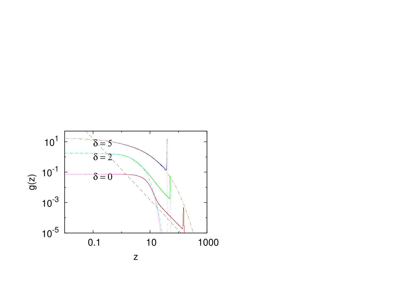
The values of $a,b,c$ are estimated for several values of $\ell_{max}$ and are shown as functions of $\delta$ in Fig. 4; all these quantities become independent of $\ell_{max}$ beyond $\delta\approx 4$.

The above results indicate that there exists a crossover behaviour for the scaling function $g(z)$ at $\delta=\delta^{*}\approx 4.0$, marked by two features. First, we find that the power law decay region of the scaling function $g(z)$ vanishes above this value of $\delta$. Secondly, beyond $\delta^{*}$, $g(z)$ becomes independent of $\ell_{max}$ ($\geq 4$) indicating universal behaviour beyond $\delta^{*}$ with respect to the cutoff.

In addition, we study two other quantities which depend on $\delta$ and also bear the signature of the crossover. The scaled distance $\langle x\rangle/\sqrt{t}$ travelled at time $t$ is found to be of the form

where the value of $\kappa$ is $\approx 2.55\pm 0.03$ for $\ell_{max}>4$ and $2.60\pm 0.01$ for $\ell_{max}=4$. The exponent value is obtained by fitting the data for $\delta\geq 0.5$. We conclude that $\kappa$ is a universal exponent $\approx 2.6$ independent of $\ell_{max}$ as the values differ by less than ten percent.

The range $R$ over which the probability distribution is nonzero ($>10^{-12}$ numerically) is also calculated. Since the ballistic peaks occur at values of $x\sim t$, the time up to which the walk is generated, $R$ is expected to scale as $t$. Hence $R$ is scaled by $t$ to find out whether any universal behaviour exists. It is found that $R/t$ has the form

The value of $r$ shows an approximate linear increase with $\ell_{max}$ while $s$ is very close to $\sqrt{2}$ independent of $\ell_{max}$. Note that for the QWWOD, the peaks occur at $x\approx t/\sqrt{2}$ such that the range at large times is approximately $\sqrt{2}t$ and the scaled range is $\sqrt{2}$ which coincides with the value obtained here for $\delta\to\infty$. The results for $\langle x\rangle/t^{1/2}$ and $R/t$ are also shown in Fig. 4.

Both $\langle x\rangle/t^{1/2}$ and $R/t$ derived from the probability distribution $f(x,t)$ show the signals of a crossover behaviour as expected. However, we find that the result for the QWWOD limit is attained only by $R/t$ as it saturates to the value $\sqrt{2}$ quite fast beyond $\delta^{*}$. This is due to the fact that the central hump, present even at large values of $\delta$, affects all other quantities but not the range.

The steep rise of $\langle x\rangle$ with $\delta$ can be understood qualitatively. It is noted that $f(x,t)$ becomes more asymmetric as $\delta$ is increased (note that for $\delta\to\infty$, when the model becomes effectively short ranged and deterministic, one has an asymmetric form for $f(x,t)$ with the chosen initial condition). This is clearly indicated by the numerical values of $\langle x\rangle$ which increase with $\delta$ according to Eq. (6). Even with $\delta$ as large as 9, $\langle x\rangle\simeq 816$ with $\ell_{max}=4$ while it is $\simeq 1786$ for the QWWOD. Apart from the fact that the asymmetry increases with $\delta$, another reason for $\langle x\rangle$ to increase with $\delta$ is that the height of the central peak decreases with $\delta$. Thus the contribution from larger values of $x$ become more significant in the expectation value of $x$, justifying the rather fast non linear increase of $\langle x\rangle$ with $\delta$.

Lastly, we investigate the so called quantumness of the process by looking at the entanglement measure for different values of the parameters. We calculate the von Neumann entropy of the reduced density matrix by taking trace over the position variables [16, 17, 18]. Note that the initial state is $|0\rangle\otimes(a_{0}|L\rangle+b_{0}|R\rangle)$ for which the von Neumann entropy is zero but the entanglement between the position and the coin space develops as the walk progresses. The entropy of the QWWOD is known to be dependent on the initial configuration. Since the asymptotic entanglement is already quite large for the QWWOD with the initial condition used, we show the results for another initial condition ($a_{0}=1,b_{0}=0$) for which the asymptotic value is less. It is seen that the entropy of entanglement for the QWWD, even at large values of $\delta$, are very close to 1, independent of the initial configuration, and as expected, larger than the QWWOD. On the other hand, we note that the oscillations are less in amplitude which indicates that the interference effects are less, consistent with the existence of the central hump occurring even for large (finite) values of $\delta$. We show in Fig. 5 the entropy of the long ranged walk in comparison to the QWWOD. As expected, we find that for $\delta=5$, which is larger than $\delta^{*}$, the results are independent of $\ell_{max}$ for both the initial conditions.

The present work had two aspects, first the effect of long range steps taken from a fat tailed distribution and second the truncation of the maximum step length. As obtained in the previous studies of random long ranged quantum walks [6, 7], one finds $\langle x^{2}\rangle\propto t^{3/2}$. This further strengthens the claim that the introduction of the long ranged steps modifies the scaling behaviour in a manner independent of the nature of the distribution $P(\ell)$.

It may be naively thought that for a choice of initial values of $a_{0}$ and $b_{0}$ which leads to a asymmetric form of $f(x,t)$, $\langle x\rangle$ will scale as $\sqrt{\langle x^{2}\rangle}\propto t^{3/4}$. However we find $\langle x\rangle$ behaves as $t^{1/2}$. One can justify this using the empirical analysis; $f(x,t)$ shows scaling behaviour with $x/t^{1/2}$ as the scaling variable (almost up to the point of the advent of the ballistic peaks) and since the contribution from the ballistic peaks nearly cancel out, the scaling behaviour is determined by the central region of $f(x,t)$ only.

The scaling function has been analyzed in some detail and it shows an interesting crossover behaviour. It may be recalled that the classical Levy walk shows a crossover to the short ranged behaviour (Gaussian form for probability distribution) beyond a certain value of the parameter $\delta$. Here, however, we do not get a crossover to the short ranged behaviour (which seems to be present only for $\delta\to\infty$ for $\ell_{max}>1$) but rather a change in the behaviour of the scaling function and also a universal behaviour with respect to $\ell_{max}$ for $\delta>\delta^{*}$. On the other hand the exponents are robust with respect to $\delta$, even for the largest value of $\delta$ considered. This may appear counter-intuitive as the system is expected to have short range behaviour for large values of $\delta$ but apparently, the peak at the center persists even for the maximum value of $\delta$ that could be simulated indicating that the interference effects are less effective compared to the QWWOD.

One may try to infer what happens if $\ell_{max}$ is made infinite, i.e., the unrestricted Levy walk. The present results indicate that above $\delta^{*}$, the scaling function has a stretched exponential behaviour that is independent of $\ell_{max}$. Hence it can be conjectured that the scaling function will have a stretched exponential behaviour for $\ell_{max}\to\infty$ as well for $\delta>\delta^{*}$. However, this needs more investigation since the results found here are all for finite values of $\ell_{max}$. One other interesting aspect of the long ranged walk is in the context of searching. We note that with $\delta<\delta^{*}$, the range is larger compared to that of the usual walker. So even though the walk is partially localised, it is possible to reach remote targets, the more so with larger $\ell_{max}$, albeit at a sub-ballistic speed.

When long term memory along with variable step lengths is considered, the variance shows a super-ballistic behaviour [8]. Hence from the present results, one can say it is the effect of memory that makes the walk faster and not the choice of time dependent step lengths.

One last point to be mentioned is the issue of quantumness. There have been some very recent works which suggest alternative ways of estimating this [19, 20] in quantum walks, these can be used in future studies.

Acknowledgement: The author acknowledges financial support from SERB project EMR/2016/005429. Discussions with Amit Kumar Pal and Suchetana Mukhopadhyaya are gratefully acknowledged.

References

- [1] Y. Aharonov, L. Davidovich, and N. Zagury, Phys. Rev. A 48, 1687 (1993).
- [2] J. Kempe, Contemp. Phys. 44, 307 (2003).
- [3] A. Nayak and A. Vishwanath, DIAMCS Technical Report 2000-43 and Los Alamos preprint archive, quant-ph/0010117.
- [4] A. Ambainis, E. Bach, A. Nayak, A. Vishwanath, and J. Watrous, Proceedings 33rd STOC New York (͑ACM, New York, 2001).
- [5] V. Kendon, Math. Struct. Comput. Sci. 17, 1169 (2007).
- [6] P. Sen, Physica A 514, 266 (2019).
- [7] S. Das, S. Mal, A. Sen(De), U. Sen, Phys. Rev. A 99, 042329 (2019).
- [8] G. Di Molfetta, D. O. Soares-Pinto and S. M. Duarte Queirós, Phys. Rev. A 97, 062112 (2018).
- [9] M. A. Pires, G. Di Molfetta, S. M. D. Queiros, arxiv:1907.12696 [quant-ph].
- [10] H. Lavic̆ka, V. Potoc̆ek, T. Kiss, et al. Eur. Phys. J. D 64, 119 (2011).
- [11] Y. Shikano, K. Chisaki, E. Segawa, and N. Konno, Phys. Rev. A 81, 062129 (2010); Y. Shikano, J. Horikawa and T. Wada, Phys. Scr. T151 014016 (2012) doi:10.1088/0031-8949/2012/T151/014016.
- [12] M. O. Cáceres and M. Nizama, J. Phys. A: Math. Theor. 43, 455306 (2010).
- [13] O Mülken, V. Pernice and A. Blumen, Phys. Rev. E 77, 021117 (2008).
- [14] T. Chattaraj and R. V. Krems, Phys. Rev. A 94, 023601 (2016).
- [15] Note that in [6], the same initial condition was taken but there is a typo in the published version. However, this is of no serious consequence.
- [16] Y. Ide, N. Konno and T. Machida, Quantum Information and Computation, 11 855 (2011).
- [17] G. Abal, R. Siri, A. Romanelli and R. Donangelo, Phys. Rev. A 73, 042302; 069905(E) (2006).
- [18] I. Carneiro, M. Loo, X. Xu, M. Girerd, V. Kendon and P. L. Knight, New J. Phys. 7, 156 (2004).
- [19] F. Shahbeigi, S. J. Akhtarshenas, A. T. Rezakhani, arXiv:1802.07027 [quant-ph]
- [20] V. Gualtieri, C. Benedetti, M. G. A. Paris, arXiv:1910.01563 [quant-ph]