Probing DAMA/LIBRA in the full parameter space of WIMP effective models of inelastic scattering
Abstract
We discuss the compatibility of the combined annual modulation effect measured by DAMA/LIBRA–phase1 and DAMA/LIBRA–phase2 with an explanation in terms of inelastic scattering events induced by the most general Galilean-invariant effective contact interaction of a Weakly Interacting Massive Particle (WIMP) dark matter particle of spin 0, 1/2 or 1. We take into account all the possible interferences among operators by studying the intersections among the ellipsoidal surfaces of constant signal of DAMA and other experiments in the space of the coupling constants of the effective theory. In our analysis we assume a standard Maxwellian velocity distribution in the Galaxy. We find that, compared to the elastic case, inelastic scattering partially relieves but does not eliminate the existing tension between the DAMA effect and the constraints from the null results of other experiments. Such tension is very large in all the parameter space with the exception of a small region for WIMP mass 10 GeV and mass splitting 20 keV, where it is partially, but not completely relieved. In such region the bounds from fluorine targets are evaded in a kinematic way because the minimal WIMP incoming speed required to trigger upscatters off fluorine exceeds the maximal WIMP velocity in the Galaxy, or is very close to it. As a consequence, we also find that the residual tension between DAMA and other results is considerably more sensitive on the astrophysical parameters compared to the elastic case. We find that the configurations with the smallest tension can produce enough yearly modulation in some of the DAMA bins in compliance with the constraints from other experiments, but the ensuing shape of the modulation spectrum is too steep compared to the measured one. For such configurations the recent COSINE–100 bound is evaded in a natural way due to their large expected modulation fractions.
pacs
95.35.+d,95.30.CqI Introduction
For more than 15 years the DAMA collaboration Bernabei et al. 2008a; Bernabei et al. 2010; Bernabei et al. 2013; Bernabei et al. 2018 has been measuring a yearly modulation effect in a large–mass low–background sodium iodide target compatible to the signal of the Dark Matter (DM) particles that are believed to make up 27% of the total mass density of the Universe Ade et al. 2014 and more than 90% of the halo of our Galaxy. Indeed, Weakly Interacting Massive Particles (WIMPs), which provide one of the most popular DM explanations, are expected to have feeble interactions with nuclear targets in a terrestrial detector with a scattering rate that presents a modulation with a period of one year due to the Earth revolution around the Sun Drukier et al. 1986. In particular, with the release of the latest DAMA/LIBRA-phase2 data Bernabei et al. 2018 the statistical significance of DAMA effect has reached almost . However, in the most popular WIMP scenarios used to explain the DAMA signal as due to WIMPs, the DAMA modulation appears incompatible with the results from many other DM experiments that have failed to observe any signal so far. Nevertheless, until recently none of the experiments ruling out the DAMA effect used the same target nuclei as DAMA/LIBRA, so that such incompatibility relied on both Particle–Physics and Astrophysics assumptions. Such model dependence has been shown to persist Kang et al. 2019 also after the bound from the COSINE–100 collaboration Adhikari et al. 2018a, that has recently published an exclusion plot for a standard elastic, spin–independent isoscalar WIMP nucleus interaction and a WIMP Maxwellian velocity distribution that for the first time rules out the DAMA effect at low WIMP masses using 106 kg of , the same target of DAMA. Given the strong statistical significance of the DAMA/LIBRA signal, and the scientific implications, this prompted the need to extend the class of WIMP models. Indeed, several scenarios have been introduced trying to reconcile the DAMA effect with other null results Kurylov and Kamionkowski 2004; Savage et al. 2004; Foot 2008; Feng et al. 2008; Bottino et al. 2008; Kouvaris 2008; Tucker-Smith and Weiner 2005; Savage et al. 2009a; Bai and Fox 2009; Savage et al. 2009b; Fox and Poppitz 2009; Feldstein et al. 2010; Kopp et al. 2010; Del Nobile et al. 2015; Kang et al. 2018a; Kang et al. 2019. A more systematic approach is to compare DAMA and other null results exploiting the non–relativistic (NR) nature of the WIMP–scattering process, that allows to express the interaction in terms of the more general effective Hamiltonian allowed by Galilean invariance Fitzpatrick et al. 2013; Anand et al. 2014, of the form:
| (1) |
where is the identity in isospin space, is the third Pauli matrix, and denotes the dark matter-nucleon relative distance and the operators depend on the exchanged momentum , the WIMP incoming velocity , the WIMP spin and nuclear spin . In Eq. (1) the isoscalar and isovector (dimension -2) coupling constants and , are related to those to protons and neutrons and by and . Truncating the effective theory expansion to operators at most quadratic in and the ensuing Hamiltonian contains 8 independent couplings for a scalar WIMP, 28 independent couplings for a spin–1/2 WIMP Fitzpatrick et al. 2013; Anand et al. 2014 and 20 couplings for spin–1 Dent et al. 2015. The ultimate assessment of the compatibility of DAMA with other constraints requires a full exploration of such large parameter space, where the relative sensitivities of different nuclear targets to DM scattering events may vary by orders of magnitude. While, due to the large dimensionality, its direct scanning appears to be challenging this has been achieved by using matricial techniques Catena et al. 2016, exploiting the fact that in terms of the couplings vector for all direct detection experiments the expected event rate can be written in the form:
| (2) |
with is a real symmetric matrix, which encodes all the information about nuclear responses, the dark matter velocity distribution, experimental efficiencies, etc., but which is independent of the underlying particle physics model (for a given dark matter mass). Due to this factorization in the effective field theory parameter space the surfaces of constant signal in different detectors are ellipsoids, and, as discussed in Refs. Catena et al. 2016; Catena et al. 2018, the determination of their geometrical intersections allows to efficiently compare the results of various direct detection experiments in the high-dimensional parameter space of the non-relativistic effective theory, without making any a priori assumptions regarding the relative size of the various Wilson coefficients . In this way for a standard halo model the DAMA/LIBRA–phase1 result Bernabei et al. 2008a; Bernabei et al. 2010; Bernabei et al. 2013 was shown to be incompatible to the constraints from other experiments in the case of elastic interactions of a WIMP particle with spin 1/2 and the interaction Hamiltonian of Eq.( 1) with arbitrary couplings combinations Catena et al. 2016.
As pointed out by the authors, the analysis in Catena et al. 2016 did not cover several alternative scenarios. One of them is inelastic scattering. Indeed, one of the very few scenarios that reconcile DAMA with the constraints of other experiments is proton–philic Spin–dependent Inelastic Dark Matter (pSIDM) Scopel and Yoon 2016; Scopel and Yu 2017; Kang et al. 2019. In such model the WIMP particle interacts with nuclear targets through a spin–dependent coupling that is suppressed on neutrons, in order to comply to constraints using neutron–odd scattering targets (germanium and xenon). Moreover inelastic scattering (IDM) Tucker-Smith and Weiner 2001; Chang et al. 2009; March-Russell et al. 2009 reconciles the above scenario to fluorine detectors. In IDM a DM particle of mass interacts with atomic nuclei exclusively by up–scattering to a second heavier state with mass . A peculiar feature of IDM is that there is a minimal WIMP incoming speed in the lab frame matching the kinematic threshold for inelastic upscatters and given by:
| (3) |
with the WIMP–nucleus reduced mass. This quantity corresponds to the lower bound of the minimal velocity (also defined in the lab frame) required to deposit a given recoil energy in the detector:
| (4) |
with the nuclear mass.
In particular, indicating with and the values of for sodium and fluorine, and with the WIMP escape velocity, in Refs. Scopel and Yoon 2016; Scopel and Yu 2017; Kang et al. 2019 constraints from WIMP–fluorine scattering events in droplet detectors and bubble chambers were shown to be evaded when the WIMP mass and the mass gap are chosen in such a way that the hierarchy:
| (5) |
is achieved. In fact, in such case WIMP scatterings off fluorine turn kinematically forbidden while those off sodium can still serve as an explanation to the DAMA effect. So the pSIDM mechanism rests on the trivial observation that the velocity for fluorine is larger than that for sodium.
In the present paper we wish to apply the technique introduced in Ref. Catena et al. 2016 to extend the analyses of Scopel and Yoon 2016; Scopel and Yu 2017; Kang et al. 2019 to the general interaction Hamiltonian of Eq. (1), or, conversely, we wish to extend the analysis of Catena et al. 2016 to the case of inelastic scattering, updating it to the present experimental situation and including the DAMA/LIBRA–phase2 data release and the state of the art of all the constraints from other experiments.
The two most important improvements of DAMA/LIBRA-phase2 compared to the previous phases are that now the exposure has almost doubled and the energy threshold has been lowered from 2 keV electron-equivalent (keVee) to 1 keVee. In particular this latter feature introduces an important difference between the present analysis and that of Ref. Catena et al. 2016. In the latter, for kinematic reasons and irrespective of the effective interaction the DAMA/LIBRA-phase1 data were only sensitive to scattering events off Sodium for a WIMP mass 20 GeV, implying that in such range of mass the scaling law induced by the effective Hamiltonian (1) only entered in the comparison of the scattering rate off Sodium and that off the targets of other experiments. However, due to the lower threshold, now for 20 GeV DAMA/LIBRA–phase2 is sensitive to both the target nuclei, with WIMP–Iodine scattering events contributing to the expected rate in the new low–energy range below 2 keVee and Sodium at higher energy. This implies that the scaling law among different targets is now also relevant in explaining the energetic spectrum of the modulation amplitudes measured by DAMA alone. Indeed, due to this reason for a standard Maxellian velocity distribution the the goodness–of–fit of a WIMP explanation of the DAMA/LIBRA-phase2 data has already been showed to worsen compared to DAMA/LIBRA-phase1 for a standard Spin-Independent interaction (SI) dam 2018; Baum et al. 2018, requiring to tune the ratio between the WIMP–proton and the WIMP–neutron couplings in order to suppress WIMP–Iodine scattering events below 2 keVee. As shown in Kang et al. 2018b, with the exception of and , which in the notation of Fitzpatrick et al. 2013; Anand et al. 2014 correspond respectively to the standard SI or Spin–Dependent (SD) interactions, this problem is not present for all the other operators of the Hamiltonian (Eq. 1). This represents an additional motivation to update the result of Ref. Catena et al. 2016 to the DAMA/LIBRA-phase2 data. Finally, the recent COSINE–100 bound is potentially relevant to our analysis because any probe of the DAMA effect using is expected to lead to conclusions independent on the WIMP–nucleus cross section scaling law and so on the particular choice of the couplings of the Hamiltonian (Eq. 1). However, as we will show, an important dependence on the Hamiltonian (Eq. 1) is still present when comparing COSINE-100 and DAMA. This is due to the fact that, although an initial modulation analysis of COSINE-100 with two–year data is forthcoming and an additional low–threshold analysis is also actively under development, COSINE-100 needs to collect several years of data Thompson 2017 in order to reach the sensitivity required to probe the DAMA signal, and until then COSINE–100 will only exploit the average count rate. So the results of the two experiments are presently based on two different observables, the yearly modulation expected from the rotation of the Earth around the Sun and the time–averaged rate, and their relative size does depend on the specific model of WIMP–nucleus interaction besides a standard SI or SD interaction with nuclei.
The paper is organized as follows: in Section II we summarize how we calculate WIMP direct detection rates in NR effective theory; in Section III we outline the geometrical method of Ref. Catena et al. 2016 that we use to study the intersections among the ellipsoidal surfaces of constant signal of DAMA and other experiments in the space of the coupling constants of the effective theory; our quantitative analysis is contained in Section IV. We devote Section V to our conclusions. For completeness we summarize the response functions of a WIMP of spin 1 in Appendix A and we provide the details of our treatment of experimental constraints in Appendix B.
II WIMP inelastic scattering in non-relativistic effective models
In the present Section we briefly summarize the ingredients that we use to calculate for each experiment and for each energy bin used in our analysis the matrix introduced in Eq. (2), needed to evaluate the expected rate to compare to the experimental data.
The full list of operators entering the Hamiltonian of Eq. 1 for the nuclear scattering process of a WIMP particle of spin 1 is given by:
| (6) |
In the equation above is the identity operator, is the transferred momentum, and are the WIMP and nucleon spins, respectively, while is the symmetric combination of polarization vectors in the case of a spin–1 DM particle and (with the WIMP–nucleon reduced mass) is the relative transverse velocity operator satisfying . For a nuclear target the quantity can also be written as Barello et al. 2014:
| (7) |
where is given by Eq.(4).
Operator is of higher order in compared to all the others, implying a cross section suppression of order for the non–relativistic WIMPs in the halo of our Galaxy. Moreover it cannot be obtained from the leading-order non relativistic reduction of a manifestly relativistic operator Fitzpatrick et al. 2013. So, following Refs.Fitzpatrick et al. 2013; Anand et al. 2014, we will not include it in our analysis. Moreover, operator is a linear combination of other operators, so can be omitted. This implies a maximal number of 16 operators in the effective Hamiltonian in Eq. (1), namely 4 operators for a spin–0 DM particle, 14 operators for spin 1/2 and 10 operators for spin 1.
To reduce the parameter space of the effective interaction of Eq. (1) in the following we will make a few simplifying assumptions. First, we will only consider the case 0, i.e. upscatters of a light state to a heavier one; then we will assume a contact effective interaction between the WIMP and the nucleus, i.e., we will assume the coefficients as independent on the transferred momentum and neglect propagator effects. Moreover, we will consider real ’s, although in general for an inelastic process they can be complex Barello et al. 2014. Finally, we will not consider the possibility of inelastic scattering among states of different spins Barello et al. 2014.
The expected rate in a given visible energy bin of a direct detection experiment is given by:
| (8) | |||||
| (9) | |||||
| (10) |
with the experimental efficiency/acceptance. In the equations above is the recoil energy deposited in the scattering process (indicated in keVnr), while (indicated in keVee) is the fraction of that goes into the experimentally detected process (ionization, scintillation, heat) and is the quenching factor, is the probability that the visible energy is detected when a WIMP has scattered off an isotope in the detector target with recoil energy , is the fiducial mass of the detector and T the live–time of the data taking. For a given recoil energy imparted to the target the differential rate for the WIMP–nucleus scattering process is given by:
| (11) |
where is the local WIMP mass density in the neighborhood of the Sun, the number of the nuclear targets of species in the detector (the sum over applies in the case of more than one nuclear isotope), while
| (12) |
with the nuclear target mass and, assuming that the nuclear interaction is the sum of the interactions of the WIMPs with the individual nucleons in the nucleus:
| (13) |
In the above expression and are the WIMP and the target nucleus spins, respectively, while the ’s are WIMP response functions (that we report for completeness in Eq.(29)) which depend on the couplings as well as the transferred momentum and . In equation (13) the ’s are nuclear response functions and the index represents different effective nuclear operators, which, crucially, under the assumption that the nuclear ground state is an approximate eigenstate of and , can be at most eight: following the notation in Fitzpatrick et al. 2013; Anand et al. 2014, =, , , , , , , . The ’s are function of , where is the size of the nucleus. For the target nuclei used in most direct detection experiments the functions , calculated using nuclear shell models, have been provided in Refs. Anand et al. 2014; Catena and Schwabe 2015 under the assumption that the dark matter particle couples to the nucleus through local one–body interactions with the nucleons. In our analysis we do not include two–body effects two 2013; two 2015 which are only available for a few isotopes and can be important when the one–body contribution is suppressed. Finally, is the WIMP velocity distribution, for which we assume a standard isotropic Maxwellian at rest in the Galactic rest frame truncated at the escape velocity , and boosted to the Lab frame by the velocity of the Earth. So for the former we assume:
| (14) | |||||
| (15) |
with . In the isothermal sphere model hydrothermal equilibrium between the WIMP gas pressure and gravity is assumed, leading to = with the galactic rotational velocity.
With the exception of DAMA, all the experiments included in our analysis are sensitive to the time average of the expected rate for which = and =+12 km/sec (accounting for a peculiar component of the solar system with respect to the galactic rotation). In the case of DAMA, the yearly modulation effect is due to the time dependence of the Earth’s speed with respect to the Galactic frame, given by:
| (16) |
where 0.49 accounts for the inclination of the ecliptic plane with respect to the Galactic plane, =1 year and =2 29 km/sec (=1 AU neglecting the small eccentricity of the Earth’s orbit around the Sun).
In our analysis for the two parameters and we take =220 km/sec Koposov et al. 2010 and =550 km/sec Piffl et al. 2014 as reference values, although in Section IV we will also discuss the dependence of the results when the same parameters are varied in the ranges =(220 20) km/s Koposov et al. 2010 and =(550 30) km/s Piffl et al. 2014. Our reference choice of parameters corresponds to the WIMP escape velocity in the lab rest frame 782 km/s. To make contact with other analyses, for the dark matter density in the neighborhood of the Sun we use =0.3 GeV/cm3, which is a standard value commonly adopted by experimental collaborations, although observations point to the slightly higher value =0.43 GeV/cm3 Salucci et al. 2010; Nesti and Salucci 2013. Notice that direct detection experiments are only sensitive to the product , so the results of the next Section can be easily rescaled with .
In particular, in each visible energy bin DAMA is sensitive to the yearly modulation amplitude , defined as the cosine transform of :
| (17) |
with =1 year and =2nd June, while other experiments put upper bounds on the time average :
| (18) |
Using the ingredients listed above, for a given value of the two parameters and both and can be expressed as quadratic forms like Eq. (2), i.e. for each of the experimental observable considered in our analysis a real symmetric matrix can be obtained. Schematically, for each energy bin and both for DAMA and for each of the other experiments :
| (19) | |||||
| (20) |
III Maximal DAMA signals compatible to null results
Following the analysis in Catena et al. 2016, in this section we will use the property that, for a fixed value of the WIMP mass and of the mass splitting , constant–rate surfaces in the couplings vector space are ellipsoids. In particular, given the experimental upper bound for experiment and energy bin , the condition implies that allowed configurations must lie inside the ellipsoid:
| (21) |
As far as the DAMA modulation amplitudes are concerned, the experimentally observed intervals in energy bins imply the additional upper bounds:
| (22) |
which add to the previous constraints. From now on we will indicate all upper bound matrices as , for , with the full set of experimental upper constraints including the upper bounds on the DAMA modulation amplitudes, so that the following conditions must be verified:
| (23) |
In our analysis we will include the 8 DAMA modulation amplitudes for 1 keVee 5 keVee Bernabei et al. 2018, and selected energy bins from XENON1T Aprile et al. 2018a, PICO–60 ( target) Amole et al. 2017; Amole et al. 2019, COSINE–100 Adhikari et al. 2018a, COUPP Behnke et al. 2012, SuperCDMS Agnese et al. 2018a and PICASSO Behnke et al. 2017. The details of how we implemented the DAMA effect and the bounds are provided in Appendix B and in Table 3. Given the DAMA modulation amplitudes, an explanation of the effect in terms of WIMPs implies also the lower bounds:
| (24) |
Compatibility between DAMA and the other experiments is achieved only if in the coupling constants parameter space the intersection between the volumes outside the ellipsoids =1, and the volume inside the ellipsoids =1, is non–vanishing. To prove this it is sufficient to find a set of real parameters that, for each DAMA energy bin satisfy Pólik and Terlaky 2007:
| (25) |
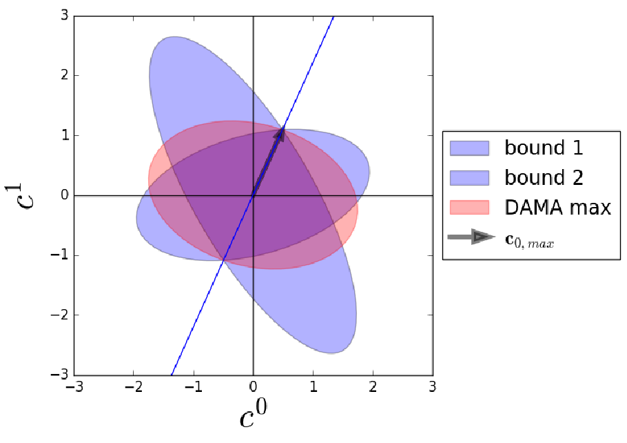
In particular, if the binary test above is verified no set of couplings exists for which the two conditions (23) and (24) are satisfied at the same time. Geometrically, this implies that the volume of intersection among the ellipsoids is fully contained in the DAMA ellipsoid of . On the other hand, when the matrix of Eq. (25) is not positive–defined such set of couplings exists. Notice that, in such case, since the matrices include the upper bounds on the DAMA modulation amplitudes, for that choice of the condition is automatically satisfied in the energy bin in compliance to all other existing constraints, although this is not guaranteed for the modulation amplitudes in the other energy bins. An alternative way to show the result of the test above is to calculate the maximal value of the modulation amplitude allowed by present constraints, i.e. to take in as a free parameter and find the minimal value for which the condition (25) is verified Catena et al. 2016; Catena et al. 2018. A schematic view of the intersection between the ellipse and the edge of the experimentally allowed volume in the coupling constants space is provided in Fig. 1 for the case of a single coupling and two upper bounds. Such value can then be converted in a number of standard deviations away from the measurement (in absolute value). The tension between DAMA and the other experiments can then be quantified as the maximum of among the DAMA energy bins calculated in the following way: i) we fix one target energy bin ; ii) we maximize the modulation signal in ; iii) for the corresponding set of couplings we calculate the modulation signal also in the other bins; iv) we take as the maximum tension among all the bins; v) we loop over the target bin and take the minimum (since each target bin yields a different model). Notice that the procedure described above may not yield the model which better reproduces the data in the bins where the maximal allowed modulation exceeds the central value of the measurement.
In total, we have solved Eq. (25) using 27 matrices (8+8 DAMA matrices plus 11 matrices for null results).
IV Analysis
In this section we discuss the parameter solving Eq. (25) using PICOS pic, a Python interface to conic optimization, together with the CVXOPT solver cvx.

The main results of our analysis is shown in Fig. 2. In such figure, for different value of the WIMP spin , the upper band shows as a function of in the elastic case (=0), while the lower bands represent minimized in terms of at fixed . The bands indicate the variation of when the parameters and of the Maxwellian distribution of Eq. (15) are varied in the ranges =(220 20) km/s Koposov et al. 2010 and =(550 30) km/s Piffl et al. 2014, while the solid line indicates the result for the reference values =220 km/s and =550 km/s. The gray shaded regions represent =0, the red bands =1/2 and the purple ones represent =1. As far as the =0 case is concerned, a DAMA explanation is excluded at more than 7 sigmas for all WIMP masses below 200 GeV. Compared to the elastic case, inelastic scattering partially relieves this tension with values as low as 4.0 for =0, 2.9 for =1/2 and 3.2 for =1. However is considerably more sensitive on the astrophysical parameters and compared to the elastic case. From this figure one can conclude that neither the large range of different interactions provided by the effective field theory nor the modified kinematics due to inelasticity can eliminate completely the tension between DAMA and experimental constraints.


When the quantity is plotted in the – plane a general result common to all values is that the region of parameter space where the tension is relieved is localized in a narrow region with 20 keV. In Figs. 3,4 and 5 we provide contour plots of centered on such localized regions of the – parameter space for =0, 1/2, 1, respectively, and for the three combinations (,)=(220,550),(200,520),(240,580) km/s. In all the plots the dotted (red) line represents the maximal value of beyond which the minimal speed introduced in Eq. (3) exceeds the escape velocity in the Lab frame, , while the (blue) short dashes show the minimal value of beyond which . This implies that between the two lines the condition of Eq. (5) is verified. The closed contour where the tension drops tracks for different astrophysical parameters the region between the two lines, an unequivocal indication that the same kinematic mechanism is at work as in the pSIDM scenario Scopel and Yoon 2016; Scopel and Yu 2017; Kang et al. 2019 summarized in the Introduction. This also explains why, as observed in Fig. 2, is considerably more sensitive on the astrophysical parameters and compared to the elastic case. So we conclude that the pSIDM scenario described in (Scopel and Yoon 2016; Scopel and Yu 2017; Kang et al. 2019) emerges as the unique mechanism to ease the tension between DAMA and other constraints from a general scan of the inelastic DM parameter space.
In spite of the residual tension between DAMA and other constraints it is interesting to discuss in detail the solutions corresponding to the minimum values of . In order to do so one needs to go back to Eq. (25). At the boundary of its positivity the smallest eigenvalue of the matrix in that equation is vanishing and the corresponding eigenvector (=1):
| (26) |
individuates the line joining the origin to the points of intersections between the extreme DAMA ellipsoid and those of the constraints, as shown schematically by the solid line in Fig. 1. On the other hand, the vector , joining the origin to the intersection points and given by:
| (27) |
contains the set of couplings for the configuration of maximal modulation amplitude in the bin , and in Fig. 1 is represented by the black arrow. The properties of the specific point in the space of couplings can be further elucidated if one takes a closer look at the matrices in Eqs. (19,20). Depending on the spin of the WIMP particle they can have a different dimensionality, as can be simply read–off from the WIMP response functions in Eqs. (29,30). Moreover, not all couplings interfere, so that the matrices can be decomposed into block-diagonal form. The dimensionalities and non–interfering subspaces are indicated in Table 1 for different values of the WIMP spin . This implies that also the matrix is block–diagonal, so that must belong to one of the subspaces of Table 1.
| spin | couplings | dimensionality |
|---|---|---|
| 0 | ,, | 2=8 |
| ,, | 2 | |
| , , , | =28 | |
| ,, | ||
| 1 | ,, , | 2 |
| , , , , | =20 |
| spin | (GeV) | (cm2) | |||
| 0 | 11.08 | 22.83 | 3.93 | (=0.68, =0.73) | 4.0 |
| 1/2 | 11.64 | 23.74 | 4.68 | (=-0.0014, =-0.0015, | 2.9 |
| =-0.032, =-0.0166, | |||||
| =0.692, =0.7217) | |||||
| 1 | 11.36 | 23.43 | 5.71 | (=0.0717, =0.0753, | 3.2 |
| =0.1892, =0.9764) |
The properties of the extreme configurations found in this way are given in Table 2. Interestingly, the configuration with the smallest tensions corresponds to a coupling for =0 (a spin–dependent interaction with explicit velocity dependence and momentum suppression )) and to approximately a coupling for =1/2 (a spin–dependent interaction with momentum suppression ). These two couplings combinations correspond to two of the possible generalizations of the pSIDM scenario already discussed in Scopel and Yu 2017. On the other hand, for =1 the extreme configuration corresponds to a dominant coupling (associated to the WIMP coupling to the orbital angular momentum operator) also with momentum suppression , and a non–negligible contribution. The role of momentum suppression in relieving the tension between the DAMA result and other constraints has already been pointed out in Scopel et al. 2015.
Our procedure does not correspond to the minimization of a –square, since we minimize the tension in one target bin at a time. However, once a minimal tension configuration is obtained, the quantity = (with and the measured modulation amplitudes and standard deviations) can be calculated. In this way, for the configurations of Table 2 we get =60.6, 25.7 and 33.5 for =0,1/2 and 1, respectively.


The corresponding predictions for the DAMA modulation amplitudes are shown in Figs. 6,7 and 8 for the different values of and compared to the measured ones Bernabei et al. 2018. In such figures the experimental points marked with a (red) circle correspond to the energy bins included in the solution of Eq. (25), while the point marked with an additional (blue) inner circle corresponds to the DAMA energy bin where the maximal tension with the bounds arises and that drives the determination of . As one can see in the lower energy bins the allowed modulation signal is large enough to explain the DAMA signal, although the amplitudes spectrum decays faster with energy.


Introducing the vector with a free normalization, is common to all signals inside the eigenspace of . A convenient parameterization is through the introduction of the reference cross section:
| (28) |
with the WIMP–nucleon reduced mass. The direction in coupling space singled out by the unit vector , and that individuates a specific set of coupling ratios that eases the tension between DAMA and the constraints, can be seen as the generalization in an arbitrary number of dimensions of the concept of isospin–violating DM Feng et al. 2011. Once and are fixed the DAMA signal and the bounds can be discussed in a familiar – plane. This is done in Figs. 9, 10 and 11 for the extreme configurations summarized in Table 2 and for =1, 1/2 and 1, respectively. In the same figure the (red) circle represents the point with the value of the WIMP mass for the extreme configuration and , . The point intersects one or more of the most constraining boundaries on at =, providing a nice confirmation of the numerical solution of Eq. (25). Actually, this can be directly observed in Figs. 9, 10 and 11 for for =0, 1/2 and 1, respectively, where the point lies on the intersection between the bounds from XENON1T and PICO–60, in a realization of the mechanism shown schematically in Fig. 1. In all three cases, the extreme configuration hits also the 90% C.L. upper bound on the modulation fraction in the first bin, as shown in Figs. 6, 7 and 8. In Figs. 9, 10 and 11 the distance from the DAMA region and the extreme point provides an additional visual indicator besides of the tension between DAMA and the constraints from null results. Indeed, as already observed in Kang et al. 2019, the condition (5) implies that inside the energy range of the DAMA effect the spectrum of the predicted modulation amplitudes has a maximum corresponding to the recoil energy = for scattering events off sodium. On the other hand, the data from DAMA/LIBRA-phase2 are more compatible to a monotonically decreasing shape11 1 The DAMA/LIBRA-phase1 data showed instead a maximum, and for this reason inelastic scattering could provide a good fit to the data Scopel and Yoon 2016. closer to elastic scattering. As a consequence, the DAMA data pull to low values of . However, the solutions of Eq. (25) with smallest tension with the constraints require sizeable values of ( 20keV) in order to verify Eq. (5). As a consequence, when is fixed to such values the DAMA data pull to higher values of the WIMP mass to dilute the effect of . This explains why, systematically, the DAMA regions in Figs. 9, 10 and 11 are at higher WIMP masses compared to the values of in Table 2. Moreover, Figs. 6, 7 and 8 show that configurations allowed by constraints from null results can produce enough yearly modulation in some of the DAMA bins, but the ensuing shape of the modulation spectrum is too steep, so that the maximal modulation at high energy is constrained by the bins at low energy. In light of this observation, we interpret the fact that all the smallest tension configurations of Table 2 have an interaction with explicit momentum suppression as a way to alleviate this problem by suppressing the DAMA modulation amplitudes in the lowest–energy bins.
These findings are in agreements to those of Ref. Kang et al. 2019, obtained for the specific case of a standard spin–dependent interaction.
Equation (25) can only be solved for a limited selection of experimental bounds both because of computing time limits, and because some of the constraints require more refined treatments beside a simple comparison between theoretical predictions and upper bounds as in Eq. (23) and Table 3, such as background subtraction or the optimal-interval method Yellin 2002. In Figs. 9, 10 and 11 all this standard machinery Kang et al. 2018c can instead be applied to the full set of existing experiments, providing an a posteriori confirmation that the set of bounds used to solve Eq. (25) did not miss any relevant constraint. In particular, besides the experiments included in the solution of Eq. (25), in such figures we have added CDMSlite Agnese et al. 2018b, CRESST-II Angloher et al. 2016; Angloher et al. 2017a, the upper bound from the average count rate of DAMA Bernabei et al. 2008b), DarkSide–50 Agnes et al. 2018 and the target run of PICO–60 Amole et al. 2015 (the details of such bounds implementation are provided in Appendix B). None of these additional null results further constrains the extreme configurations ().
We conclude by noting that the recent bound from COSINE–100 Adhikari et al. 2018a, obtained with the same target material as DAMA, is not particularly binding in our analysis, as can be seen again in Figs. 9, 10 and 11. The reason of this is that the bound of Ref. Adhikari et al. 2018a is on the time–averaged signal , while DAMA measures the yearly modulation amplitudes expected from the rotation of the Earth around the Sun . In appendix B we estimate in COSINE–100 a residual count rate 0.13 events/kg/day/keV after background subtraction while modulation fractions in DAMA are of the order of 0.02 events/kg/day/keV. The bound implies = 0.12, including a factor 0.8 due to a difference between the energy resolutions and efficiencies in the two experiments. For a standard Maxwellian WIMP velocity distribution in the SI elastic case the predicted modulation fractions are below such bound (for instance, for =10 GeV is between 0.05 and 0.12 for 3 keVee) explaining why in Ref. Adhikari et al. 2018a the DAMA effect is ruled out. However expected rates for inelastic scattering are sensitive to the high–speed tail of the WIMP velocity distribution for which the modulation fractions are sizeably higher Tucker-Smith and Weiner 2001; Scopel and Yoon 2016, and this is particularly true when the condition (5) is verified (for instance, in the extreme configurations of Table 2 we find 0.8 for 3.5 keVee).
V Conclusions
In the present paper we have discussed the compatibility of the combined annual modulation effect measured by DAMA/LIBRA–phase1 and DAMA/LIBRA–phase2 Bernabei et al. 2008a; Bernabei et al. 2010; Bernabei et al. 2013; Bernabei et al. 2018 with an explanation in terms of inelastic scattering events induced by the most general Galilean-invariant effective contact interaction of a spin 0, 1/2 or 1 WIMP dark matter particle taking into account all the possible interferences among operators by studying the intersections among the ellipsoidal surfaces of constant signal of DAMA and other experiments in the space of the coupling constants of the effective theory, following the approach introduced in Ref. Catena et al. 2016. In our analysis we have assumed a standard Maxwellian velocity distribution in the Galaxy. Compared to the elastic case, inelastic scattering partially relieves but does not eliminate the existing tension between the DAMA effect and the constraints from the null results of other experiments. We have determined the ellipsoids using 90% C.L. upper bounds from selected energy bins from XENON1T Aprile et al. 2018a, PICO–60 ( target) Amole et al. 2017; Amole et al. 2019, COSINE–100Adhikari et al. 2018a, COUPP Behnke et al. 2012, SuperCDMS Agnese et al. 2018a and PICASSO Behnke et al. 2017. The tension, quantified as the maximum of among the DAMA energy bins below 5 keVee, exceeds 7 in all the parameter space 200 GeV with the exception of a small region of parameter space for 10 GeV and 20, where it drops to values as low as 4 for =0, 2.9 for =1/2 and 3.2 for =1, and that overlaps to the proton–philic spin–dependent inelastic Dark Matter (pSIDM) scenario Scopel and Yoon 2016; Scopel and Yu 2017; Kang et al. 2019 already discussed in the literature for the specific case of a standard spin–dependent interaction, where the bounds from fluorine targets are evaded in a kinematic way because the minimal WIMP incoming speed required to trigger upscatters off fluorine exceeds the maximal WIMP velocity in the Galaxy, or is very close to it. In particular, from a general scan of the inelastic DM parameter space such kinematic feature, together with momentum suppression in the effective operator, emerge as instrumental in easing the tension between DAMA and other constraints. As a consequence, the latter is considerably more sensitive on the astrophysical parameters compared to the elastic case. The configurations for which the tension is partially relieved can easily produce enough yearly modulation in the lowest–energy bins of the modulation spectrum measured by DAMA in compliance with the constraints from other experiments. However, the ensuing shape of the modulation spectrum is too steep, so that, when not excluded by other constraints, the maximal allowed modulation at higher energies is constrained by the modulation measured in the lowest energy bins.
The present analysis extends the scope of previous ones in the task to explore a DAMA explanation in the full WIMP direct detection parameter space, but is still not the most general one. Possible extensions include: i) long–range interactions; ii) allowing for complex couplings; iii) assuming a WIMP velocity distribution that departs from a standard Maxwellian. In particular, given the large dependence on the astrophysical parameters that we observed in our results we expect the latter generalization as very promising in order to find effective models that reconcile the DAMA result with the null observations of other experiments.
Acknowledgements.
This research was supported by the Basic Science Research Program through the National Research Foundation of Korea (NRF) funded by the Ministry of Education, grant number 2016R1D1A1A09917964.Note added
After the submission of the present paper COSINE–100 has released its first annual modulation analysis, consistent at 68.3% C.L. with both a null hypothesis and DAMA/LIBRA’s 2–6 keVee best–fit value Adhikari et al. 2019.
Appendix A WIMP response functions
We collect here the WIMP particle–physics response functions introduced in Eq.(13) and for the general case of complex couplings Barello et al. 2014 (although in the present analysis real couplings have been assumed). For a WIMP particle of spin they are given by Fitzpatrick et al. 2013; Anand et al. 2014:
Appendix B Experiments
| Experiment | visible energy range | 90% C.L. upper bound |
| DAMA | 1 keVee1.5 keVee | 0.0315 kg-1day-1keVee-1 |
| 1.5 keVee2 keVee | 0.0268 kg-1day-1keVee-1 | |
| 2 keVee2.5 keVee | 0.0210 kg-1day-1keVee-1 | |
| 2.5 keVee3 keVee | 0.0236 kg-1day-1keVee-1 | |
| 3 keVee3.5 keVee | 0.0222 kg-1day-1keVee-1 | |
| 3.5 keVee4 keVee | 0.0144 kg-1day-1keVee-1 | |
| 4 keVee4.5 keVee | 0.0137 kg-1day-1keVee-1 | |
| 4.5 keVee5 keVee | 0.00569 kg-1day-1keVee-1 | |
| XENON1T | 3PE 70PE | 11.77 events |
| PICO–60 | 2.45 keVnr | 6.42 events |
| 3.3 keVnr | 2.3 events | |
| COSINE–100 | 2 keVee2.5 keVee | 0.13 kg-1day-1keVee-1 |
| 4.5 keVee5 keVee | 0.13 kg-1day-1keVee-1 | |
| 7.5 keVee8 keVee | 0.13 kg-1day-1keVee-1 | |
| COUPP | 7.8 keVnr | 6.68 events |
| 11 keVnr | 5.32 events | |
| 15.5 keVnr | 11.6 events | |
| SuperCDMS | 4 keVnr100 keVnr | 3.89 events |
| PICASSO | 1.0 keVnr | 3.45 kg-1day-1keVee-1 |
| Experiment | visible energy range | 90% C.L. lower bound |
| DAMA | 1 keVee1.5 keVee | 0.0171 kg-1day-1keVee-1 |
| 1.5 keVee2 keVee | 0.0155 kg-1day-1keVee-1 | |
| 2 keVee2.5 keVee | 0.0150 kg-1day-1keVee-1 | |
| 2.5 keVee3 keVee | 0.0159 kg-1day-1keVee-1 | |
| 3 keVee3.5 keVee | 0.0151 kg-1day-1keVee-1 | |
| 3.5 keVee4 keVee | 0.00773 kg-1day-1keVee-1 | |
| 4 keVee4.5 keVee | 0.00812 kg-1day-1keVee-1 | |
| 4.5 keVee5 keVee | 0.000770 kg-1day-1keVee-1 |
Equation (25) can only be solved for a limited selection of experimental bounds both because of computing time limits, and because some of the constraints require more refined treatments beside a simple comparison between theoretical predictions and upper bounds. In the solution of Eq. (24) we have used the 8 DAMA modulation amplitudes for 1 keVee 5 keVee Bernabei et al. 2018, and selected energy bins from XENON1T Aprile et al. 2018a, PICO–60 ( target) Amole et al. 2017; Amole et al. 2019, COSINE–100Adhikari et al. 2018a, COUPP Behnke et al. 2012, SuperCDMS Agnese et al. 2018a and PICASSO Behnke et al. 2017, as shown in Table 3.
On the other hand, in the exclusion plots in Figs. 9, 10 and 11 we have included an extensive set of constraints that are representative of the different techniques used to search for DM: XENON1T Aprile et al. 2018a, CDMSlite Agnese et al. 2018b, SuperCDMS Agnese et al. 2018a, PICASSO Behnke et al. 2017, PICO–60 (using a target Amole et al. 2015 and a one Amole et al. 2017; Amole et al. 2019), CRESST-II Angloher et al. 2016; Angloher et al. 2017a, DAMA (modulation data Bernabei et al. 1998; Bernabei et al. 2008a; Bernabei et al. 2010; Bernabei et al. 2018 and average count rate Bernabei et al. 2008b), DarkSide–50 Agnes et al. 2018. providing an a posteriori confirmation that the limited set of bounds in Table 3 used to solve Eq. (25) did not miss any relevant constraint.
In the following, if not specified otherwise we adopt for the energy resolution a Gaussian form, . The quenching factor of bolometers (SuperCDMS, CRESST-II) is assumed to be equal to 1.
B.1 Xenon: XENON1T
For XENON1T we have assumed 7 WIMP candidate events in the range of 3PE 70PE, as shown in Fig. 3 of Ref. Aprile et al. 2018a for the primary scintillation signal S1 (directly in Photo Electrons, PE), with an exposure of 278.8 days and a fiducial volume of 1.3 ton of xenon. We have used the efficiency taken from Fig. 1 of Aprile et al. 2018a and employed a light collection efficiency =0.055; for the light yield we have extracted the best estimation curve for photon yields from Fig. 7 in Aprile et al. 2018b with an electric field of .
For XENON1T experiment we have modeled the energy resolution combining a Poisson fluctuation of the observed primary signal compared to and a Gaussian response of the photomultiplier with , so that:
| (31) |
with .
B.2 Argon: DarkSide-50
The analysis of DarkSide-50 Agnes et al. 2018 is based on the ionization signal extracted from liquid argon with an exposure of 6786.0 kg days. The measured spectrum for 50 (with the number of extracted electrons) is shown in Fig. 7 of Agnes et al. 2018, and shows an excess for 4 7 compared to a simulation of the background components from known radioactive contaminants. Following Ref.Agnes et al. 2018 we have subtracted the background minimizing the likelihood function:
| (32) |
where represents the energy bin, the measured spectrum with error , while and are the DM signal and the background, respectively, with and arbitrary normalization factors ( is identified with the effective WIMP-proton cross section ). In particular we obtain the 90% C.L. upper bound on by taking its profile likelihood with and =1.28. We take , and from Fig.7 of Agnes et al. 2018. The ionization yield of argon has been measured only down to 10 keVnr, while DS50 uses a model fit to calibration data. We use the latter as taken from Fig. 6 of Agnes et al. 2018 with a hard cut at 0.15 keVnr, the lowest energy for which it is provided. We take the efficiency from Fig. 1 of Agnes et al. 2018.
B.3 Germanium: SuperCDMS and CDMSlite
The latest SuperCDMS analysis Agnese et al. 2018a observed 1 event between 4 and 100 keVnr with an exposure of 1690 kg days. We have taken the efficiency from Fig.1 of Agnese et al. 2018a and the energy resolution from Ahmed et al. 2010. To analyze the observed spectrum we apply the optimal interval method Yellin 2002.
For CDMSlite we considered the energy bin of 0.056 keV 1.1 keV with a measured count rate of 1.10.2 [keV kg day]-1 (Full Run 2 rate, Table II of Ref. Agnese et al. 2018b). We have taken the efficiency from Fig.4 of Agnese et al. 2018b and the energy resolution , with =9.26 eV, =5.68 and =0.64 eV from Section IV.A of Agnese et al. 2018b.
B.4 Fluorine: COUPP, PICASSO and PICO–60
Bubble chambers are threshold experiments for which we employ the nucleation probability:
| (33) |
COUPP is bubble chamber using a target. For each operating threshold used in COUPP the corresponding exposure and number of measured events are summarized in Table 4. For fluorine and carbon we use =0.15 in Eq.(33). For iodine we adopt instead a step function with nucleation probability equal to 1 above the energy threshold.
| (keV) | exposure (kg day) | measured events |
| 7.8 | 55.8 | 2 |
| 11 | 70 | 3 |
| 15.5 | 311.7 | 8 |
The PICASSO experiment Behnke et al. 2017 uses as a target and operated its runs with six energy thresholds. For each threshold we provide the corresponding number of observed events and statistical fluctuations in Table 5 (extracted from Fig. 4 of Ref. Behnke et al. 2017). For the nucleation probability we used Eq.(33) with ==5.
| (keV) | Event rate (events/kg/day) | Fluctuation |
| 1.0 | -1.5 | 3.8 |
| 1.5 | -0.2 | 1.0 |
| 2.7 | 0.3 | 0.8 |
| 6.6 | -0.8 | 1.8 |
| 15.7 | -1.4 | 2.3 |
| 36.8 | 0.3 | 1.0 |
One of the target materials used by PICO–60 is , for which we used the complete exposure Amole et al. 2019 consisting in 1404 kg day at threshold =2.45 (with 3 observed candidate events and 1 event from the expected background, implying an upper bound of 6.42 events at 90%C.L. Feldman and Cousins 1998) and 1167 kg day keV at threshold =3.3 keV (with zero observed candidate events and negligible expected background, implying a 90% C.L. upper bound of 2.3 events). For the two runs we have assumed the nucleation probabilities in Fig. 3 of Amole et al. 2019.
B.5 Fluorine+Iodine: PICO–60
PICO–60 can also employ a target. For the analysis of Ref.Amole et al. 2015 we adopt an energy threshold of 13.6 keV and an exposure of 1335 kg days. The nucleation probabilities for each target element are taken from Fig.4 in Amole et al. 2015.
B.6 Sodium Iodide: DAMA and COSINE–100
For DAMA we consider both the upper bound from the average count rate (DAMA0) and the latest result for the annual modulation amplitudes. For DAMA0 we have taken the average count rates from Bernabei et al. 2008b (rebinned from 0.25-keVee- to 0.5-keVee-width bins) from 2 keVee to 8 keVee. We use the DAMA modulation amplitudes normalized to kg-1day-1keVee-1 in the energy range 1 keVee 8 keVee from Ref.Bernabei et al. 2018. In both cases we assume a constant quenching factors =0.3 for sodium and =0.09 for iodine, and the energy resolution = 0.0091 (Eee/keVee) + 0.448 in keV.
The exclusion plot for COSINE–100 Adhikari et al. 2018a relies on a Montecarlo Adhikari et al. 2018b to subtract the different backgrounds of each of the eight crystals used in the analysis. In Ref. Adhikari et al. 2018a the amount of residual background after subtraction is not provided, so we have assumed a constant background at low energy (2 keVee 8 keVee), and estimated by tuning it to reproduce the exclusion plot in Fig.4 of Ref. Adhikari et al. 2018a for the isoscalar spin-independent elastic case. The result of our procedure yields 0.13 events/kg/day/keVee, which implies a subtraction of about 95% of the background. We take the energy resolution averaged over the COSINE–100 crystals cos and the efficiency for nuclear recoils from Fig.1 of Ref. Adhikari et al. 2018a. Quenching factors for sodium and iodine are assumed to be equal to 0.3 and 0.09 respectively, the same values used by DAMA.
B.7 : CRESST-II
CRESST-II measures heat and scintillation using crystals. We considered the Lise module analysis from Angloher et al. 2016 with energy resolution =0.062 keV and detector efficiency from Fig. 4 of Angloher et al. 2017b. For our analysis we have selected 15 events for 0.3 keVnr 0.49 keVnr with an exposure of 52.15 kg days.
References
- (1)
- Bernabei et al. (2008a) R. Bernabei et al. (DAMA), Eur. Phys. J. C56, 333 (2008a), eprint 0804.2741.
- Bernabei et al. (2010) R. Bernabei et al. (DAMA, LIBRA), Eur. Phys. J. C67, 39 (2010), eprint 1002.1028.
- Bernabei et al. (2013) R. Bernabei et al., Eur. Phys. J. C73, 2648 (2013), eprint 1308.5109.
- Bernabei et al. (2018) R. Bernabei et al., Universe 4, 116 (2018), [At. Energ.19,307(2018)], eprint 1805.10486.
- Ade et al. (2014) P. A. R. Ade et al. (Planck), Astron. Astrophys. 571, A16 (2014), eprint 1303.5076.
- Drukier et al. (1986) A. K. Drukier, K. Freese, and D. N. Spergel, Phys. Rev. D33, 3495 (1986).
- Kang et al. (2019) S. Kang, S. Scopel, G. Tomar, and J.-H. Yoon, Phys. Rev. D99, 023017 (2019), eprint 1810.09674.
- Adhikari et al. (2018a) G. Adhikari et al., Nature 564, 83 (2018a).
- Kurylov and Kamionkowski (2004) A. Kurylov and M. Kamionkowski, Phys. Rev. D 69, 063503 (2004), URL https://link.aps.org/doi/10.1103/PhysRevD.69.063503.
- Savage et al. (2004) C. Savage, P. Gondolo, and K. Freese, Phys. Rev. D 70, 123513 (2004), URL https://link.aps.org/doi/10.1103/PhysRevD.70.123513.
- Foot (2008) R. Foot, Phys. Rev. D78, 043529 (2008), eprint 0804.4518.
- Feng et al. (2008) J. L. Feng, J. Kumar, and L. E. Strigari, Phys. Lett. B670, 37 (2008), eprint 0806.3746.
- Bottino et al. (2008) A. Bottino, F. Donato, N. Fornengo, and S. Scopel, Phys. Rev. D78, 083520 (2008), eprint 0806.4099.
- Kouvaris (2008) C. Kouvaris, Phys. Rev. D 78, 075024 (2008), URL https://link.aps.org/doi/10.1103/PhysRevD.78.075024.
- Tucker-Smith and Weiner (2005) D. Tucker-Smith and N. Weiner, Phys. Rev. D 72, 063509 (2005), URL https://link.aps.org/doi/10.1103/PhysRevD.72.063509.
- Savage et al. (2009a) C. Savage, G. Gelmini, P. Gondolo, and K. Freese, JCAP 0904, 010 (2009a), eprint 0808.3607.
- Bai and Fox (2009) Y. Bai and P. J. Fox, JHEP 11, 052 (2009), eprint 0909.2900.
- Savage et al. (2009b) C. Savage, K. Freese, P. Gondolo, and D. Spolyar, JCAP 0909, 036 (2009b), eprint 0901.2713.
- Fox and Poppitz (2009) P. J. Fox and E. Poppitz, Phys. Rev. D 79, 083528 (2009), URL https://link.aps.org/doi/10.1103/PhysRevD.79.083528.
- Feldstein et al. (2010) B. Feldstein, P. W. Graham, and S. Rajendran, Phys. Rev. D 82, 075019 (2010), URL https://link.aps.org/doi/10.1103/PhysRevD.82.075019.
- Kopp et al. (2010) J. Kopp, T. Schwetz, and J. Zupan, JCAP 1002, 014 (2010), eprint 0912.4264.
- Del Nobile et al. (2015) E. Del Nobile, G. B. Gelmini, A. Georgescu, and J.-H. Huh, JCAP 1508, 046 (2015), eprint 1502.07682.
- Kang et al. (2018a) S. Kang, S. Scopel, G. Tomar, J.-H. Yoon, and P. Gondolo, JCAP 1811, 040 (2018a), eprint 1808.04112.
- Fitzpatrick et al. (2013) A. L. Fitzpatrick, W. Haxton, E. Katz, N. Lubbers, and Y. Xu, JCAP 1302, 004 (2013), eprint 1203.3542.
- Anand et al. (2014) N. Anand, A. L. Fitzpatrick, and W. C. Haxton, Phys. Rev. C89, 065501 (2014), eprint 1308.6288.
- Dent et al. (2015) J. B. Dent, L. M. Krauss, J. L. Newstead, and S. Sabharwal, Phys. Rev. D92, 063515 (2015), eprint 1505.03117.
- Catena et al. (2016) R. Catena, A. Ibarra, and S. Wild, JCAP 1605, 039 (2016), eprint 1602.04074.
- Catena et al. (2018) R. Catena, A. Ibarra, A. Rappelt, and S. Wild, JCAP 1807, 028 (2018), eprint 1801.08466.
- Scopel and Yoon (2016) S. Scopel and K.-H. Yoon, JCAP 1602, 050 (2016), eprint 1512.00593.
- Scopel and Yu (2017) S. Scopel and H. Yu, JCAP 1704, 031 (2017), eprint 1701.02215.
- Tucker-Smith and Weiner (2001) D. Tucker-Smith and N. Weiner, Phys. Rev. D64, 043502 (2001), eprint hep-ph/0101138.
- Chang et al. (2009) S. Chang, G. D. Kribs, D. Tucker-Smith, and N. Weiner, Phys. Rev. D 79, 043513 (2009), URL https://link.aps.org/doi/10.1103/PhysRevD.79.043513.
- March-Russell et al. (2009) J. March-Russell, C. McCabe, and M. McCullough, JHEP 05, 071 (2009), eprint 0812.1931.
- dam (2018) JCAP 1805, 074 (2018), eprint 1802.10175.
- Baum et al. (2018) S. Baum, K. Freese, and C. Kelso (2018), eprint 1804.01231.
- Kang et al. (2018b) S. Kang, S. Scopel, G. Tomar, and J.-H. Yoon, JCAP 1807, 016 (2018b), eprint 1804.07528.
- Thompson (2017) W. G. Thompson (COSINE-100), in 15th International Conference on Topics in Astroparticle and Underground Physics (TAUP 2017) Sudbury, Ontario, Canada, July 24-28, 2017 (2017), eprint 1711.01488.
- Barello et al. (2014) G. Barello, S. Chang, and C. A. Newby, Phys. Rev. D90, 094027 (2014), eprint 1409.0536.
- Catena and Schwabe (2015) R. Catena and B. Schwabe, JCAP 1504, 042 (2015), eprint 1501.03729.
- two (2013) Phys. Rev. D88, 083516 (2013), [Erratum: Phys. Rev.D89,no.2,029901(2014)], eprint 1304.7684.
- two (2015) Phys. Rev. D91, 043520 (2015), eprint 1412.6091.
- Koposov et al. (2010) S. E. Koposov, H.-W. Rix, and D. W. Hogg, Astrophys. J. 712, 260 (2010), eprint 0907.1085.
- Piffl et al. (2014) T. Piffl et al., Astron. Astrophys. 562, A91 (2014), eprint 1309.4293.
- Salucci et al. (2010) P. Salucci, F. Nesti, G. Gentile, and C. F. Martins, Astron. Astrophys. 523, A83 (2010), eprint 1003.3101.
- Nesti and Salucci (2013) F. Nesti and P. Salucci, JCAP 1307, 016 (2013), eprint 1304.5127.
- Aprile et al. (2018a) E. Aprile et al. (XENON) (2018a), eprint 1805.12562.
- Amole et al. (2017) C. Amole et al. (PICO), Phys. Rev. Lett. 118, 251301 (2017), eprint 1702.07666.
- Amole et al. (2019) C. Amole et al. (PICO) (2019), eprint 1902.04031.
- Behnke et al. (2012) E. Behnke et al. (COUPP), Phys. Rev. D86, 052001 (2012), [Erratum: Phys. Rev.D90,no.7,079902(2014)], eprint 1204.3094.
- Agnese et al. (2018a) R. Agnese et al. (SuperCDMS), Phys. Rev. Lett. 120, 061802 (2018a), eprint 1708.08869.
- Behnke et al. (2017) E. Behnke et al., Astropart. Phys. 90, 85 (2017), eprint 1611.01499.
- Pólik and Terlaky (2007) I. Pólik and T. Terlaky, SIAM Rev. 49, 371 (2007).
- (54) Picos: A python interface to conic optimization solvers, https://picos-api.gitlab.io/picos/, version: 1.1.2.
- (55) Cvxopt: A python software for convex optimization, https://cvxopt.org/, version: 1.2.
- Scopel et al. (2015) S. Scopel, K.-H. Yoon, and J.-H. Yoon, JCAP 1507, 041 (2015), eprint 1505.01926.
- Feng et al. (2011) J. L. Feng, J. Kumar, D. Marfatia, and D. Sanford, Phys. Lett. B703, 124 (2011), eprint 1102.4331.
- Yellin (2002) S. Yellin, Phys. Rev. D 66, 032005 (2002), URL https://link.aps.org/doi/10.1103/PhysRevD.66.032005.
- Kang et al. (2018c) S. Kang, S. Scopel, G. Tomar, and J.-H. Yoon (2018c), eprint 1805.06113.
- Agnese et al. (2018b) R. Agnese et al. (SuperCDMS), Phys. Rev. D97, 022002 (2018b), eprint 1707.01632.
- Angloher et al. (2016) G. Angloher et al. (CRESST), Eur. Phys. J. C76, 25 (2016), eprint 1509.01515.
- Angloher et al. (2017a) G. Angloher et al. (CRESST) (2017a), eprint 1701.08157.
- Bernabei et al. (2008b) R. Bernabei et al. (DAMA), Nucl. Instrum. Meth. A592, 297 (2008b), eprint 0804.2738.
- Agnes et al. (2018) P. Agnes et al. (DarkSide) (2018), eprint 1802.06994.
- Amole et al. (2015) C. Amole et al. (PICO), Submitted to: Phys. Rev. D (2015), eprint 1510.07754.
- Adhikari et al. (2019) G. Adhikari et al. (COSINE-100) (2019), eprint 1903.10098.
- Bernabei et al. (1998) R. Bernabei et al., Phys. Lett. B424, 195 (1998).
- Aprile et al. (2018b) E. Aprile et al. (XENON), Phys. Rev. D97, 092007 (2018b), eprint 1709.10149.
- Ahmed et al. (2010) Z. Ahmed et al. (CDMS), Phys. Rev. D81, 042002 (2010), eprint 0907.1438.
- Feldman and Cousins (1998) G. J. Feldman and R. D. Cousins, Phys. Rev. D57, 3873 (1998), eprint physics/9711021.
- Adhikari et al. (2018b) P. Adhikari et al. (COSINE-100), Eur. Phys. J. C78, 490 (2018b), eprint 1804.05167.
- (72) COSINE–100 Collaboration, private communication.
- Angloher et al. (2017b) G. Angloher et al. (CRESST) (2017b), eprint 1701.08157.