On Reeb graphs induced from smooth functions on -dimensional closed manifolds with finitely many singular values
Abstract.
The Reeb graph of a smooth function on a smooth manifold is the graph obtained as the space of all connected components of preimages (level sets) such that the set of all vertices coincides with the set of all the connected components of preimages containing some singular points. Reeb graphs are fundamental and important tools in algebraic topological and differential topological theory of Morse functions and their variants.
In the present paper, as a related fundamental and important study, for given graphs, we construct certain smooth functions inducing the graphs as the Reeb graphs. Such works have been demonstrated by Masumoto, Michalak, Saeki, Sharko, among others, and also by the author since 2000s. We construct good smooth functions on suitable -dimensional connected, closed and orientable manifolds.
Key words and phrases:
Singularities of differentiable maps; generic maps. Differential topology. Reeb spaces (graphs).2020 Mathematics Subject Classification: Primary 57R45. Secondary 57R19.
1. Introduction
First, throughout the present paper, graphs are fundamental tools. The vertex set of a graph is the set of all vertices and the edge set is the set of all edges. A graph is finite i.e. the vertex set and the edge set are finite and the graph has at least one edge throughout the paper. Such a graph is naturally topologized and a -dimensional polyhedron.
The Reeb graph (or the Kronrod-Reeb graph) of a smooth function on a smooth manifold is the graph obtained as the space of all the connected components of preimages (level sets) such that the vertex set coincides with the set of all connected components of preimages containing singular points: a singular point of a smooth map is a point at which the rank of the differential of the map is smaller than both the dimensions of the domain and the target. Reeb graphs are fundamental and important tools in algebraic topological and differential topological theory of Morse functions and their higher dimensional versions as already seen in [13] and so on.
One of fundamental and important studies on Reeb graphs is the following.
Problem 1.
For a given graph, can we construct a smooth function (satisfying some conditions) inducing the Reeb graph isomorphic to the graph?
Construction of a function inducing a Reeb graph isomorphic to a given graph was first demonstrated by Sharko ([19]), followed by a work of J. Martinez-Alfaro, I. S. Meza-Sarmiento and R. Oliveira ([8]), one of Masumoto and Saeki ([9]), the works of Michalak ([10] and [11]) among others. In most of such studies, preimages of regular values, defined as points in targets we cannot realize as values at some singular points of the functions, are disjoint unions of circles or standard spheres and domains are closed surfaces. The author has first succeeded in explicitly constructing several Morse functions and so-called circle valued Morse functions whose preimages of regular values are closed surfaces under several constraints on topologies of preimages of regular values in [6] and [7] (see also Remark 4). In these works among others and the author, functions inducing Reeb graphs isomorphic to given graphs have been constructed in the following way. First, we prepare a graph admitting a continuous function such that the function obtained by restricting the function to each edge is injective (we call such a function a good function on the graph): see FIGURE 1.
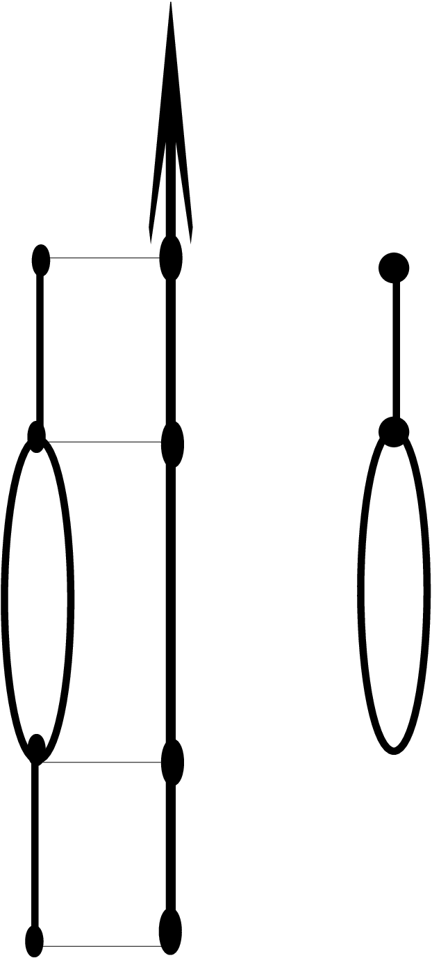
It is obvious that a graph has a good function if and only if it has no loops.
Next, we construct local functions around vertices respecting the value of the given good function at each vertex. Last we construct a local function having no singular points around each connected component of the complementary set of the disjoint union of small neighborhoods of vertices.
In the present paper, we show the following result. Several undefined terminologies and notation will be explained in the next section.
Theorem 1.
Let be a finite and connected graph which has at least one edge and has a good function . Suppose that a non-negative integer is assigned to each edge. Then there exist a -dimensional closed, connected and orientable manifold and a smooth function on satisfying the following properties.
- (1)
The Reeb graph of is isomorphic to : we can take an isomorphism .
- (2)
If we consider the natural quotient map and for each point () that is not a vertex and that is in an edge an integer is assigned to, then the preimage is a closed and orientable surface of genus .
- (3)
For a point mapped by the quotient map to a vertex , .
- (4)
At each singular point, the function is represented as a Morse function, a composition of a submersion with a Morse function, or a composition of a fold map with a Morse function. Moreover, for the latter two cases, the Morse functions are height functions of a line or an open ball of dimension .
- (5)
Furthermore, we can construct so that the restriction to the preimage of the interior of a small regular neighborhood of vertex of degree of (for the map ) is represented as a composition of a fold map with a height function of an open ball of dimension . Furthermore, the fold map is constructed as a map (as presented in FIGURE 6) satisfying the following three.
- (a)
Each connected component of the preimage of each point in the target is a circle, a bouquet of two circles, or a -dimensional polyhedron obtained in the following way.
- (i)
Choose a suitable integer and take copies of a circle.
- (ii)
For two of the copies, choose exactly one point for each copy, denoted by and .
- (iii)
For the remaining copies, choose exactly distinct points for each copy and for the -th copy, denoted by and .
- (iv)
Identify and for each .
- (i)
- (b)
For the singular set of the fold map, remove finitely many singular points and consider the restriction there. This is an embedding.
- (c)
The finitely many singular points removed before are in a same preimage.
- (a)
We prove this in the next section. We construct a desired function by the presented method. A new ingredient in the proof is construction around vertices at which the function has local extrema, or STEP 2. We end the paper by presenting related new problems or Problems 2 and 3, Remark 3, explaining relation between studies of the present paper and those in [17], and Remark 4.
2. Several terminologies and the proof of Theorem 1
Throughout the paper, denotes the -dimensional Euclidean space. For , denotes the distance between the origin and where the underlying metric is the Euclidean metric. denotes the -dimensional unit sphere and denotes the -dimensional unit disc.
For a smooth map, the singular value is a point such that the preimage contains a singular point. We define the set of all singular values of the map as the singular value set and the regular value set as the complementary set of the singular value set. A point in the regular value set of the map is said to be a regular value, which is explained before. Morse functions are well-known but we will refer to them in the presentation of a fold map later. We also note that height functions of (open) disks are simplest examples of Morse functions and we consider such functions in various cases in this paper.
A smooth map from a manifold of dimension with no boundary into a manifold of dimension with no boundary is said to be a fold map if the relation holds and at each singular point , there exists an integer satisfying and the map is represented as for suitable coordinates. The case where the target is is for Morse functions. So-called natural height functions of (open) disks before are Morse functions with exactly one singular point with . Note also that a correspondence of handle attachments to level sets of Morse functions and singular points of Morse functions is well-known. This fact gives us keys in various situations in geometry including several arguments of the present paper. Related to this and fundamental arguments on Morse functions, see [12] for example.
Proposition 1.
For a fold map just before, the following two properties hold.
- (1)
The integer is unique (we call the index of ).
- (2)
The set of all singular points of an index is a closed smooth submanifold of dimension with no boundary and the map obtained by restricting the original map to the set is an immersion.
In other words, a fold map is locally regarded as a product of a Morse function with exactly one singular point and the identity map on an open ball. We can also see this by virtue of a kind of Thom’s second isotopy lemma (see the proof of Theorem 5.1 of [18] and so on for explicit usages of such a lemma to see that a given smooth map is regarded as a product map of another smooth map and a suitable identity map on an open disk). See also FIGURE 2.

For fundamental singular theoretical and differential topological properties of fold maps, see [5], [14], [15] and so on.
We introduce the rigorous definition of the Reeb space (graph) of a smooth function. Let be a smooth manifold of dimension and be a smooth function. We define a relation on by the following rule: if and only if and are in a same connected component of a preimage . This is an equivalence relation on and we can define the quotient space .
Definition 1.
is said to be the Reeb space of .
We denote the quotient map by .
We define contains some singular point of . .
Definition 2.
If we can regard as a graph whose vertex set is , then is said to be the Reeb graph of .
Remark 1.
Reeb spaces may not be regarded as graphs generally ([17]): the present paper concentrates on smooth functions with finitely many singular values and Reeb spaces are Reeb graphs.
Remark 2.
Most of functions obtained in the present paper are of the class of Morse-Bott functions (if we remove finitely many singular points). For Morse-Bott functions see [1] for example.
We prove Theorem 1. Hereafter, for a finite set , denotes the cardinality of .
A proof of Theorem 1.
STEP 1 Construction around a vertex at which does not have a local extremum.
We demonstrate construction presented in [7], which is also based on methods in [9], [10] and [19].
We will construct a local Morse function with exactly one singular value respecting so that preimages of points in the regular value set are desired connected and orientable surfaces and that the Reeb space is as desired. We introduce notation.
- (1)
Let be the set of all edges containing the vertex such that on each edge has the value smaller than or equal to . Let be the disjoint union of closed, connected and orientable surfaces such that the genus of each surface and the integer attached to the corresponding edge coincide.
- (2)
Let be the set of all edges containing the vertex such that on each edge has the values greater than or equal to . Let be the disjoint union of closed, connected and orientable surfaces such that the genus of each surface and the integer attached to the corresponding edge coincide.
This covers all cases we need.
First we consider the case where the numbers assigned to the edges are all . For real numbers and satisfying , we can construct a desired function and a suitable homeomorphism from the resulting Reeb space of the local function to a small regular neighborhood of satisfying the following five by virtue of section 4 (Lemma 4.1) of [10] together with fundamental theory of Morse functions and handle attachments.
- (1)
The image of the function is and this function has finitely many or singular points and singular values are always .
- (2)
On the interior they are Morse functions with finitely many singular points.
- (3)
and the small regular neighborhood of are regarded as graphs having exactly edges, which are all originating from and respectively, and exactly vertices including exactly vertices of degree .
- (4)
The preimage of is diffeomorphic to and that of is diffeomorphic to .
- (5)
The preimage of the singular value is homeomorphic to a connected polyhedron obtained in the following way. Take finitely many copies of and let the number of copies. Take a suitable integer and disjoint points there. We divide the set of these points into pairs. We identify the points for each pair of the points.
Let be a real number satisfying . Before we consider general cases, we need to define smooth functions and on a -dimensional compact, connected and orientable manifold whose boundary is diffeomorphic to the disjoint union of a copy of the -dimensional unit sphere and a copy of satisfying the following properties. These functions are compositions of a copy of a Morse function with suitable diffeomorphisms on the targets and the characters ”” and ”” in the functions mean ”increasing” and ”decreasing” respectively: the orientations for the functions are mutually upside down.
- (1)
The images of these functions are and these functions have exactly one singular point.
- (2)
On the interior they are Morse functions with exactly one singular point and the singular values are both .
- (3)
and the connected component of the boundary diffeomorphic to agree. and the connected component of the boundary diffeomorphic to agree.
- (4)
and the remaining connected component of the boundary, diffeomorphic to , agree. and the remaining connected component of the boundary, diffeomorphic to the torus, agree.
We can remove the interiors of two disjoint compact and smooth manifolds the restrictions of the original functions to which give trivial smooth bundles over whose fibers are diffeomorphic to by virtue of (a relative version of) Ehresmann’s fibration theorem ([2]). After that, we can have functions and satisfying the following four properties.
- (1)
They are restrictions of the original functions.
- (2)
Their images are both and their Reeb spaces are both homeomorphic to a closed interval.
- (3)
They have exactly one singular point and the singular values are both .
- (4)
and are diffeomorphic to .
- (5)
and are diffeomorphic to a compact, connected and orientable surface of genus with one hole (or the torus with one hole).
See also FIGURE 3.

We will discuss a general case. For an arbitrary pair of positive integers, we can construct the desired function in the case .
We construct a desired function by removing the interiors of finitely many disjoint compact and smooth manifolds the restrictions of the function to which give trivial smooth bundles over whose fibers are diffeomorphic to and attach finitely many copies of or for a small preserving the values of the functions instead.
We can do this and take a homeomorphism from the resulting Reeb space of the local function to a small regular neighborhood of so that the following four properties hold: essentially (a relative version of) Ehresmann’s fibration theorem and the structures of the original -dimensional manifold and the original function enable us to do this. Let the function on corresponding the integers assigned to the edges denote by .
- (1)
and the regular neighborhood of are regarded as graphs having exactly edges, which are all originating from and respectively, and exactly vertices including exactly vertices of degree .
- (2)
The number of copies of we use to construct the desired function is .
- (3)
The number of copies of we use to construct the desired function is .
- (4)
The number of the copies of the subset of the domain of above mapped to an edge by such that is an edge of the small regular neighborhood of and also in a unique edge of the graph is .
- (5)
The number of the copies of the subset of the domain of above mapped to an edge by such that is an edge of the small regular neighborhood of and also in a unique edge of the graph is .
This completes the exposition of a desired function around .
Of course by the construction the five properties in Theorem 1 hold. Note that we may ignore the last property in STEP 1.
This completes STEP 1.
Hereafter, in the local construction as before we omit precise expositions as before using a suitable homeomorphism from the resulting Reeb space of the local function to a small regular neighborhood of .
STEP 2 Construction around a vertex at which has a local extremum.
CASE 1 The case where the vertex is of degree larger than .
We divide the set of all the edges containing the vertex into two non-empty sets and . Let be a closed surface obtained as the disjoint union of all closed, connected and orientable surfaces the genius of each of which is the number assigned to the corresponding edge in . For and , we construct a suitable local Morse function as STEP 1 so that preimages of regular values smaller than the singular value are diffeomorphic to and those of regular values greater than the value are diffeomorphic to . After this construction, we embed the image so that the image is a parabola in the plane and that the singular value is the local extremum with respect to the vertical component and compose a canonical projection to the vertical axis. The resulting local function is a desired function. We can see that this local function satisfies the first three properties in Theorem 1. For the fourth property, it is regarded as a composition of two Morse functions. At each singular point, the local function is represented as a composition of a submersion with a Morse function or a composition of a Morse function with a Morse function. In addition, in the two compositions, the latter Morse functions are natural height functions of a line.
For the construction, see also FIGURE 4.

CASE 2 The case where the vertex is of degree .
We first show the case where a positive integer is assigned to the edge containing the vertex.
Let be an integer, let be a real number and let be an increasing sequence of real numbers satisfying : if then and if then or . Let be a compact, connected and orientable surface obtained by removing the interiors of disjointly and smoothly embedded copies of a -dimensional standard closed disk in a -dimensional sphere. We have a smooth deformation of smooth functions defined as where are smooth functions on satisfying the following properties.
- (1)
The images of these functions are and these functions have exactly singular points.
- (2)
On the interior they are Morse functions with exactly singular points whose indices are and the singular value set of is .
- (3)
For , the preimage of a regular value in the lower bound of its singular value set is a circle and the preimage of a regular value in the upper bound of the singular value set is a disjoint union of circles.
- (4)
For and , the preimage of a regular value in is a disjoint union of circles. For and , the preimage of a regular value in is a disjoint union of circles.
- (5)
The preimage of each singular value of these functions is as follows.
- (a)
A disjoint union of finitely many copies of a circle and a bouquet of two circles in the case ().
- (b)
A -dimensional polyhedron obtained in the following way in the case ().
- (i)
Take circles.
- (ii)
For two of the copies, choose exactly one point for each copy, denoted by and .
- (iii)
For the remaining copies, choose exactly distinct points for each copy and for the -th copy, denoted by and .
- (iv)
Identify and for each .
- (i)
- (a)
- (6)
(The restriction of) (to the interior) is a fold map and the singular set of is a disjoint union of copies of a closed interval. If we restrict to each connected component of the singular set, then the resulting map is an embedding and the image is .
See also FIGURE 5. Note that this makes sense for .

Thus we have a local fold map from a -dimensional orientable manifold onto (by restricting the domain and the target of to the interiors). FIGURE 6 shows the image of the fold map. Thick lines intersect at the origin and these lines represent straight lines containing the origin consisting of values of the map at singular points whose indices are . If we go in the direction of the arrows in the plane, then the number of connected components of the preimages of regular values increases.
We restrict the map to the preimage of the disk bounded by the dotted circle in FIGURE 6 and let the target be this disk. We take the disk as for a (sufficiently small) positive number . Let the map on the -dimensional manifold onto the disk denote by .
The restriction of to the preimage of is a so-called circle-valued Morse map and this has exactly singular points. Their indices are all . We can see that the preimage of the embedded dotted circle is a closed, connected and orientable surface of genus . Note also that in cases where the numbers of the thick lines are or (or or ) or so-called generic cases, see [15] for example. The local map in a general case is also regarded as a generalization of these maps.

We consider a natural height function of the (interior of the) disk whose exactly one singular point is the origin (we can define the height function as a function represented as for suitable coordinates).
By composing the local fold map () on the -dimensional manifold into the (interior of the) disk with this height function, we obtain a local function such that the image and the Reeb space is homeomorphic to . Each point in the interior of the image is a regular value since the image of the rank of the differential of the fold map at each singular point is and the preimage is a closed, connected and orientable surface of genus . For this, note also that for the fold map into the plane (disk), the preimage of is a closed, connected and orientable surface of genus and that the image of the differential at each singular point mapped to a point or a singular value different from the origin is regarded as the unique straight line in the singular value set of the fold map containing the singular value. The resulting local function is, at each point in the preimage of , represented as a composition of a fold map into the plane with a height function of an open -dimensional disk.
This local function is a desired local function. For the functions and maps here, we can see that the fourth and fifth properties in Theorem 1 hold. For the fold map into the plane, the preimage of the origin may contain more than one singular point, where other preimages do not. As in CASE 1, we can see that this local function satisfies the first three properties in the theorem.
We must also show the case where is assigned to the edge containing the vertex. To make the preimage at the point in the interior of the edge diffeomorphic to , or equivalently, a closed, connected and orientable surface of genus , it is sufficient to consider a height function of an open -dimensional disk.
This completes the proof for CASE 2 and STEP 2.
STEP 3 Around each connected component of the complementary set of the disjoint union of small regular neighborhoods of vertices.
Last, we construct functions around each connected component of the complementary set of the disjoint union of small regular neighborhoods of vertices. We can construct these functions as trivial smooth bundles.
Finally, we can glue the local functions together by suitable diffeomorphisms. Note that several local functions in the present paper are constructed as functions on open manifolds with compact ends and we can extend them to smooth functions on compact manifolds with boundaries in canonical ways. Note also that we can choose the diffeomorphisms so that the manifolds are orientable. This gives a desired function on a -dimensional closed, connected and orientable manifold and we also have a desired isomorphism between the graphs by gluing in a natural way. This completes the proof.
∎
Problem 2.
Find restrictions on the topologies of manifolds admitting functions of Theorem 1 satisfying appropriate topological conditions.
As a simplest answer, in [16], manifolds admitting Morse functions such that preimages of regular values are disjoint unions of a copy of have been studied for . As another simplest result, it has been shown that a -dimensional closed, connected and orientable manifold admits a Morse function such that connected components of preimages of regular values are always diffeomorphic to or if and only if it is diffeomorphic to or represented as a connected sum of Lens spaces or copies of . In other words, the case where or are assigned to all edges of the graphs in Theorem 1 was studied there under the additional constraint that the class of functions is restricted to the class of Morse functions. See also Remark 3.
Problem 3.
Can we show a non-orientable version of Theorem 1?
The author has a positive idea and an answer will be presented in a forthcoming paper.
Remark 3.
[17] is regarded as a related work motivated by the present paper. This concerns a general case where preimages of regular values are arbitrary compact manifolds possibly with boundaries of a fixed dimension. In the work explicit singularities of smooth functions are not studied: only so-called bump functions are used in constructing global functions for example. In the present paper an explicit class of smooth functions on -dimensional closed, connected and orientable manifolds is studied where such very explicit cases are not studied in [17].
Note that for example if we restrict our functions to functions with finitely many singular points then they are Morse functions whose singular values may agree at distinct singular points. Related to this, note also that in the answer to Problem 2 presented just before, such a restriction of the class of functions restrict the class of manifolds admitting functions of the class to the presented class of -dimensional manifolds. Furthermore, if we do not restrict the class of functions of Theorem 1 and we pose the condition that to all edges of the given graph or are assigned only, then we do not know the class of manifolds admitting functions of the class. Understanding this class seems to be difficult.
3. Acknowledgement.
The author would like to thank Professor Irina Gelbukh for invaluable comments given after the submission of an earlier version of the present paper to arXiv.org e-Print archive (https://arxiv.org/). One of the comments let the author think Problem 2 as a fundamental and important problem. She also kindly told the author about [3] and [4].
The author is a member of the project JSPS KAKENHI Grant Number JP17H06128 ”Innovative research of geometric topology and singularities of differentiable mappings”
and this work is supported by this project. The author would like to thank Osamu Saeki and colleagues in this project. The author can present several stuffs in the present paper owing to their comments in an informal seminar on the present paper. The author would like to thank Osamu Saeki for publishing [17] as a related work and an informal discussion on this.
The author would like to thank anonymous referees, who improved the quality of the present paper.
References
- [1] R. Bott, Nondegenerate critical manifolds, Ann. of Math. 60 (1954), 248–261.
- [2] C. Ehresmann, Les connexions infinitesimales dans un espace fibre differentiable, Colloque de Topologie, Bruxelles (1950), 29–55.
- [3] I. Gelbukh, Loops in Reeb graphs of -manifolds, diskrete & Computational Geometry, 59 (4) (2018), 843–863.
- [4] I. Gelbukh, Approximation of Metric Spaces by Reeb Graphs: Cycle Rank of a Reeb Graph, the Co-rank of the Fundamental Group, and Large Components of Level Sets on Riemannia manifolds, Filomat (in press), arxiv:1903.00777.
- [5] M. Golubitsky and V. Guillemin, Stable Mappings and Their Singularities, Graduate Texts in Mathematics (14), Springer-Verlag(1974).
- [6] N. Kitazawa, Smooth maps compatible with simplicial structures and preimages, arxiv:1802.06381v6.
- [7] N. Kitazawa, Structures of cobordism-like modules induced from generic maps of codimension -2, arxiv:1901.04994v1.
- [8] J. Martinez-Alfaro, I. S. Meza-Sarmiento and R. Oliveira, Topological classification of simple Morse Bott functions on surfaces, Contemp. Math. 675 (2016), 165–179.
- [9] Y. Masumoto and O. Saeki, A smooth function on a manifold with given Reeb graph, Kyushu J. Math. 65 (2011), 75–84.
- [10] L. P. Michalak, Realization of a graph as the Reeb graph of a Morse function on a manifold. Topol. Methods Nonlinear Anal. 52 (2) (2018), 749–762, arxiv:1805.06727.
- [11] L. P. Michalak, Combinatorial modifications of Reeb graphs and the realization problem, Discrete & Computational Geometry 65 (2021), 1038–1060, arxiv:1811.08031.
- [12] J. Milnor, Lectures on the h-cobordism theorem, Math. Notes, Princeton Univ. Press, Princeton, N.J. 1965.
- [13] G. Reeb, Sur les points singuliers d´une forme de Pfaff complétement intègrable ou d´une fonction numérique, Comptes Rendus Hebdomadaires des Séances de I´Académie des Sciences 222 (1946), 847–849.
- [14] O. Saeki, Notes on the topology of folds, J. Math. Soc. Japan Volume 44, Number 3 (1992), 551–566.
- [15] O. Saeki, Topology of singular fibers of differntiable maps, Lecture Notes in Math., Vol. 1854, Springer-Verlag, 2004.
- [16] O. Saeki, Morse functions with sphere fibers, Hiroshima Math. J. Volume 36, Number 1 (2006), 141–170.
- [17] O. Saeki, Reeb spaces of smooth functions on manifolds, Intermational Mathematics Research Notices, maa301, https://doi.org/10.1093/imrn/maa301, arxiv:2006.01689.
- [18] O. Saeki and M. Takase, Desingularizing special generic maps, Journal of Gokova Geometry Topology 7 (2013), 1–24.
- [19] V. Sharko, About Kronrod-Reeb graph of a function on a manifold, Methods of Functional Analysis and Topology 12 (2006), 389–396.