RTNI – A symbolic integrator for Haar-random
tensor networks
Abstract.
We provide a computer algebra package called Random Tensor Network Integrator (RTNI). It allows to compute averages of tensor networks containing multiple Haar-distributed random unitary matrices and deterministic symbolic tensors. Such tensor networks are represented as multigraphs, with vertices corresponding to tensors or random unitaries and edges corresponding to tensor contractions. Input and output spaces of random unitaries may be subdivided into arbitrary tensor factors, with dimensions treated symbolically. The algorithm implements the graphical Weingarten calculus and produces a weighted sum of tensor networks representing the average over the unitary group. We illustrate the use of this algorithmic tool on some examples from quantum information theory, including entropy calculations for random tensor network states as considered in toy models for holographic duality. Mathematica and Python implementations are supplied.
1. Introduction
The probabilistic method – made famous by Paul Erdös [Erd47] – now pervades all of discrete mathematics and computer science. In its most well-known form, it is used to demonstrate the existence of certain combinatorial objects by defining a suitable probability space, and showing that randomly chosen elements of that space exhibit the required property with non-zero probability. A prime example of this strategy is the proof of the achievability part of the channel coding theorem by Shannon [Sha48] in classical information theory, established roughly at the same time: here the method is applied to show the existence of capacity-achieving codes for a given communication channel. To mention just one additional famous example beyond the original applications to graph theory, the probabilistic method has been used to estimate sizes of -nets (respectively -samples) in spaces with limited Vapnik-Chervonenkis-Dimension [VC71].
While the probabilistic method constitutes a powerful mathematical tool, much more direct manifestations of randomness in the real world have been studied throughout the history of physics. Here we are particularly interested in the appearance of random matrices. The consideration of random matrices was initiated by Wigner in order to explain universal features of the eigenvalue spacing of atomic spectra [Wig55], but has since then gone undergone significant developments – see e.g., [GMGW98] for an in-depth review. Significant fields of application include the theory of disorder and associated transport phenomena in condensed matter systems, and the development of random matrix models in quantum field theory.
Random matrices, and more specifically the Haar distribution over a compact Lie group, also play a central role in quantum mechanics because of conservation laws. For example, any physical process respecting certain superselection rules can be described by a quantum channel (a completely positive trace-preserving map) which is covariant under the relevant group action. Thus such a channel can be seen as the result of “supertwirling”, i.e., the consequence of averaging (the inputs and outputs of) a given channel over the unitary group. Because this averaging operation typically leads to a drastic reduction of the number of free parameters, the set of covariant operations (and states) has often been a fruitful testbed and source of examples, e.g., in entanglement theory [Wer89]. Covariant channels (or instruments) also appear e.g., when considering certain operational figures of merit which are related for example to average fidelities (with averages taken over the Haar measure). In certain cases, the associated optimization problem can then be restricted to operations respecting the underlying symmetry. For example, optimal cloning devices where constructed following this approach in [Wer98, KW99]. We note that these are only some of the pioneering contributions to this area.
Interestingly, random matrices are fundamental to quantum information theory even beyond such symmetry considerations. Indeed, it was found that the probabilistic method can be used to establish existence (and it some cases “genericity”) of states and operations with particular properties; here the distributions are typically defined in terms of Haar-random unitaries. Pioneering work in this direction [HLSW04, HLW06] has shown for example the existence and ubiquity of states with a large amount of “locked” classical correlations. The probabilistic method was also used by Hastings [Has09b] to disprove the additivity conjecture for the Holevo-quantity: following a proof strategy successfully applied for Rényi entropies earlier [HW08, CHL+08] he demonstrated the existence of a pair of quantum channels for which the Holevo-quantity (which determines the classical capacity) is non-additive. Closer to the spirit of Shannon’s achievability theorem, the probabilistic method has also been used to show the achievability of the quantum capacity (more precisely, the coherent information): here the argument involves picking a random subspace respectively vectors (according to the Haar measure) of a Hilbert space [HHWY08, HSW08]. The corresponding “decoupling approach” is now a standard procedure in quantum information theory.
We refer to [CN16] for a detailed review of applications of random matrix techniques in quantum information theory. In most of these applications, averages are taken over the unitary group on some finite-dimensional space. Typically, one is interested in the moments of some expression (such as a matrix product) involving instances of random unitaries, and these are evaluated in an ad-hoc manner. In recent applications, random tensor network states are considered: here Haar-random unitaries are contracted together with fixed tensors in a network. An example is the consideration of random matrix product states [CGGPG13], and, more recently, the contraction of higher-dimensional random tensor networks in the context of holographic duality [HNQ+16] (see Example 6.5 below). In these cases, the evaluation of Haar averages of quantities of interest becomes highly non-trivial, either because higher moments are required, and/or because the average is over a -tuple of independently and identically distributed unitaries.
2. Our contribution
Our work is motivated by the ubiquity of Haar-random averages in a large variety of settings, and the fact that the associated computations are – on a conceptual level – very similar. Indeed, the natural language capturing these problems is that of random tensor networks: these allow to capture a variety of mathematical objects/expressions involving random matrices, including matrix products, tracial expressions, and tensor contractions. Furthermore, expectation values of such random tensor networks are themselves linear combinations of tensor networks (which may represent scalars, matrices or tensors), and – for Haar-random unitaries – these expectation values can be computed algorithmically using the Weingarten calculus.
Even though detailed derivations of the Weingarten calculus can be found in the literature, there appears to be no general implementation relying on symbolic manipulation of tensor networks. Our Random Tensor Network Integrator (RTNI) package11 1 Code available at https://github.com/MotohisaFukuda/RTNI aims to fill this gap by providing routines for computing expectation values of tensor networks involving random unitaries. This is envisioned to facilitate the study and application of objects involving Haar-random unitaries.
Let us briefly mention existing similar software packages dealing with Weingarten integration we are aware of. The IntU package [PM17] is a Mathematica package used for the computation of the averages monomials in the entries of a random unitary matrices, see also https://zksi.iitis.pl/wiki/projects:intu. There are two main differences with our implementation. Most importantly, we allow for symbolic Hilbert space dimensions, where as in IntU these dimensions must be fixed numerical integers. Moreover, our input data is a graph, as opposed to a monomial for IntU; we consider our input format more practical, especially for applications of the Weingarten calculus (and additionally provide subroutines for monomials). The IntHaar package [GK16] is a MAPLE implementation for the Weingarten calculus, see http://sites.math.rutgers.edu/~ag930/Maple%20Packages/IntHaar.txt for the code. Similarly to the IntU package, the program computes averages of polynomials in the entries of the random unitary matrix, but the Weingarten functions are computed symbolically. Moreover, the case of Haar-distributed orthogonal and symplectic matrices is implemented.
Outline
This document describes the RTNI package. In Section 3, we briefly review the underlying Weingarten formula. In Section 4, we recall the graphical Weingarten calculus which is realized by the RTNI package. Section 5 discusses the main routines provided by RTNI and their use. Finally, in Section 6, several explicit example computations are provided, illustrating the use of the package.
3. Mathematical background: the Weingarten formula
Here we briefly review the definition of some relevant mathematical objects, including, in particular, the Weingarten function. We defer the discussion of the graphical Weingarten calculus to Section 4 and instead begin with an “element-wise” expression of the Weingarten formula. This shows how to compute the average of monomials composed of matrix elements of random unitary matrices with respect to the Haar measure. This problem was first considered in the physics literature by Weingarten [Wei78] in the asymptotic limit of large dimension. An explicit expression for fixed matrix dimensions was obtained in [Col03] and [CŚ06] by Collins, respectively Collins and Śniady. The main insight exploited in those works is that the average of tensor product operators of the form is a weighted sum of permutation operators. This is a consequence of Schur-Weyl duality.
Theorem 3.1.
Let be positive integers and , , , be -tuples of positive integers from . Then
| (1) |
If then
| (2) |
Here we denoted by the unitary group acting on an -dimensional Hilbert space, and the integrals are taken with respect to the normalized Haar measure on . The function is called the unitary Weingarten function, see Definition 3.2 below.
We note that software packages such as the IntU package [PM17] mentioned above primarily rely on expression (1). In contrast, our RTNI package exploits the graphical calculus introduced in the next section, including, in particular, expression (11) below.
The unitary Weingarten function is a combinatorial object defined as follows. Let be the algebra of complex-valued functions on the symmetric group with product given by the convolution
| (3) |
The Dirac-Delta function for is the identity element in . For any , let be defined
| (4) |
where denotes the number of cycles of the permutation . Then belongs to the center .
Definition 3.2.
The unitary Weingarten function
| (5) | ||||
| (6) |
is a function of a dimension parameter and of a permutation . It is defined as the pseudo-inverse of the element defined in (4), i.e., the unique element in satisfying
| (7) |
It can be shown that if , then and are inverses of each other
| (8) |
Furthermore, for integer , the Weingarten functions can be written as
| (9) |
Here, means that is a partition of the integer , is the character of the irreducible representation of the symmetric group specified by , and is the Schur polynomial evaluated at the identity (i.e., the dimension of the irreducible representation of with highest weight . The latter is given by the formula
| (10) |
For integer , the element has no inverse, and formula (9) no longer applies, but a separate formula is needed. Indeed, expression (9) has poles when . However, in computing averages over the Haar measure as in Theorem 3.1, those poles cancel, yielding a rational function in on the RHS of (1). This is why one can use the expression of Eq. (9) for the Weingarten function for all in the computations as in Theorem 3.1. We refer to [CŚ06] for more details.
4. Graphical notation for tensors and for the Weingarten formula
In this section, we briefly recall the graphical calculus method for computing unitary integrals introduced in [CN10], to which the readers are referred for more details. As discussed below, the RTNI package provides a general implementation of this method.
First, we explain the graphical formalism for tensor calculus, which can be traced back to Penrose [Pen71]; for modern presentations, see [CN10] or [Coe10]. The main object here is a complex vector space of diagrams. An element of this vector space will be represented as a list of pairs of the form , where is a graph (a.k.a. a diagram or tensor network) and is a scalar weight; the corresponding element is . The diagrams (or graphs) correspond to tensors, and consist of boxes and wires. Boxes in a graph represent tensors. Each box has attached to it symbols of different shapes, where each shape corresponds to a vector space; identical shapes depict isomorphic vector spaces. Those symbols are filled (black) or empty (white), corresponding to primal or dual spaces. Wires connect these symbols, corresponding to tensor contractions . This is why each wire must connect symbols of the same shape, i.e. the same dimension. A diagram is a collection of such boxes and wires and corresponds to an element in a tensor product space. If there is more than one connected component in a graph, then the components are multiplied by taking the tensor product.
For example, the tensor (here, a bipartite matrix) , where stands for the partial trace over the first space, is represented in Figure 1. Consider the primal side of the box for the matrix . There are two symbols of different shapes implying that the effective primal space of is the tensor product of these two spaces.
Next, we describe how to efficiently compute expected values of diagrams which contain boxes of random unitary matrices. This technique in fact can be extracted from Theorem 3.1, once one uses the fact that the averaging process is linear. More precisely, the delta functions in each term in the RHS of (1) simply indicate how one needs to reconnect boxes corresponding to the random unitary operator and . For each pair of permutations in (1), one eliminates and boxes and reconnects the wires originally connected to these boxes to get a new diagram. Since these manipulations are made on wires and symbols (boxes), one can regard them as operations on a graph, identifying wires and symbols with edges and vertices, respectively. This process for a fixed pair of permutations is called a removal and the whole process which sums all the new graphs over all permutations is called the graph expansion. Formally, if is a diagram containing boxes corresponding to a Haar-distributed random unitary matrix , then its expectation value (with respect to ) is
| (11) |
where is the diagram obtained from by removing the boxes associated with and and adding extra wires to the resulting diagram, as follows: we connect white decorations of the -th box with the white decorations of the -th box and, by a similar procedure, the black decorations are paired using the permutation. One can see how this works in examples in Section 6, see in particular Figures 4 and 7.
5. The RTNI package
In this section, we explain how to use the RTNI package, available at https://github.com/MotohisaFukuda/RTNI. Readers are also referred to some examples in Section 6 while reading this section.
The following two functions are the main routines provided by RTNI:
- (1)
: integrates out the random unitary matrix in the tensor networks in .
- (2)
: produces a graphical output representing each tensor network (graph) in the list, together with the associated weights.
In Sections 5.1 and 5.2, we provide a detailed explanation of the functionality realized by these routines, as well as the syntax used for inputs and outputs. These two routines are the only routines needed for working with random tensor networks.
We also provide an additional auxiliary routine for matrix products, which covers many simple use-cases. It internally creates a tensor network representing the matrix product (respectively its trace), invokes integrateHaarUnitary, and re-expresses the resulting linear combination of tensor networks in terms of matrix products/tracial expressions.
- (3)
: symbolically computes moments of matrix products involving Haar-random unitaries.
The corresponding syntax is explained in Section 5.3.
5.1. integrateHaarUnitary
An input of integrateHaarUnitary specifies the diagrams (tensor networks) containing random matrices to be averaged. At the program level, inputs of the function integrateHaarUnitary divide into five variables as indicated above. In the following, we describe each of them.
- (1)
TNList is a list of pairs (tnsj,weightj) represeting a weighted linear combination of (with arbitrary) tensor networks, where the -th tensor network tnsj has weight weightj. The syntax is as follows:
{{tns1, weight1 }, { tns2, weight2 },…, { tnsn, weightn } }
For (i.e., if only one tensor network is considered) and the associated weight is equal to , the alternative expression
tns
may be used. In these expressions, each term “tns” is a list of edges of the form
{{vertex, vertex }, …, { vertex, vertex } }
and “weight” is a symbolic expression or scalar specifying the weight of the associated tensor network.
Vertices correspond to the different shaped and colored decorations attached to boxes in the graphical calculus from Section 4. Importantly, each term “vertex” is given by a list of four items in the format
{varName, ID, IN/OUT, leg}
where
- •
varName is a string denoting the name of the corresponding box; for boxes associated to Haar random unitary matrices, this string can end in the star symbol “”, in which case this references the adjoint of the unitary operator.
- •
ID is an integer used to distinguish between several copies of the same box; this is in particular used to distinguish different copies of random unitary matrices and their adjoints.
- •
IN/OUT is a string, referring to whether the vertex corresponds to an input (”in”) or an output (”out”) of a matrix.
- •
leg is a positive integer corresponding to which tensor factor the vertex corresponds to.
We display in Figure 2 an example of a tensor network; the three edges appearing are encoded by (from left to right, and top to bottom; the colors are used for clarity only):
Figure 2. A tensor network containing three edges (wires). The -boxes on the left have IDs 1 and 2 (labels in the bottom-right corner of the boxes), while occurs only once (and the ID 1 is used) and has two legs numbered 1 and 2, respectively (labels near the decorations of the box). Output vertices are marked by filled circles, whereas input vertices are marked by empty circles. The edges also carry labels, to make their encoding more clear. - •
- (2)
varName is a letter showing over which random matrix the tensor network (respectively linear combination of tensor networks) is to be averaged.
- (3)
inDims is a list specifying the dimensions of the factors in the tensor product corresponding to the outputs of the random unitary matrix.
- (4)
outDims is a list specifying the dimensions of the factors in the tensor product corresponding to the inputs of the random unitary matrix.
- (5)
totalDims is the size of the random unitary matrix to be integrated out.
It is important to note that the elements of the lists outDims, inDimns, as well as totalDims can be symbolic.
An output of integrateHaarUnitary is a list made of pairs of tensor networks and weights:
{{tns1, weight1 }, { tns2, weight2 },…, { tnsm, weightm } }
Hence the output can be fed into integrateHaarUnitary for iterative calculations. Note that integrateHaarUnitary creates new edges (and new vertices): these correspond to symbols on the random matrix which are not connected to other symbols (which did not appear in TNList). In the Mathematica package the names of such new vertices starts with “dummy”, and in the Python package with “@”. One can also add such extra vertices manually.
5.2. visualizeTN
As the name indicates, this function creates a graphical representation of a single tensor network respectively a weighted list of tensor networks. An input of visualizeTN is the first argument of an input, or an output of integrateHaarUnitary. An example is shown in Fig. 3. The arguments are as follows:
- (1)
TNList This is either a single tensor network, or a list of (weighted) tensor networks as in the description above.
- (2)
{EdgeLabeling True} This optional second argument forces the visualization to display edge labels, indicating which input/output is connected to which input/output. This argument can be omitted, in which case edges are not labeled.
5.3. MultinomialexpectationvalueHaar
An input of MultinomialexpectationvalueHaar specifies a “matrix product” expression of the form
| (12) |
where each is either a fixed unitary , its Hermitian adjoint , its transpose , or its entriwise complex conjugate . The function takes an additional dimension parameter and computes the Haar averaged expression symbolically. In more detail, the input variables are the following:
- (1)
Dim is (a symbolical expression giving) the dimension of the matrices that are integrated over.
- (2)
eList is a list of the form (for any integer ). Here for each . Here the values define the unitary part of the expressions (12) by the following translation table:
1 2 3 4 - (3)
variableList is a list of the form . Here the -term directly specifies the -th variable in an expression of the form (12)
- (4)
usetrace is either or . It determines whether the first or second term in (12) is computed according to the table
usetrace expression computed
The output of “MultinomialexpectationvalueHaar” is a symbolic expression giving corresponding Haar average. Examples for this function are given in Section 6.6.
5.4. Weingarten functions and precomputed values
A table of precomputed Weingarten function is loaded upon program initialization. These are produced by a program in the Python package, and are stored in a subdirectory called precomputedWG. The latter computes all values of Weingarten functions based on expression (9). At present, all Weingarten functions with are provided, with being a symbolic parameter. In particular, this means that the Mathematica package can only compute averages of tensor networks containing up to boxes corresponding to a random unitary matrix of some type (and the corresponding number of conjugate/adjoint boxes).
5.5. Differences between the Mathematica and Python packages
There are two implementations for Mathematica and Python, but they work almost identically from the user’s viewpoint, with the replacement of curly brackets (Mathematica) with square brackets (Python).
In the Mathematica package, it is possible to give as an input a single diagram, in which case the function assigns it the weight 1, as specified above. This feature is not implemented in Python.
In the Python package, the input of the routine integrateHaarUnitary is of the form (TNList, randomMatrixList), where
- (1)
TNList is a (weighted) list of tensor networks as above, and
- (2)
randomMatrixList is a list of the form
[ [varName, outDims, inDimns, totalDims], …, [varName, outDims, inDimns, totalDims] ]
The routine then computes the average of a tensor network over multiple random unitary matrices at once. In contrast, in Mathematica, the routine needs to be invoked several times.
The Mathematica package loads the (provided) precomputed values of the Weingarten functions. The Python routine first checks if there is a preexisting set of precomputed Weingarten function for as required. If not, this is computed and saved to the folder named “Weingarten”. To this end, the Python package also creates folders named “SGC” and “SP” which contain the characters of symmetric groups and Schur polynomials. See Appendix B for more details.
6. Examples
Here we present a collection of simple examples of use cases for the package RTNI. We gradually work our way up from basic situations to more involved cases, presenting the code (of the Mathematica implementation) and comparing with analytical computations.
6.1. Twirling a matrix
We start with the simplest possible example, which is to compute the overlap between a fixed matrix and a “twirled” matrix , where is a fixed matrix and is a Haar-distributed random unitary matrix (also of size ). The result is a scalar
The diagram corresponding to the integral above, and its Weingarten expansion are depicted in Figure 4; the result is
| (13) |
In order to implement this in the RTNI package, we first need to input the corresponding tensor network (see Figure 4 top): it is a square, having 4 edges.
The tensor network described by this code is visualized on the left in Figure 5, using the subroutine visualizeTN; it is essentially identical to Figure 4. The four edges correspond to the four matrix products in the trace. Let us analyze in detail the first edge, . Its source is the -box having ID 1 (there is only one such box, i.e. occurs only once in the diagram), and more precisely it is an “input” of that box (hence the ”in” in the third position of the list describing the source). Since there is just one vector space in this example, the fourth parameter is 1. The sink of is the output (the ”out” in the third position) of the first (the 1 in the second position) box; again, the last parameter is 1, indicating that we are using the first (and only) factor of the tensor product here. The tensor network is the collection of the four edges, and it is displayed using the function visualizeTN. Next, we perform the unitary integration, as follows:
The resulting weighted sum of tensor networks (in this case having only one summand) is then displayed using the routine visualizeTN, see the right subfigure of Figure 5. There are two single vertex loop graphs corresponding to the two traces and the Weingarten weight.
The command integrateHaarUnitary invoked above is the main routine of our package, and it performs the integral of the tensor network over the unitaries corresponding to the letter (these are the boxes and ), assigning, in order, dimensions to the input spaces of , the output spaces of , and the total dimension of (here, there is just one input/output space, and all the dimensions are equal to ). The output is a (weighted) list of tensor networks (just one in this case), and we recognize in Figure 5 the tensor network with one vertex () with one loop attached (corresponding to ), the trace of , and the weight of the tensor network, .
Next, we consider the same example but without the trace, i.e., the expression . Now, the result of the computation is no longer a scalar, but equal to
| (14) |
To compute this, the following code can be used:
In this case, the RTNI package creates a “dummy” vertex for the input of , in order to work with a proper tensor network. After the computation, this dummy vertex is connected to the output of , see Figure 6.
We note that both expectation values and considered here could alternatively be computed using the subroutine MultinomialexpectationvalueHaar, see Example 6.6 below.
6.2. Several tensor factors
We now consider an example where the random unitary operators are bipartite: they act on a tensor product space. More precisely, we are interested in the partial trace of a twirled operator
where the identity operator acts on a tensor factor (with label 1) of dimension , while the trace operator acts on a different tensor factor (with label 2) of dimension .
The analytical computation of the Weingarten integral with respect to is straightforward: the result reads
| (15) |
The corresponding tensor networks for both the expresssion and its expectation are illustrated in Fig. 7.
The Mathematica code for the corresponding tensor network and for the computation of the expectation value with respect to the bipartite unitary matrix is as follows. In this example, one needs to specify that the unitary matrices and act on a tensor product of two vector spaces with respective dimensions and . The input and output spaces are identical, and the total dimension is .
6.3. Bi-partite twirling
Bi- or multi-partite twirling is one of the most useful primitives in quantum information theory, when one has to do with some kind of permutational or rotational symmetry. Introduced by Werner in [Wer89], it has found many applications in the theory of quantum information. We shall be concerned here with the bi-partite case
| (16) |
where is a Haar-distributed random unitary matrix and is a fixed matrix on which the twirling map is acting. The Weingarten computation is more involved in this case, since we are dealing with two copies of the same random unitary matrix (we are in the case of formula (1)).
The analytical computation of the integral in (16) proceeds as follows. First, let denote the flip (or swap) operator, defined by
Then, the four choices of the permutations from (1) give four terms, as follows:
| \ | (1)(2) | (12) |
|---|---|---|
| (1)(2) | ||
| (12) |
Putting everything together, we obtain
The Mathematica code used to compute the twirling of an operator is below.
Note that the output list of (weighted) tensor networks consists of 4 tensor networks, corresponding, respectively, to the entries , , , of the table above. The input and output are illustrated in Figure 9.
6.4. Bell state as input in conjugate random quantum channels
In this section, we discuss an application of RTNI to the theory of random quantum channels. Consider a random quantum channel given by a random isometry ,
Such random quantum channels were first considered in [HW08] in relation to the additivity conjecture in quantum information theory, solved in the negative by Hastings [Has09a]. In such considerations, one bounds the minimum output entropy of the tensor product channel by using the overlap
| (17) |
between the output of the channels acting on a maximally entangled state with another maximally entangled state (on the output spaces) . Here is the complex conjugate channel. The diagram for the scalar is given in Figure 10. Recall that the maximally entangled state is defined, in general, by , with
| (18) |
where is a given orthonormal basis of . In [HW08], it was shown that, for all (random) isometries , . This bound was improved in [CN10], where it was shown that, in the asymptotic regime where is fixed, , and for some ,
| (19) |
We confirm this computation using our symbolic Weingarten integration routines; note that the corresponding edges are also represented in Figure 10.
Note that we obtain first a formula for at finite ; we then take the limit to recover (19).
6.5. Random tensor networks for holographic duality
In this section, we illustrate the versatility of the RTNI package on an example taken from [HNQ+16]. The authors of [HNQ+16] relate the entanglement properties of a model of random tensors to the AdS/CFT correspondence. In our treatment below, we shall consider a simplified version of their model of random tensors (to be precise, we shall not consider bulk states as in [HNQ+16, Section 2]) that will be analyzed on some example with the help of the RTNI routines.
To a given unoriented simple graph on vertices, we shall associate an -tensor , as follows. For a vertex of degree , consider a random pure state (unit vector)
where is a Haar-distributed random unitary matrix and is a fixed vector; moreover, assume that the family is independent. Among the tensor legs of , the first one is a dangling edge, while the remaining ones will be contracted with the neighboring vertices to give the state (see Figure 11 for the case of a triangle graph):
where is the maximally entangled state from (18).
For a fixed (possibly empty) subset , consider the marginal
It is important to note that neither nor are normalized quantum states; this is due to the fact that the tensor contractions implemented by the maximally entangled states are not isometries. We define the normalized version (we drop the index to make the notation lighter)
and we compute, as in [HNQ+16], its -Renyi entropy
where is the flip operator, is the (global) density operator, and denotes the flip operator acting on the sites associated with (respectively its copy ). In [HNQ+16] it is argued that both the numerator and the denominator of the expression above concentrate around their average value (with respect to the randomness in the Haar unitaries ), denoted in general by
| (20) |
In [HNQ+16, Section 2.2], the value of averages of the form (20) was shown to be expressible – to lowest order in the limit – in terms of the minimum energy associated with an Ising model with classical spins on the vertices of the graph , and a magnetic field determined by the sites of interest. More precisely, the following expression was derived:
| (21) |
where
Obviously, in the case where (which corresponds to the normalizing denominator for the state ), the unique optimum is , and we obtain
| (22) |
Here we use the RTNI package to verify the validity of (21) and (22) for simple example of graphs 22 2 In [HNQ+16], expressions (21) and (22) are subsequently used to derive Ryu-Takayanagi-type formulas for the Rényi entropy. We do not consider this here as this derivation appears to require additional assumptions on connectivity properties of the graph , guaranteeing the minimum-energy considerations have a single domain wall (unlike in triangle graph example considered here). . In the case of the triangle graph shown in Figure 11, with a single point marginal , we obtain again that the optimizing configuration is for all and thus we obtain from (22) and (21)
| (23) | ||||
| (24) |
This result is confirmed by the following RTNI exact, non-asymptotic, computation (see also Figure 12). Note that the pre-factor appears below to take into account the normalization of the maximally entangled states (18), which is not encoded directly into the tensor network.
Here the routine buildTNfromGraph creates two tensor networks starting from a graph and a subset of vertices. The tensor networks represent and , respectively (see Fig. 12). The corresponding code and additional examples for e.g., 2D grid graphs are provided in a separate Mathematica notebook.
6.6. Example computation of expectation values of matrix products
Here we illustrate the use of MultinomialexpectationvalueHaar. We use the routine to obtain
| (25) | ||||
| (26) | ||||
| (27) | ||||
| (28) |
for two -matrices and a Haar-random unitary of size .
For two additional matrices , we can compute for example
| (29) | ||||
| (30) |
using the command
Acknowledgments. I.N.’s research has been supported by the ANR projects StoQ ANR-14-CE25-0003-01 and NEXT ANR-10-LABX-0037-NEXT. I.N. and M.F. acknowledge the hospitality of the TU München, where part of this work was conducted, and are both supported by the PHC Sakura program (project number: 38615VA). R.K. acknowledges support by DFG project no. K05430/1-1 and the Technical University of Munich – Institute for Advanced Study, funded by the German Excellence Initiative and the European Union Seventh Framework Programme under grant agreement no. 291763. M.F. was financially supported by JSPS KAKENHI Grant Number JP16K00005.
References
- [Ber04] Dan Bernstein. The computational complexity of rules for the character table of . Journal of Symbolic Computation, 37(6):727 – 748, 2004.
- [CGGPG13] Benoît Collins, Carlos E. González-Guillén, and David Pérez-García. Matrix product states, random matrix theory and the principle of maximum entropy. Communications in Mathematical Physics, 320(3):663–677, Jun 2013.
- [CHL+08] Toby Cubitt, Aram W. Harrow, Debbie Leung, Ashley Montanaro, and Andreas Winter. Counterexamples to additivity of minimum output -Rényi entropy for close to 0. Communications in Mathematical Physics, 284(1):281–290, Nov 2008.
- [CN10] Benoît Collins and Ion Nechita. Random quantum channels I: graphical calculus and the Bell state phenomenon. Communications in Mathematical Physics, 297(2):345–370, 2010.
- [CN16] Benoît Collins and Ion Nechita. Random matrix techniques in quantum information theory. Journal of Mathematical Physics, 57(1):015215, 2016.
- [Coe10] Bob Coecke. Quantum picturalism. Contemporary physics, 51(1):59–83, 2010.
- [Col03] Benoît Collins. Moments and cumulants of polynomial random variables on unitarygroups, the itzykson-zuber integral, and free probability. International Mathematics Research Notices, 2003(17):953–982, 2003.
- [CŚ06] Benoît Collins and Piotr Śniady. Integration with respect to the haar measure on unitary, orthogonal and symplectic group. Communications in Mathematical Physics, 264(3):773–795, 2006.
- [Erd47] P. Erdös. Some remarks on the theory of graphs. Bull. Amer. Math. Soc., 53:292–294, 1947.
- [GK16] Alejandro Ginory and Jongwon Kim. Weingarten calculus and the IntHaar package for integrals over compact matrix groups. arXiv preprint arXiv:1612.07641, 2016.
- [GMGW98] Thomas Guhr, Axel Müller-Groeling, and Hans A. Weidenmüller. Random-matrix theories in quantum physics: common concepts. Physics Reports, 299(4):189 – 425, 1998.
- [Has09a] Matthew B Hastings. Superadditivity of communication capacity using entangled inputs. Nature Physics, 5(4):255–257, 2009.
- [Has09b] M.B. Hastings. Superadditivity of communication capacity using entangled inputs. Nature Physics, 5:255–257, March 2009.
- [HHWY08] Patrick Hayden, Michal Horodecki, Andreas Winter, and Jon Yard. A decoupling approach to the quantum capacity. Open Systems & Information Dynamics, 15(01):7–19, 2008.
- [HLSW04] Patrick Hayden, Debbie Leung, Peter W. Shor, and Andreas Winter. Randomizing quantum states: Constructions and applications. Communications in Mathematical Physics, 250(2):371–391, Sep 2004.
- [HLW06] Patrick Hayden, Debbie W. Leung, and Andreas Winter. Aspects of generic entanglement. Communications in Mathematical Physics, 265(1):95–117, Jul 2006.
- [HNQ+16] Patrick Hayden, Sepehr Nezami, Xiao-Liang Qi, Nathaniel Thomas, Michael Walter, and Zhao Yang. Holographic duality from random tensor networks. Journal of High Energy Physics, 2016(11):9, 2016.
- [HSW08] Patrick Hayden, Peter W. Shor, and Andreas Winter. Random quantum codes from gaussian ensembles and an uncertainty relation. Open Systems & Information Dynamics, 15(01):71–89, 2008.
- [HW08] Patrick Hayden and Andreas Winter. Counterexamples to the maximal -norm multiplicativity conjecture for all . Communications in Mathematical Physics, 284(1):263–280, 2008.
- [KW99] M. Keyl and R. F. Werner. Optimal cloning of pure states, testing single clones. Journal of Mathematical Physics, 40(7):3283–3299, 1999.
- [Mur71] Francis D. Murnaghan. The characters of the symmetric group. Proc. Nat. Acad. Sci. U.S.A., 68:399–401, 1971.
- [Nak41a] T. Nakayama. On some modular properties of irreducible representations of a symmetric group. I. Jap. J. Math., 18:89–108, 1941.
- [Nak41b] Tadasi Nakayama. On some modular properties of irreducible representations of symmetric groups. II. Jap. J. Math., 17:411–423, 1941.
- [Pen71] Roger Penrose. Applications of negative dimensional tensors. Combinatorial mathematics and its applications, 1:221–244, 1971.
- [PM17] Zbigniew Puchała and Jaroslaw Adam Miszczak. Symbolic integration with respect to the Haar measure on the unitary groups. Bulletin of the Polish Academy of Sciences Technical Sciences, 65(1):21–27, 2017.
- [Sha48] C. E. Shannon. A mathematical theory of communication. Bell System Technical Journal, 27(3):379–423, 1948.
- [VC71] V.N. Vapnik and A. Ya. Chervonenkis. On the uniform convergence of relative frequencies of events. Theory Probab. Appl., 16:246–280, 1971.
- [Wei78] Don Weingarten. Asymptotic behavior of group integrals in the limit of infinite rank. Journal of Mathematical Physics, 19(5):999–1001, 1978.
- [Wer89] Reinhard F Werner. Quantum states with Einstein-Podolsky-Rosen correlations admitting a hidden-variable model. Physical Review A, 40(8):4277, 1989.
- [Wer98] Reinhard F. Werner. Optimal cloning of pure states. Phys. Rev. A, 58:1827–1832, Sep 1998.
- [Wig55] Eugene P. Wigner. Characteristic vectors of bordered matrices with infinite dimensions. Annals of Mathematics, 62(3):548–564, 1955.
Appendix A User interface of Python package
In this section, we show how the Python package works, by using the example in Section 6.2: . First, the following code creates the initial graph and visualizes it.
Note that the input line 1 shows that source codes are imported from the file “IHU_source.py”, which imports source codes from “WFG_source”.
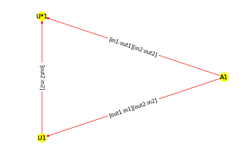
One difference (compared to the Mathematica code) is in the input line 8, where the weight is explicitly specified, here as . If one wants to use symbolic number for the initial weight, it must be defined as described below using the symbols command. Figure 13 shows the visualization of the initial tensor network before taking average. In this figure, matrices are represented as yellow disks and red arrows carry information about how matrices are connected. For example, consider the arrow from “U*1” to “A1”. The information “[in1:out1][in2:out2]” shows that this is a double edge, where the first bracket come from the edge “e3” and the second the edge “e4”.
Next, the following code averages the input graph over the unitary group and visualize it.
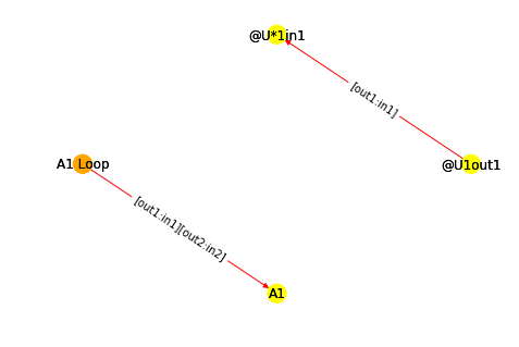
Note that in the input line 2, and are declared to be symbols explicitly. One can define other symbols in the same way. The algorithm calculates the average in input line 11 and outputs the result in the next line as shown in output line 1. The output is again a list, where the outer bracket are there in case the output is a sum of several tensor networks with corresponding weights. In this example, since we only have a pair of and , the average can be written as a single pair of a tensor network and a weight; the weight is now and the remainder of the output specifies the tensor network. The mark “@” corresponds to “dummy” in the Mathematica package. A visualization of the averaged tensor network is given in Figure 14. Loops are represented by orange disks. In this example, one orange disk is connected to the yellow disk labeled as “A1” by the red arrow with the information “[out1:in1][out2:in2]”. This means .
Appendix B Generating Weingarten functions
In this section, we provide a brief explanation of how the Python algorithm for generating Weingarten functions works, and show how to use it.
B.1. How the algorithm works
The formula for Weingarten functions (9) consists of two ingredients: characters of symmetric groups and Schur polynomials (i.e., characters of the unitary group) evaluated at the identity. Computation of the latter is straightforward based on the formula (10). The calculation of the former is rather complicated. We use the Murnaghan–Nakayama rule [Mur71, Nak41a, Nak41b]. There are recursive and non-recursive versions, and we choose to use a recursive one because it uses only Young diagrams, while the non-recursive ones requires manipulation of Young Tableaux. We refer to [Ber04] for a more detailed analysis of the problem of computing character tables of symmetric groups.
To make our paper self-contained, let us explain this recursive formula. The character table of the symmetric group is a square table, with entries indexed by two ordered partitions of . Here denotes a Young diagram specifying an irreducible representation, and is the character evaluated for any permutation with cycle type . A border strip is a connected set of boxes contained in a Young diagram. Now, fix and and take the Young diagram of the form and find all border strips within , denoted by , such that
- (1)
- (2)
removing from the Young diagram yields another Young diagram
- (3)
does not contain square.
We call any such border strip valid. From the second condition above it follows that the boxes of a valid border strip occupy the right-hand-side of each row of the Young diagram.
Let us consider some examples. Suppose . One can find two valid border strips of size (Figure 15) but none of size (Figure 16).
Then, calculate the height of each border strip , which is defined as
| (31) |
(In the notation introduced in Figure 15, the number of rows is the number of non-zero entries of .) The quantity then is given by the recursive formula
| (32) |
where the sum is over all valid border strips for the diagram . Here the expression refers to the Young diagram obtained by removing the boxes of from .
Let us illustrate this using the example of the diagram considered above. One can compute for example
| (33) |
where the sume was taken over the valid border strips and . By contrast,
| (34) |
because there is no border strip of size which can be removed from the Young diagram of .
Successive application of the recursive rule (32) leads to a linear combination of and , which are both defined to be . However, our program uses the rule (32) just once, and computes the character table of based on all the character tables of . This is why if one computes Weingarten functions for , the program automatically generates the character tables of .
B.2. How to use the Python RTNI package for generating Weingarten functions
One can generate Weingarten functions using the Python package. Example code is given here:
where is the size of the symmetric group. The output gives the Weingarten function for dimension (i.e., for the unitary group on ) as a list of pairs where (an ordered partition of ) is the cycle type and is any permutation with cycle type .
By choosing ’yes’ or ’no’, one can specify if the algorithm displays the result and if it should be recorded as ”functions” in the folder ”Weingarten”. In case the folder is missing, it is created automatically. In the example, and Weingarten functions for and are calculated in the output, being represented as a list. For example, the Weingarten function for the partition (cycle type) is .
Moreover, one can generate only the character tables of symmetric groups with the following code.
Here, is the size of the symmetric group, as before, and it is possible to choose if the algorithm shows the result or not. The result will be recorded automatically in the folder “SGC”, which is created in case it is missing. In this example, and each of the output tuples stands for an element of character table. For example, by using the notation in Section B.1, . All the above data is stored as “.pkl” files, which can be translated to text files by the program called “pkl2text”.