Singularities in Reissner-Nordström black holes

It is widely believed that long after black holes form their exterior geometry is described by the Kerr-Newman metric. The Kerr-Newman geometry naturally provides a mechanism for exterior perturbations to relax. Namely, perturbations are either absorbed by the black hole or radiated to infinity. Deep inside the black hole though, no such relaxation mechanism exists and the geometry depends on initial conditions.

While the geometry inside the black hole is not unique, it is natural to ask whether there are any universal features, such as the structure of singularities. Consider a black hole produced via gravitational collapse in asymptotically flat space, such as that shown in the Penrose diagram in Fig. 1. The collapsing body – the blue shaded region – results in an event horizon (EH) forming. In accord with Price’s Law [1, 2], collapse also results in an influx of radiation through the EH which decays with an inverse power $v^{-p}$ of advanced time $v$. Penrose reasoned more than 50 years ago [3] that infalling radiation will be infinitely blue shifted at the geometry’s Cauchy Horizon (CH), located at $v=\infty$, leading to a singularity there. For Reissner-Nordström (RN) black holes it was subsequently argued by Poisson and Israel [4, 5] that curvature scalars blow up like $e^{2\kappa v}$, where $\kappa$ is the surface gravity of the inner horizon of the associated RN solution, leading to a null singularity on the CH. Numerous studies [6, 7, 8, 4, 5, 9, 10, 11, 12, 13, 14, 15, 16, 17, 18, 19, 20] suggest that the presence of a null singularity at the CH is a generic feature of black hole interiors ¹¹ 1 A notable exception are near-extremal black holes in de Sitter spacetime [21]..

For small spherically symmetric perturbations of two-sided black holes, the null singularity on the CH can be the only singularity [22]. However, with large spherically symmetric perturbations, numerical simulations indicate that, in addition to a singular CH, a space-like singularity forms at areal radius $r=0$ [11, 12]. Likewise, for spherically symmetric one-side black holes, which form from gravitational collapse, numerical simulations also indicate the formation of a spacelike singularity at $r=0$ and a singular CH [13]. This means the singular structure of the spacetime is that shown in Fig. 1.

In this paper we focus primarily on one-side black holes (although we will discuss generalizations of our analysis to two-sided black holes in Sec. 5). We argue that the formation of a central spacelike singularity is inevitable in the collapse of a spherically symmetric charged scalar field in asymptotically flat spacetime. Our analysis employs three key assumptions. Firstly, we assume Price’s Law applies, meaning there is an influx of scalar radiation through the horizon which decays like $v^{-p}$ for some power $p$ which is sufficiently large such that the mass $M(v)$ and charge $Q(v)$ of the black hole approach constants $M(\infty)$ and $Q(\infty)$ as $v\to\infty$. The infalling radiation (which is left-moving in the Penrose diagram in Fig. 1) can scatter off the gravitational field and excite outgoing radiation (which is right-moving in the Penrose diagram). This, together with outgoing radiation emitted during collapse, means that the interior geometry of the black hole is filled with outgoing radiation.

Our second assumption is that the geometry at areal radius $r>r_{-}$ relaxes to the RN solution as $v\to\infty$. The radii $r_{\pm}$ are the inner $(-)$ and outer $(+)$ horizon radii of the RN solution with mass $M(\infty)$ and charge $Q(\infty)$ ²² 2 Recall that the surface $r=r_{-}$ is null for the RN solution. This need not be the case out of equilibrium. Indeed, prior to collapse the surface $r=r_{-}$ is time-like. Our analysis below implies that $r=r_{-}$ is spacelike at late times. ,

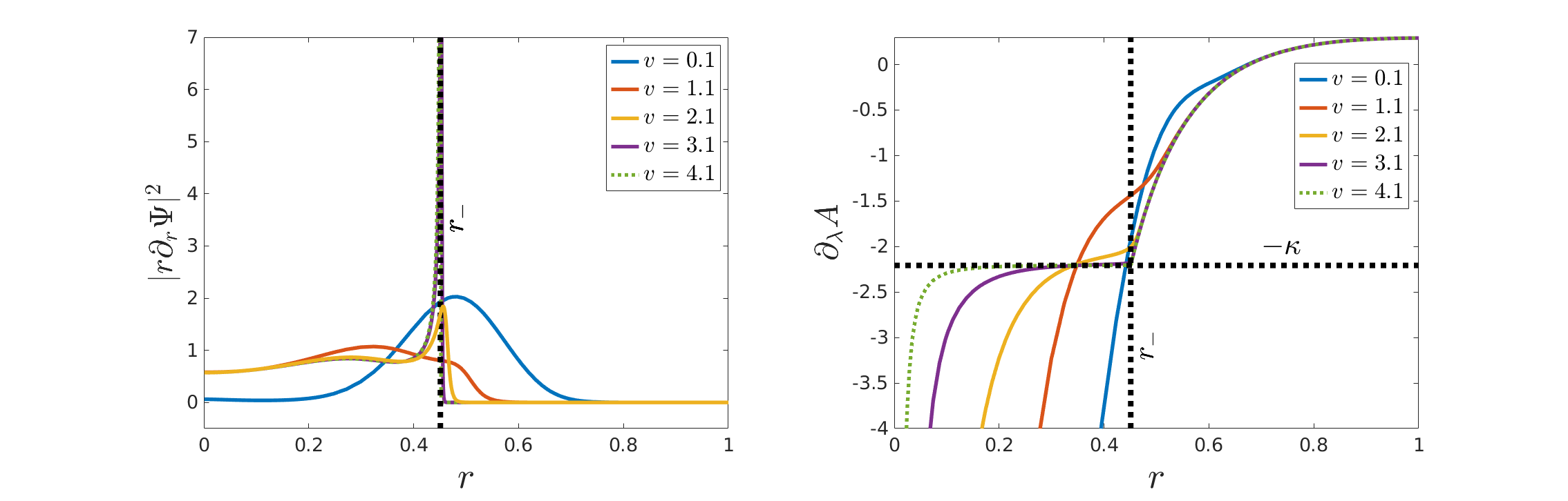
Why is it reasonable to assume the geometry at $r>r_{-}$ relaxes to the RN solution? In the RN geometry, all light rays at $r<r_{+}$, propagate to $r\leq r_{-}$ as $v\to\infty$. Therefore, the RN geometry naturally provides a mechanism for perturbations at $r>r_{-}$ to relax. To illustrate this further, in A we present a numerically generated solution to the equations of motion, Eqs. (6) below.

Our third assumption is that at any fixed time $v$, the geometry at $r>0$ contains no singularities. This assumption means the equations of motion can be integrated in all the way to $r>0$ without running into a singularity. We note, however, that this assumption is inconsistent with the weakly perturbed two-sided black holes studied in [22], where at finite time $v$, the outgoing branch of the singular CH lies at $r\approx r_{-}$. However, for one-sided black holes, numerical simulations indicate no singularities at $r>0$ at finite $v$ [13]. Additionally, our numerical simulations in the Appendix also show no signs of singularities at $r>0$ at finite $v$.

The assumption that the geometry at $r>r_{-}$ relaxes to the RN solution has profound consequences for late-time infalling observers passing through $r_{-}$. Firstly, as $v\to\infty$ outgoing radiation inside the black hole must be localized to a ball whose surface approaches $r_{-}$. This follows from the fact that in the RN geometry, all outgoing light rays between $r_{-}<r<r_{+}$ approach $r_{-}$ as $v\to\infty$. Moreover, from the perspective of infalling observers, the outgoing radiation appears blue shifted by a factor of $e^{\kappa v}$. This means that late-time infalling observers encounter an effective “shock” at $r=r_{-}$ [23, 24, 25, 26], where there is a searing ball of blue shifted radiation. In particular, upon passing through $r_{-}$, infalling observers will measure a Riemann tensor of order $e^{2\kappa v}$ and therefore experience exponentially large gravitational and tidal forces. Via Raychaudhuri’s equation, the ball of outgoing radiation focuses infalling null light rays from $r=r_{-}$ to $r=0$ over an affine parameter interval [23]

The scaling (2) has been verified numerically for spherically symmetric charged black holes [24] and for rotating black holes [25].

The exponential focusing of infalling geodesics suggests that at late times there exists an expansion parameter $\epsilon\equiv e^{-\kappa v}\ll 1$ in terms of which the equations of motion can be solved perturbatively in the region $r<r_{-}$. This can be made explicit by employing the affine parameter $\lambda$ of infalling null geodesics as a radial coordinate. With spherical symmetry the metric takes the form

where $\{\theta,\phi\}$ are polar and azimuthal angles respectively. Both $A$ and the areal coordinate $r$ depend on $v$ and $\lambda$. In this coordinate system curves with $dv=0$ are radial infalling null geodesics affinely parameterized by $\lambda$. Shocks at $r=r_{-}$ then imply derivatives w.r.t. $\lambda$ must diverge like $e^{\kappa v}$ in the region $r<r_{-}$. This means that inside $r_{-}$, the equations of motion can be expanded in powers of $\lambda$ derivatives (i.e. a derivative expansion). This is simply an expansion in powers of $\epsilon$, which is exponentially small as $v\to\infty$.

With the metric ansatz (3), initial data is naturally specified on some $v=v_{o}$ null surface. We consider the limit where $v_{o}$ is arbitrarily large. At $v>v_{o}$ we restrict our attention to the region inside two outgoing null surfaces $\mathcal{M}$ and $\mathcal{F}$, as depicted in Fig. 2. On $\mathcal{M}$ we impose the boundary condition that there is an influx of scalar radiation decaying like $v^{-p}$. In the shaded region between $\mathcal{M}$ and $\mathcal{F}$ we solve the equations of motion with a derivative expansion in $\lambda$. Why have we bothered to introduce $\mathcal{F}$? Why not just integrate deeper into the geometry? It turns out the surface $\mathcal{F}$ bounds the inner domain of validity of the derivative expansion: in the region enclosed by $\mathcal{F}$ the derivative expansion can break down. However, as depicted in Fig. 2, we find that $\mathcal{F}$ propagates inwards and intersects $r=0$ at a finite time $v$. In other words, the domain of dependence and validity of the derivative expansion initial value problem contains $r=0$ at late enough times.

We find that infalling radiation through $\mathcal{M}$ results in the Kretchmann scalar diverging like $e^{2\kappa v}$, consistent with previous demonstrations of a singular CH [6, 7, 8, 4, 5, 9, 10, 11, 12, 13, 14, 15, 16, 17, 18, 19]. Additionally, we find that infalling radiation results in a cloud of radiation forming near $r=0$. This cloud always results in a spacelike singularity forming at $r=0$ at late enough times, irrespective of initial conditions at $v=v_{o}$. In particular, the growing cloud of radiation results in the Kretchmann scalar diverging near $r=0$ like $r^{-2\alpha v}e^{2\kappa v}$ for some constant $\alpha>0$.

An outline of the rest of the paper is as follows. In Sec. 2 we write the equations of motion, employing the affine parameter $\lambda$ as a radial coordinate. In Sec. 3 we present the leading order equations of motion within the derivative expansion. In Sec. 4 we employ the leading order equations of motion to study the causal structure of singularities inside the black hole, and in Sec. 5 we present concluding remarks. In A, as an example, we present a numerical solution to the equation of motion.

We consider the dynamics of spherically symmetric charged black holes with a charged scalar field $\Psi$ and a gauge field $\mathcal{A}_{\mu}$. The equations of motion read

where $D_{\mu}$ is the covariant derivative, $\mathcal{D}_{\mu}=D_{\mu}-i\mathcal{A}_{\mu}$ is the gauge covariant derivative, and

are the scalar and electromagnetic stress tensors and electric current, respectively.

We work in the gauge $\mathcal{A}_{\lambda}=0$. With the metric ansatz (3), the components of the equation of motion (4) then read

where

is the electric field. The derivative operators ^′, $d_{+}$ and $\mathcal{D}_{+}$ are defined to be

The ^′ derivative is just the directional derivative along ingoing null geodesics whereas $d_{+}$ is the directional derivative along outgoing null geodesics. $\mathcal{D}_{+}$ is simply the gauge covariant version of $d_{+}$.

Eq. (6a) is an initial value constraint: if (6a) is satisfied at $v=v_{o}$, then the remaining equations guarantee it will remain satisfied at later times. Eqs. (6d) and (6g) are radial constraint equations: if (6d) and (6g) are satisfied at one value of $\lambda$, the remaining equations guarantee they will remain satisfied at all values of $\lambda$.

The equations of motion (6) constitute a nested system of linear ODEs. Given $\Psi$ at $v=v_{o}$ and boundary data on the outgoing null surface $\mathcal{M}$, shown in the Penrose diagram in Fig. 2, Eq. (6a) can be integrated in from $\mathcal{M}$ to find $r$. Next, given $\Psi$ and $r$, Eq. (6f) can be integrated in from $\mathcal{M}$ to find $\mathcal{A}_{0}$. With $\Psi$, $r$ and $\mathcal{A}_{0}$ known, Eq. (6b) can be integrated in from $\mathcal{M}$ to find $d_{+}r$. With $\Psi$, $r$, $\mathcal{A}_{0}$ and $d_{+}r$ known, Eq. (6e) can be integrated in to find $\mathcal{D}_{+}\Psi$. With $\Psi$, $r$, $\mathcal{A}_{0}$, $d_{+}r$ and $\mathcal{D}_{+}\Psi$ known, Eq. (6c) can be integrated in from $\mathcal{M}$ to find $A$. With $\Psi$, $\mathcal{A}_{0}$, $A$ and $\mathcal{D}_{+}\Psi$ known, we can compute $\partial_{v}\Psi$ and advance forward in time. Note the remaining equations, Eqs. (6d) and (6g), which are radial constraint equations, can be implemented as boundary conditions in the aforementioned radial integrations.

Following our arguments in the Introduction, in the region enclosed by the outgoing null surface $\mathcal{M}$ we shall solve the equations of motion (6) with a derivative expansion in $\lambda$. For pedagogical reasons we choose $\mathcal{M}$ to asymptote to $r=r_{-}$ as $v\to\infty$. However, it will turn out that the precise choice of $\mathcal{M}$ doesn’t matter for our analysis. One could equally well choose $\mathcal{M}$ to asymptote to some finite $r<r_{-}$.

The metric (3) is invariant under the residual diffeomorphism

where $\xi(v)$ is arbitrary. We exploit this residual diffeomorphism invariance to choose coordinates such that $\mathcal{M}$ lies at $\lambda=0$, with the spacetime enclosed by $\mathcal{M}$ lying at $\lambda<0$. Since $\mathcal{M}$ is null, this means

Additionally, the gauge choice $\mathcal{A}_{\lambda}=0$ enjoys the residual gauge freedom

where $\Lambda(v)$ is arbitrary. We exploit this residual gauge freedom to set

In order to account for rapid $\lambda$ dependence, we introduce a bookkeeping parameter $\epsilon$ and assume the following scaling relations for the directional derivatives along infalling and outgoing null geodesics,

We then study the equations of motion (6) in the $\epsilon\to 0$ limit. We shall see below that as advertised in the Introduction, $\epsilon=e^{-\kappa v}$. Hence the $\epsilon\to 0$ is just the $v\to\infty$ limit.

Why must we have $d_{+}=O(\epsilon^{0})?$ For any quantity $f$, the total $v$ derivative of $f$ along outgoing geodesics is $\frac{df}{dv}=d_{+}f$. Hence the scaling $d_{+}=O(\epsilon^{0})$ reflects the fact that quantities evaluated along outgoing null geodesics are not rapidly varying in $v$. The scalings (13) and Gauss’ law (6f) also imply $E=O(\epsilon^{0})$. Eq. (7) and the boundary condition (12) then imply

Likewise, the scaling relations (13) and the Einstein equation (6c) imply $A^{\prime\prime}=O(1/\epsilon)$. Together with the boundary condition (10), this means

Further boundary conditions are needed on $\mathcal{M}$. Firstly, we assume the influx of scalar radiation through $\mathcal{M}$ is a power law in accord with Price’s Law:

We leave $p$ arbitrary. Second, we fix a Neumann boundary condition on $A$. The scaling $A^{\prime}=O(\epsilon^{0})$ implies $\partial_{r}(A^{\prime})=O(\epsilon^{0})$. Hence it is reasonable to assume $A^{\prime}$ remains continuous in $r$ across $r_{-}$ as $\epsilon\to 0$, or equivalently as $v\to\infty$. We note this assumption is consistent with the numerical simulation presented in A. Additionally, we note this assumption is also constant with numerical solutions of the interior of rotating black holes [25]. With our assumption that the geometry at $r>r_{-}$ relaxes to the RN solution as $v\to\infty$, this means $A^{\prime}|_{\lambda=0}$ must approach its RN limit,

with $\kappa$ the surface gravity of the associated Reissner-Nordström inner horizon,

In the $\epsilon\to 0$ limit, Eqs. (6b)–(6e) and (6g) read

The remaining equations of motion (6a) and (6f) do not change in the $\epsilon\to 0$ limit.

Eq. (19a) can be integrated to yield

The constant of integration $\zeta(v)$ can be determined from the radial constraint equation (19c). Consider this equation evaluated on $\mathcal{M}$. Since $d_{+}$ is the directional derivative along outgoing null geodesics, Eq. (19c) can be rewritten on $\mathcal{M}$ as an ODE for $d_{+}r$,

where we have employed (17) to eliminate $A^{\prime}$. Employing Price’s law (16), in the $v\to\infty$ limit this equation is solved by (20) with

We emphasize that $d_{+}r<0$. This means there is no inner apparent horizon inside $\mathcal{M}$, for at an apparent horizon $d_{+}r=0$. Since $d_{+}r$ is the directional derivative of $r$ along outgoing null geodesics, Eqs. (20) and (22) yield the outgoing geodesic equation

Eq. (23) can be integrated to yield

It follows that geodesics with $r\leq r_{\rm c}$ end at $r=0$ whereas those with $r>r_{\rm c}$ end on the CH at finite values of $r$. This is consistent with the Penrose diagrams in Figs. 1 and 2. The critical radius $r_{\rm c}$ is given by

The remaining equations of motion (19b) and (19d) cannot be solved analytically without further approximations. In Sec. 3.1 we shall solve these equations near $\mathcal{M}$, where infalling radiation can be treated perturbatively, and establish the self-consistency condition that $\lambda$ derivatives indeed blow up like $e^{\kappa v}$. In Sec. 3.2 we shall show that near $r=0$, $\lambda$ derivatives blow up like $r^{-\alpha v}e^{\kappa v}$ where $\alpha>0$ is some constant. In Sec. 3.3 we discuss the domain of validity of the derivative expansion.

We now explore the consequences of the derivative expansion on the structure of singularities inside $\mathcal{M}$. First we will study the singularity on the Cauchy horizon at $v=\infty$. Using the equations of motion (6) to eliminate second order derivatives, without approximation the Kretschmann scalar $K\equiv R^{\mu\nu\alpha\beta}R_{\mu\nu\alpha\beta}$ reads

From the scaling relations (38) and (39) we see that the dominant terms in $K$ are the four in the first line. These all blow up like $e^{2\kappa v}$ as $v\to\infty$.

Let us first focus on the region near $\mathcal{M}$, where we can employ the solutions (26) for outgoing radiation. Without infalling radiation $K$ is regular near $\mathcal{M}$. However, due to the fact that $\lambda$ derivatives blow up exponentially like $e^{\kappa v}$, a tiny amount of infalling radiation leads to $K$ growing exponentially. Accounting for infalling radiation by employing (20), (22) and Price’s law (16) to determine $d_{+}r$ and $\mathcal{D}_{+}\Psi$, we see that the most singular terms in $K$ are the first two, which scale like

The physical origin of the exponential growth (43) is easy to understand. Consider for the sake of example two scalar wavepackets of wavelength $L_{+}$ and $L_{-}$ and amplitude $a_{+}$ and $a_{-}$. When the wavepackets pass through each other the Kretchmann scalar will scale like $(a_{+}/L_{+})^{2}(a_{-}/L_{-})^{2}$. In the limit where either $L_{\pm}\to 0$, the crossing fluxes of radiation will result in the Kretchmann scalar diverging. Inside the black hole the solution (26) provides an outgoing flux of scalar radiation while the influx is provided via Price’s law, (16). The final ingredient is that from the perspective of infalling observers, the outgoing radiation appears blue shifted by $e^{\kappa v}$ (which manifests itself in our coordinate system as $\lambda$ derivatives growing like $e^{\kappa v}$) ⁴⁴ 4 From the perspective of outgoing observers, ingoing radiation appears blue shifted by $e^{\kappa v}$.. This means that the crossing fluxes must result in a scalar curvature singularity on the CH which diverges like (43).

It is interesting to compare (43) to the contribution to the curvature from mass inflation [4, 5]. The mass function $m\sim r^{\prime}d_{+}r$ and hence, via the second term in (42), contributes to $K$ a term $\sim m^{2}$. From (20), (22) and (26) we see that $m^{2}\sim e^{2\kappa v}v^{-4p}$. Hence the contribution to the curvature from mass inflation is suppressed relative to that of the crossing fluxes by a factor of $v^{-2p}$. Similar results have been reported for rotating black holes in [17].

We now consider $K$ in the limit $r\to 0$. Using the scaling relations (38) and (39) we see that the $e^{2\kappa v}$ scaling in (43) must be enhanced to

as $r\to 0$. In other words, the exponential divergence near the Cauchy horizon becomes stronger when $r\to 0$.

We now turn to the nature of the singularity at $r=0$. From (44) we see that the divergence in $K$ near $r=0$ becomes stronger as $v$ increases. This is due to the buildup of scalar radiation near $r=0$ from infalling radiation. Moreover, it follows from the outgoing null geodesic solution (24) that geodesics at $r<r_{\rm c}$ with $r_{\rm c}\sim v^{1/2-p}$ must terminate at $r=0$ in a finite time $v$. This means that the singularity at $r=0$ must be spacelike.

In this paper we have introduced a novel approximation scheme valid in the interior of black holes which is simply a late-time expansion. Together with a set of assumptions, we have employed this scheme to show that decaying $1/v^{p}$ fluxes of radiation through the horizon necessitate the existence of a spacelike singularity at $r=0$. While we have focused on spherical symmetry, our analysis readily generalizes to geometries with no symmetry including that of rotating black holes. We shall report on this in a coming paper.

It is interesting that the structure of the singularity at $r=0$ is independent of the power $p$ of the infalling radiation. Indeed, the scalar energy density (36) just grows linearly with time $v$. This happens because the energy flux through $\mathcal{M}$ is time-independent. It turn out that the energy flux $\mathcal{S}$ through $\mathcal{M}$ is approximately time-independent so long as $|d_{+}\Psi|^{2}|_{\lambda=0}$ is slowly varying compared to $e^{-\kappa v}$. In particular, with this assumption Eqs. (20) and (21) yield $\zeta\sim|d_{+}\Psi|^{2}|_{\lambda=0}$ and Eq. (32) implies $\mathcal{S}\sim|d_{+}\Psi|^{2}|_{\lambda=0}/\zeta\sim 1$. This suggests our analysis can be generalized to de Sitter spacetime, where $|d_{+}\Psi|^{2}|_{\lambda=0}$ decays exponentially instead of with a power law. It would be interesting to study the scenarios found in [27, 21, 28]. We leave this for future work.

We conclude by discussing the generalization of our analysis to two-sided black holes. Two-sided black holes have both singular ingoing and outgoing branches of the CH, where the geometry effectively ends. For weakly perturbed two-sided black holes, the outgoing branch of the CH lies at $r_{\rm CH}(v)=r_{-}-\varepsilon$ where $\varepsilon\to 0$ characterizes the strength of the perturbations [22]. Therefore, when integrating the equations of motion (6) inwards along some $v={\rm const.}$ geodesic, one cannot integrate beyond $r=r_{\rm CH}$, since a singularity is encountered there. Correspondingly, our analysis of spacelike singularities, which takes place at $0\leq r<r_{\rm c}\ll r_{-}$, cannot be applied to weakly perturbed two-sided black holes. This is consistent with the results of Ref. [22], where it was demonstrated that weakly perturbed two-sided black holes only contain null singularities on the CH.

What happens when perturbations of two-sided black holes are large? With large perturbations there is no reason to expect $r_{\rm CH}(v)\approx r_{-}$. Indeed, numerical simulations of two-sided black holes with large perturbations indicate the CH contracts to $r=0$, at which point it meets a spacelike singularity [11, 12]. If at late times $r_{\rm CH}(v)\ll r_{\rm c}(v)$, then our analysis in this paper should apply. Namely, Price Law tails result in a growing cloud of scalar radiation forming at $r\lesssim r_{\rm c}$, which itself necessitates the existence of a spacelike singularity at late enough times with the curvature near $r=0$ growing like (44). We shall report on numerical simulations of such a scenario in an upcoming paper.

This work is supported by the Black Hole Initiative at Harvard University, which is funded by a grant from the John Templeton Foundation. EC is also supported by grant CU 338/1-1 from the Deutsche Forschungsgemeinschaft. We thank Amos Ori and Jordan Keller for many helpful conversations during the preparation of this paper.

References

- [1] R. H. Price, “Nonspherical perturbations of relativistic gravitational collapse. 1. Scalar and gravitational perturbations,” Phys. Rev. D5 (1972) 2419–2438.
- [2] R. H. Price, “Nonspherical Perturbations of Relativistic Gravitational Collapse. II. Integer-Spin, Zero-Rest-Mass Fields,” Phys. Rev. D5 (1972) 2439–2454.
- [3] R. Penrose, “Structure of space-time,”.
- [4] E. Poisson and W. Israel, “Inner-horizon instability and mass inflation in black holes,” Phys. Rev. Lett. 63 (1989) 1663–1666.
- [5] E. Poisson and W. Israel, “Internal structure of black holes,”Phys. Rev. D 41 (Mar, 1990) 1796–1809. https://link.aps.org/doi/10.1103/PhysRevD.41.1796.
- [6] M. Simpson and R. Penrose, “Internal instability in a Reissner-Nordstrom black hole,” Int. J. Theor. Phys. 7 (1973) 183–197.
- [7] W. A. Hiscock, “Evolution of the interior of a charged black hole,” Physics Letters A 83 (1981) no. 3, 110 – 112. http://www.sciencedirect.com/science/article/pii/0375960181905089.
- [8] Y. Gürsel, I. D. Novikov, V. D. Sandberg, and A. A. Starobinsky, “Final state of the evolution of the interior of a charged black hole,”Phys. Rev. D 20 (Sep, 1979) 1260–1270. https://link.aps.org/doi/10.1103/PhysRevD.20.1260.
- [9] A. Ori, “Inner structure of a charged black hole: An exact mass-inflation solution,”Phys. Rev. Lett. 67 (Aug, 1991) 789–792. https://link.aps.org/doi/10.1103/PhysRevLett.67.789.
- [10] M. L. Gnedin and N. Y. Gnedin, “Destruction of the cauchy horizon in the reissner-nordstrom black hole,” Classical and Quantum Gravity 10 (1993) no. 6, 1083. http://stacks.iop.org/0264-9381/10/i=6/a=006.
- [11] P. R. Brady and J. D. Smith, “Black hole singularities: A Numerical approach,” Phys. Rev. Lett. 75 (1995) 1256–1259, arXiv:gr-qc/9506067 [gr-qc].
- [12] L. M. Burko, “Structure of the black hole’s Cauchy horizon singularity,” Phys. Rev. Lett. 79 (1997) 4958–4961, arXiv:gr-qc/9710112 [gr-qc].
- [13] S. Hod and T. Piran, “Mass inflation in dynamical gravitational collapse of a charged scalar field,” Phys. Rev. Lett. 81 (1998) 1554–1557, arXiv:gr-qc/9803004 [gr-qc].
- [14] L. M. Burko and A. Ori, “Analytic study of the null singularity inside spherical charged black holes,” Phys. Rev. D57 (1998) 7084–7088, arXiv:gr-qc/9711032 [gr-qc].
- [15] M. Dafermos, “Stability and instability of the cauchy horizon for the spherically symmetric einstein-maxwell-scalar field equations,” Annals of Mathematics 158 (2003) no. 3, 875–928. http://www.jstor.org/stable/3597235.
- [16] M. Dafermos and J. Luk, “The interior of dynamical vacuum black holes I: The -stability of the Kerr Cauchy horizon,” arXiv:1710.01722 [gr-qc].
- [17] A. Ori, “Oscillatory null singularity inside realistic spinning black holes,” Phys. Rev. Lett. 83 (1999) 5423–5426, arXiv:gr-qc/0103012 [gr-qc].
- [18] A. Ori, “Perturbative approach to the inner structure of a rotating black hole,”General Relativity and Gravitation 29 (Jun, 1997) 881–929. https://doi.org/10.1023/A:1018887317656.
- [19] L. M. Burko, G. Khanna, and A. Zenginoǧlu, “Cauchy-horizon singularity inside perturbed Kerr black holes,” Phys. Rev. D93 (2016) no. 4, 041501, arXiv:1601.05120 [gr-qc]. [Erratum: Phys. Rev.D96,no.12,129903(2017)].
- [20] O. J. C. Dias, F. C. Eperon, H. S. Reall, and J. E. Santos, “Strong cosmic censorship in de Sitter space,” Phys. Rev. D97 (2018) no. 10, 104060, arXiv:1801.09694 [gr-qc].
- [21] V. Cardoso, J. L. Costa, K. Destounis, P. Hintz, and A. Jansen, “Quasinormal modes and Strong Cosmic Censorship,” Phys. Rev. Lett. 120 (2018) no. 3, 031103, arXiv:1711.10502 [gr-qc].
- [22] M. Dafermos, “Black holes without spacelike singularities,” Commun. Math. Phys. 332 (2014) 729–757, arXiv:1201.1797 [gr-qc].
- [23] D. Marolf and A. Ori, “Outgoing gravitational shock-wave at the inner horizon: The late-time limit of black hole interiors,” Phys. Rev. D86 (2012) 124026, arXiv:1109.5139 [gr-qc].
- [24] E. Eilon and A. Ori, “Numerical study of the gravitational shock wave inside a spherical charged black hole,” Phys. Rev. D94 (2016) no. 10, 104060, arXiv:1610.04355 [gr-qc].
- [25] P. M. Chesler, E. Curiel, and R. Narayan, “Numerical evolution of shocks in the interior of Kerr black holes,” Phys. Rev. D99 (2019) no. 8, 084033, arXiv:1808.07502 [gr-qc].
- [26] L. M. Burko and G. Khanna, “The Marolf-Ori singularity inside fast spinning black holes,” arXiv:1901.03413 [gr-qc].
- [27] J. L. Costa, P. M. Girão, J. Natário, and J. D. Silva, “On the Occurrence of Mass Inflation for the Einstein–Maxwell-Scalar Field System with a Cosmological Constant and an Exponential Price Law,” Commun. Math. Phys. 361 (2018) no. 1, 289–341, arXiv:1707.08975 [gr-qc].
- [28] R. Luna, M. Zilhão, V. Cardoso, J. L. Costa, and J. Natário, “Strong Cosmic Censorship: the nonlinear story,” Phys. Rev. D99 (2019) no. 6, 064014, arXiv:1810.00886 [gr-qc].
- [29] T. Mädler and J. Winicour, “Bondi-Sachs Formalism,” Scholarpedia 11 (2016) 33528, arXiv:1609.01731 [gr-qc].
- [30] P. M. Chesler and L. G. Yaffe, “Numerical solution of gravitational dynamics in asymptotically anti-de Sitter spacetimes,” JHEP 07 (2014) 086, arXiv:1309.1439 [hep-th].