A Comprehensive Theory and Variational Framework for Anti-aliasing Sampling Patterns115Journal: TOGVolume: 0000DOI: 0000001.0000001_2CCS: Computing methodologies AntialiasingCCS: Computing methodologies RenderingCCS: Computing methodologies Image processing

Abstract.
In this paper, we provide a comprehensive theory of anti-aliasing sampling patterns that explains and revises known results, and show how patterns as predicted by the theory can be generated via a variational optimization framework. We start by deriving the exact spectral expression for expected error in reconstructing an image in terms of power spectra of sampling patterns, and analyzing how the shape of power spectra is related to anti-aliasing properties. Based on this analysis, we then formulate the problem of generating anti-aliasing sampling patterns as constrained variational optimization on power spectra. This allows us to not rely on any parametric form, and thus explore the whole space of realizable spectra. We show that the resulting optimized sampling patterns lead to reconstructions with less visible aliasing artifacts, while keeping low frequencies as clean as possible.
Keywords:
Sampling, anti-aliasing, stochastic point processes, image processing, rendering1. Introduction
Sampling patterns are fundamental for many applications in computer graphics such as imaging, rendering, geometry sampling, natural distribution modeling, among others. They are of particular importance for reconstructing images from samples. Most real-world or synthesized images are not band-limited, i.e. they contain frequencies higher than those that can be represented with a finite number of samples, inevitably leading to aliasing. The challenge is avoiding aliasing artifacts that show up as secondary structures that are not present in the original image, while having the lower frequency content cleanly reconstructed. An ideal anti-aliasing sampling pattern thus preserves lower frequencies by introducing minimal noise, and maps all higher frequencies that cannot be represented with the sample budget to incoherent noise, instead of visible artifacts [Dippé and Wold 1985; Cook 1986].
A family of patterns proposed to approximate these properties are blue noise patterns [Ulichney 1988]. A zone plate image sampled with such a pattern, and the 2D and 1D power spectrum of the corresponding sampling pattern are depicted in Figure 1, left. The goal of blue noise patterns is to keep as large as possible, while minimizing deviations from for higher frequencies, with the intuition that the former will ensure clean low frequencies while the latter will lead to minimal aliasing. However, a perfectly flat power spectrum with for is only possible for quite low values of , and in general only random sampling can have a constant spectrum of for all . Low values lead to noisy low frequency content for sampled images, as visible in the limited clean region in the upper left corner of the zone plate image in Figure 1, left.
Many techniques have been proposed to generate sampling patterns for a larger range of cleanly represented frequencies, while avoiding aliasing artifacts as much as possible. Initial efforts focused on designing algorithms that impose constraints on certain geometric properties of the sampling patterns, such as the classical dart throwing algorithm [Cook 1986] and its variations, where sampling points are randomly distributed with a minimum distance between each pair. More recent techniques assume provided spectra or related statistics, and optimize locations of sampling points such that the resulting distributions have the given statistics [Zhou et al. 2012; Öztireli and Gross 2012; Heck et al. 2013; Wachtel et al. 2014; Ahmed et al. 2015; Kailkhura et al. 2016a]. This approach provides generic algorithms that can generate sampling patterns with any given characteristics such as a power spectrum.
The challenge, however, is how to specify useful shapes for power spectra in the limited space of realizable spectra [Uche et al. 2006]. Recent works have focused on generating realizable spectra with certain properties beneficial for anti-aliasing [Heck et al. 2013; Kailkhura et al. 2016a]. These methods assume a parametric form for power spectra, and search in the parameter space to have the least energy in the low frequency region, and a flat high frequency region bounded from above. Such a sampling pattern generated by a state-of-the-art technique [Kailkhura et al. 2016a] is shown in Figure 1, middle. The is significantly larger than that of step blue noise (left), which manifests itself as a larger range of clean low frequencies in the reconstructed zone plate image. However, this comes at the cost of a flat peak in the power spectrum, introducing artifacts in the zone plate image for middle frequencies. In general, assuming a given parametric form limits power spectra, leading to sub-optimal anti-aliasing properties.
In this paper, we introduce a comprehensive theoretical framework for anti-aliasing that leads to a variational approach to compute power spectra with optimized characteristics with respect to their anti-aliasing properties. In order to formulate the corresponding optimization problem, we first prove an analytic form for the spectrum of expected error introduced by sampling in terms of the power spectrum of the function to be represented and that of the sampling pattern. Based on this formula for error, we show how existing patterns improve anti-aliasing, and provide new theoretical results and insights. These are then translated into constraints and energies for formulating a constrained variational optimization on power spectra of point patterns. We show that careful selection of constraints and energies to minimize leads to sampling patterns with improved anti-aliasing properties. A sampling pattern generated by the proposed technique is shown in Figure 1, right. We get the same and thus range of noise-free lower frequencies as for the result of Kailkhura et al. [Kailkhura et al. 2016a], while still mapping all higher frequencies to almost white noise, as can be seen in the zone plate test image. The resulting power spectrum arises from our formulation of the optimization, without explicitly specifying its form.
In summary, we have the following main contributions:
- •
A theory of anti-aliasing with exact expressions for expected error spectrum. This allows us to analyze desirable properties for power spectra of point patterns for anti-aliasing.
- •
A new formulation of the problem of generating realizable spectral or spatial characteristics of point patterns based on variational optimization. We study different measures for optimality of sampling patterns, and show that there is a very rich family of realizable characteristics with desirable properties.
- •
Sampling patterns optimized for anti-aliasing with practical improvements over state-of-the-art patterns.
2. Related Work
Aliasing is a fundamental problem when reconstructing or synthesizing images with samples, as the images are typically not band-limited and we always have a finite budget of samples. It is well-known that regular sampling leads to structured aliasing, which introduces visually distracting extra structures. A main observation is that by injecting randomness into point distributions while satisfying certain properties, structured artifacts can be replaced with noise that is potentially visually less distractive [Dippé and Wold 1985; Cook 1986]. With such random distributions, it is important that high frequencies that cannot be represented with the sample budget are mapped to as incoherent as possible noise, ideally white noise to avoid any extra patterns in the reconstructed image, while keeping the important low frequency content clean.
Such sampling patterns are typically called blue noise in computer graphics. Blue noise patterns are characterized by a low energy power spectrum for , and a flat spectrum with for [Yellott 1983; Mitchell 1991]. Many methods have been proposed to generate point patterns with power spectra that exhibit variations of such properties. Earlier methods propose algorithms that impose certain constraints on the generated random point distributions. Dart throwing [Cook 1986] (also known as simple sequential inhibition and random sequential adsorption [Illian et al. 2008]) generates distributions where points are randomly placed in space with the constraint that no two points are closer to each other than a certain distance. This algorithm and the resulting distributions have been widely used and extended in many ways in the last decades (e.g. [Dunbar and Humphreys 2006; Bridson 2007; Wei 2008; Wei 2010; Ebeida et al. 2012; Ebeida et al. 2014; Yuksel 2015; Kailkhura et al. 2016b]). Other works have investigated utilizing alternative algorithms for improved characteristics for certain applications [Kopf et al. 2006; Ostromoukhov 2007; Illian et al. 2008; Balzer et al. 2009; Schmaltz et al. 2010; Fattal 2011; Schlömer et al. 2011; Xu et al. 2011; Chen et al. 2012; de Goes et al. 2012; Jiang et al. 2015]. The resulting point distributions are then analyzed by computing characteristics such as power spectrum, or statistics from stochastic point processes [Mitchell 1987; Lagae and Dutré 2008; Öztireli and Gross 2012; Heck et al. 2013], to understand their utility in practice.
A main limitation of the mentioned works for point pattern generation, however, is that the algorithm dictates the characteristics of the generated point patterns. Instead, a recent body of works propose to generate point distributions with statistics matching given ones [Zhou et al. 2012; Öztireli and Gross 2012; Heck et al. 2013; Wachtel et al. 2014; Ahmed et al. 2015; Kailkhura et al. 2016a]. Once a statistic, such as power spectrum, is defined, these methods run a routine to place sampling points such that the final configuration leads to the desired form for the statistic. With this approach, Heck et al. [Heck et al. 2013] could generate point distributions with the step blue noise spectrum for the first time (Figure 1, left). However, they have also observed that such a form for the spectrum is only possible for quite low values of , leading to noisy lower frequencies for sampled images. In general, the sub-space of realizable power spectra is restricted, with the necessary conditions that both power spectrum and pair correlation function, which is related to power spectrum with a spectral transform, should be non-negative [Uche et al. 2006]. Hence, a fundamental challenge is defining realizable forms for power spectra with desirable properties.
This challenge has been addressed by defining parametric forms for power spectrum in recent works [Heck et al. 2013; Kailkhura et al. 2016a]. The idea is then to search over the free parameters to get realizable power spectra with anti-aliasing properties. Heck et al. [Heck et al. 2013] define the single-peak blue noise, where a Gaussian is placed at around to trade off energy for against the maximum value of the power spectrum. The standard deviation, and magnitude of the Gaussian can then be altered to get realizable power spectra. Kailkhura et al. [Kailkhura et al. 2016a] have recently proposed a new parametrized family, stair blue noise, where the peak is replaced with a raised flat region of a certain width starting at , as in Figure 1, middle. The free parameters in this case are , and the width and height of the raised flat region. By a guided search over these parameters, spectra with a lower than single-peak blue noise can be obtained. However, for both methods, due to the assumed parametric forms, the families of power spectra considered are rather limited, and the exact effect of the parameters on aliasing is not clear.
In contrast, we do not assume any particular form for power spectra and instead formulate the problem of generating desirable and realizable spectra as constraint optimization with a variational formulation. This formulation rests on a theoretical analysis of properties of power spectra for anti-aliasing. Such an analysis has not been possible before due to the lack of an exact relation between error and power spectra of point patterns. After deriving this relation, we revise common properties of desirable power spectra. By formulating such anti-aliasing specific properties in addition to realizability conditions as constraints and energies, we then get diverse families of power spectra by variational optimization. This framework thus allows us to obtain optimal point patterns with respect to the imposed properties, e.g. for a given and perfectly zero energy for , we can get the minimum possible , up to numerical accuracy. The resulting point patterns lead to image reconstructions with less artifacts for high frequencies, and cleaner low frequency content.
3. Background and Preliminaries
We utilize the theory of stochastic point processes [Møller and Waagepetersen 2004; Illian et al. 2008] to understand anti-aliasing properties of point patterns. Stochastic point processes provide a principled approach for analyzing point patterns [Møller and Waagepetersen 2004; Illian et al. 2008]. A point process is defined as the generating process for multiple point distributions sharing certain characteristics. Hence, each distribution can be considered as a realization of an underlying point process (we use the term point pattern for families of point distributions sharing characteristics ).
We can explain a point process with joint probabilities of having points at certain locations in space. Such probabilities are expressed in terms of product densities. For our application of point patterns with optimal power spectra for anti-aliasing, it is sufficient to consider first and second order product densities, as they uniquely determine the power spectrum of a point process. First order product density is given by , where is the probability of having a point generated by the point process in the set of infinitesimal volume, and intuitively measures expected number of points around , i.e. local density. Similarly, second order product density is defined in terms of the joint probability of having points and in the sets and simultaneously, . It describes how points are arranged in space, and is fundamentally related to the power spectrum of .
As in previous works [Dippé and Wold 1985; Heck et al. 2013; Kailkhura et al. 2016a] on anti-aliasing, we will assume that no information is given on the function to be represented, and hence consider unadaptive point patterns. These patterns are generated by stationary and isotropic point processes, where the characteristics of the generated point distributions are translation invariant, or translation and rotation invariant, respectively [Öztireli and Gross 2012]. For both cases, reduces to a constant number, , which measures the expected number of points in any given volume, , where denotes expectation over different distributions generated by the point process , is the random number of points that fall into the set , and is its volume. For stationary point processes, second order product density becomes a function of the difference vector between point locations , which can be expressed in terms of the normalized pair correlation function (PCF) as . For isotropic point processes, PCF further simplifies and becomes a function of the distance between point locations . Below we will first consider stationary point processes and the associated derivations, which we will specialize to isotropic processes in the next sections.
PCF as a Distribution
The intuition behind PCF is that it can be estimated as a probability distribution of difference vectors (for stationary point processes), or distances (for isotropic point processes) between points. This is possible due to the fundamental Campbell’s theorem [Illian et al. 2008] that relates sums of functions at sample points to integrals of those functions. For simplicity of the expressions, we assume a toroidal domain with unit volume as the sampled domain (e.g. the image plane). Utilizing Campbell’s theorem, it is possible to derive the following expression for PCF of stationary processes (Appendix A)
| (1) |
where is the Dirac delta, and we defined , . Note that the ’s are from a particular distribution generated by the point process , and the expectation is over all such distributions. This expression clearly shows that PCF is simply a normalized distribution of difference vectors .
Power Spectrum and PCF
Power spectrum of a point process is defined in terms of the Fourier transform of the function as follows [Heck et al. 2013]
| (2) |
with denoting complex conjugate. Power spectrum thus lacks the phase of the Fourier transform and hence is translation invariant, only depending on the difference vectors . Equations 1 and 2 suggest that and are related by a Fourier transform. Indeed, denoting the Fourier transform of with , it is possible to derive the following relation between them (Appendix B)
| (3) |
In order to state properties of power spectra for anti-aliasing, we will work with a slightly modified form of Equation 3, where we rewrite the relation between and in terms a function we define, and its Fourier transform , as follows
| (4) |
Conditions for Realizable Power Spectra
Power spectrum is non-negative by definition (Equation 2), and this is also true for PCF as a distribution of difference vectors (Equation 1). Hence, two necessary conditions for a valid power spectrum of a point process are
| (5) |
It is still an open question whether these are also sufficient conditions, but no counterexamples have been shown in statistics and physics (e.g. [Torquato and Stillinger 2002]), and these conditions have been successfully used to generate realizable power spectra in previous works [Heck et al. 2013; Kailkhura et al. 2016a].
Error in Sampling a Function
Sampling a function with a point distribution generated by a point process can be written as in the spatial domain, or as in the frequency domain, where is the Fourier transform of , and denotes convolution. This sampled representation introduces an error. In order to analyze magnitude and distribution of error, the expected power spectrum of error needs to be computed [Dippé and Wold 1985; Heck et al. 2013]
| (6) |
where denotes magnitude of a complex number, and the sampled representation is divided by to normalize the energy of the sampled function [Heck et al. 2013], or equivalently to have an unbiased estimator since (by applying Equation 20 in Appendix A).
We need to relate the error to in order to derive desired properties for this statistic , which we elaborate on in the next section.
4. Theoretical Analysis of Sampling Error
The error spectrum provides how much error we get at each frequency. In general, we need to have as low as possible at each , and especially for low . For anti-aliasing, we need to additionally have an as uniform as possible to get incoherent noise instead of colored noise [Dippé and Wold 1985; Heck et al. 2013]. It is, however, not clear how these are exactly related to the shape of the power spectrum of a sampling pattern. We need this relation to be able to formulate the constraints and energies for our variational formulation of optimized sampling patterns for anti-aliasing.
4.1. Spectra of Error and Sampling Patterns
So far, relating to has only been possible for a constant function [Dippé and Wold 1985], or upper bounds could be derived for a sinusoidal wave [Heck et al. 2013]. In this section, we show that it is possible to derive an exact relation between and for an arbitrary , by utilizing the theory of point processes. This leads to theoretical justifications of criteria used for in the literature, and to novel theoretical results and insights.
We start by expanding the expression for the error spectrum in Equation 6 (we drop for brevity)
| (7) | ||||
where gives the real part of a complex number. The critical part of the proof is deriving the forms of these expected values. We show in Appendix C that this can be achieved by starting from Campbell’s theorem (as defined in Appendix A). The final form of the power spectrum of error is then
| (8) |
Here, is the power spectrum of the function .
Remarks
This expression immediately reveals several interesting properties of error when sampling a function.
- •
The error is independent of the phase of . This is expected as the sampling patterns considered are translation invariant.
- •
It implies that error can decrease as for any function , as observed for a sinusoidal wave previously [Heck et al. 2013]. However, at the same time, the difference vectors become smaller for higher number of points, leading to a compression of the domain of (Equation 1), and hence an expansion of that of , as they are related via a Fourier transform. Thus, the final convergence rate depends on and .
- •
The only pattern that gives a constant spectrum is random sampling (Poisson point process) with . In this case, we get , which leads to equally noisy frequencies and hence perfectly incoherent white noise.
In practice, a function (e.g. image) sampled with an anti-aliasing point pattern is then resampled to a regular grid after low-pass filtering. This can be written as (dropping for brevity), where is a low-pass filter such as Gaussian, and the points in are regularly distributed on a grid of e.g. pixel centers. This resampled function has the Fourier transform with and the Fourier transforms of and , respectively. As is an impulse train, the result of this convolution is repeating the same function, assuming avoids any overlap between aliases. Thus, only the central part around zero frequency, cut out by the filter , is relevant. The expected error (Equation 6) then becomes
| (9) |
Hence, we can consider the low frequency region of implied by for most practical applications.
Relation to integration
In this work, we are interested in error when representing a function with samples. This is fundamentally different than the error introduced by numerically integrating a function by summing the sample values. However, we can think of the sampling, filtering, and resampling of an image as performing local integration around each pixel center. This becomes clear if we explicitly write the process to compute . First, we can write . Convolving this with , we get . Finally, evaluating it at each pixel center , we get . Normalized by , this can be considered as a numerical approximation of the integral (| is the volume of ). To understand aliasing, we need to analyze the distribution of these errors of integral estimates at all pixels. Indeed, we are interested in the spectrum of error that encodes this distribution. This is in contrast with analyzing error in a single integral estimate.
Equation 8 further reveals an interesting relation with integration error. The DC component of sampling error given by is exactly the variance of the numerical estimator for the integral [Pilleboue et al. 2015; Öztireli 2016]. For the stationary point processes we consider, bias vanishes and hence this variance is equal to the expected error of the numerical integral estimator [Öztireli 2016].
4.2. Analysis of Anti-aliasing Properties
The derived relation between and allows us to perform a theoretical analysis of error in terms of the characteristics of the power spectrum. There are established characteristics for the power spectra of anti-aliasing point patterns in the literature. These follow certain intuitions and have indeed been effective in practice. However, how such characteristics exactly affect aliasing, and how they can be improved, could not be analyzed since the relation between and was not known [Heck et al. 2013].
There are two considerations for the error: 1) it should be low, 2) it should be as constant as possible, leading to white noise. The latter ensures that additional visual structures will not appear due to colored noise. We want to analyze how and thus should be shaped to achieve such a spectral profile for noise. For brevity, in the rest of the paper, we set , ignoring the Dirac delta at zero that does not contribute to .
Low energy for low frequencies
A fundamental property of anti-aliasing patterns such as blue noise patterns is that there should be a low energy low frequency region [Mitchell 1991; Heck et al. 2013; Kailkhura et al. 2016a], i.e. should be low and ideally zero for . This property is meant to limit the amount of noise at lower frequencies. By expanding the convolution in Equation 8, it can be easily shown for step blue-noise (Figure 1, left) where for , and otherwise, that
| (10) | ||||
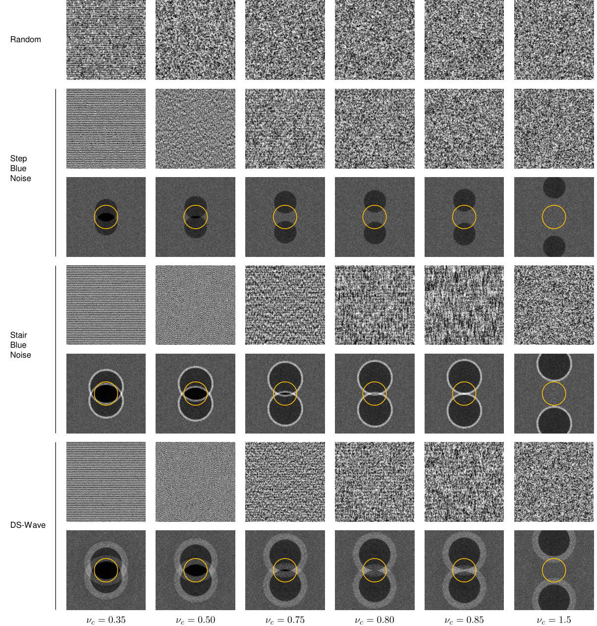
where is the -dimensional disk of radius , denotes the complement of a set, and and are the errors when using step blue noise, and random sampling, respectively. In particular, for a band-limited function with for , . However, in general, the difference between and may not be very large especially when the function has significant energy at higher frequencies. This can be seen in Figure 2, where we show examples of sampled images of a cosine wave of different frequencies , and the corresponding , for different sampling patterns. For high frequencies such as , the low frequency region (implied by the reconstruction kernel , marked with orange circles in the figure) of for step blue noise contains as much energy as for random sampling, leading to similar levels of error in the sampled images.
In practice, having a large is still very important even when sampling non-band-limited functions, due to the stationarity of the point patterns considered (Section 3). As the patterns are translation invariant, each local patch of the function is sampled with a point distribution of the same characteristics. Hence, the same analysis can be carried out for each patch. The visual quality especially for smoother patches, where noise is visually very distractive, will thus be improved significantly by using a step-like profile. This is illustrated in Figure 2 for , where stair blue noise and ds-wave sampling (a variation of our sampling patterns as we will discuss in Section 5) with a higher than step blue noise and random sampling, result in much cleaner image content.
Limiting the maximum of
Another fundamental property utilized in the literature is that the maximum of should be limited [Heck et al. 2013; Kailkhura et al. 2016a]. The intuition is that this will also limit the magnitude of and fluctuations in error. Indeed, we can easily show that
| (11) |
Hence, normalized by the total energy of , the error in this case is bounded by at every frequency .
This global maximum is also very important for limiting fluctuations in , i.e. avoiding colored noise. Example ’s where such maxima add up to generate significant fluctuations in error for low frequencies are shown in Figure 2, stair blue noise sampling with . In this case, for a constant , and hence the ratio of error to the total energy of the function is . In general for any function , this ratio can fluctuate between and at different frequencies, significantly disturbing the noise profile if the maximum is high. Such colored noise manifests itself as visually distinguishable secondary patterns in sampled images, as can be seen in the image reconstructions for stair blue noise with in the figure, instead of white noise without a clear structure.
Minimizing local maxima of
Due to the constraints on (Section 3), for point patterns with a larger , inevitably contains local maxima of decaying magnitude (as we will illustrate in Section 5). Apart from limiting , which determines the first maximum in , avoiding further local maxima is also beneficial, as these peaks can similarly sum up to cause further fluctuations in due to the convolution in Equation 8, albeit all smaller than as we illustrate in Figure 2. We will explore how we can shape the peaks such that we get an as small as possible global maximum and local maxima, while ensuring a certain , by translating these into energies and constraints in a variational optimization based formulation for in the next section.
5. Optimized Anti-aliasing Patterns
The characteristics for as elaborated on in the last section can be imposed in addition to the realizability conditions (Equation 5), to obtain optimal sampling patterns with respect to these criteria. In this section, we formulate the associated variational optimization problem. This will allow us to synthesize optimal distributions with respect to the considered characteristics with numerical solution methods.
5.1. Sampling as Constrained Variational Optimization
We start by making the effect of density on the problem explicit, and factor it out from the optimization. This can be achieved by working with normalized spatial and frequency coordinates. We start by defining . By the scaling property of Fourier transform, we can write . Substituting these into the expressions for and (Equation 4), we get , and (ignoring as before, as it does not contribute to ). Then, in normalized coordinates, we can write the conditions and as
| (12) |
Thus, the constraints become independent of the intensity of the point process. We will work with and in normalized coordinates unless stated otherwise, and set , and . Absolute spatial coordinates are thus given by multiplying the reported with , and absolute frequencies by multiplying the reported with .
Although the complete analysis in the rest of the paper can be carried out for stationary point processes in , we will consider the important case of image sampling with non-adaptive anti-aliasing distributions as in previous works [Dippé and Wold 1985; Heck et al. 2013; Kailkhura et al. 2016a]. This implies that the point processes considered are isotropic, generating rotation and translation invariant distributions. In this case, and thus is radially symmetric such that , , and all Fourier transforms in the definitions above turn into Hankel transforms . In particular, we have , or equivalently . The Hankel transform is defined for any dimensions. For our case of sampling the image plane, we use the Hankel transform for dimensions.
Hence, the problem becomes finding a 1D function with the above non-negativity constraints in Equation 12, and additional properties we impose. These properties can either be set as hard inequality constraints , or energies that we minimize for. We can thus formulate the following constrained variational minimization problem on , to find a realizable and desirable
| (13) |
5.2. Constraints and Energies for Anti-aliasing
By changing the energy functional and constraints , we can tune the properties of and thus . We summarize the properties shaped by the constraints and energies considered in Figure 3. These closely follow the criteria analyzed in Section 4, with a low energy low frequency region, bounded global maximum and local maxima.
Low Frequency Constraint
We start with the property that has small energy for for a given (we call this region as the low frequency region, and as the high frequency region). This can be imposed with a direct constraint of the form , for a limit . Similar terms have been used to quantify the energy in the low frequency region in previous works [Heck et al. 2013; Kailkhura et al. 2016a]. However, this does not limit the value of at a given frequency, and hence can grow very large, leading to severely high error at certain low frequencies, and hence significant fluctuations in the spectrum. An example spectrum generated with this integral constraint is shown in Figure 4, left. Instead, we propose to directly limit the spectrum for the low frequency region with
| (14) |
This ensures that error will be bounded at all low frequencies (Figure 4, right). Ideally, , and thus for . We will see in the next section that and hence noise for low frequencies can be traded off with aliasing at higher frequencies. For the analysis in this section, we assume .
Oscillation Energy
Another desired property of is that it should not have high global and local maxima. This can be imposed in several ways. Previous works [Heck et al. 2013] have considered measuring squared deviation of from , which can be written as the following energy
| (15) |
Minimizing this energy with the realizability constraints and the low frequency constraint above for different ’s, we get the spectra in Figure 5, top. We get a perfectly zero region for , and peaks of decaying magnitude for higher frequencies. This is a typically encountered profile for blue noise patterns, except for two recent works [Heck et al. 2013; Kailkhura et al. 2016a]. For , which is the theoretical limit for a step-noise profile, we get a perfect step shape. Larger leads to oscillations, with the magnitude of the first peak determining the global maximum of . As is increased, the maximum also gets larger.
Total Variation Energy
For and , will inevitably deviate from with one or more peaks, before it (possibly) converges to [Heck et al. 2013]. An alternative way of limiting the magnitudes of these peaks is to minimize total variation energy. This can be visualized as minimizing the length of the path traveled by a point when projected onto the -axis, as it moves along the curve from to . The resulting energy is given by
| (16) |
We show power spectra generated by minimizing this energy under the low frequency constraint and realizability conditions in Figure 5, bottom. The spectra now mostly contain raised rectangular regions instead of peaks, i.e. a decaying square wave. This is due to the sparse gradients introduced by total variation. Heights of rectangular regions, and thus the maxima of are smaller than when minimizing the oscillation energy above.
Smoothness Energy
We further experimented with smoothness energies, the Dirichlet energy , and Laplacian energy . We show the resulting spectra in Figure 6. The spectra in these cases are worse with higher peaks than with oscillation or total variation energy.
Maximum Constraint
Although total variation energy leads to peaks of smaller magnitude, it might still be possible to further reduce the global maximum of . The same is true for all energies. Having a small is an important factor to avoid colored noise and hence aliasing, as elaborated on in Section 4.2. To achieve a smaller , we limit the magnitude of deviations from with the following constraint
| (17) |
In practice, this constraint is equivalent to , as for all power spectra in previous works and in this work, the first peak has the largest , and at that peak (e.g. Figure 5). Of course, not all - combinations are realizable (we will elaborate more on this point in the next section). In order to define the range of possible for a given , we can find the minimum possible by an exhaustive search. We show this constraint imposed on the spectra for oscillation energy and total variation energy in Figure 7. For both energies, reducing comes at the cost of a larger number of oscillations, albeit all with smaller magnitudes, hence not leading to significant aliasing.
5.3. Optimized Sampling Patterns
The analysis above suggests that total variation energy leads to better profiles for power spectra, with lower global and local maxima. Without the maximum constraint (Equation 17), the maximum with oscillation energy is larger (Figure 7, left), while imposing the maximum constraint results in further peaks of higher magnitudes than those with total variation energy as in Figure 7, right (please see the supplementary material for more spectra with total variation and oscillation energies). Due to the flatter shape of the spectrum, noise is introduced for a larger range of unrepresentable high frequencies with total variation energy. However, such incoherent noise is preferred to colored noise caused by higher maxima in power spectra with oscillation energy. Hence, we focus on total variation (Equation 16) as the energy in this paper. Due to its shape resembling a decaying square wave, we call the resulting pattern as ds-wave sampling.
The use of the maximum constraint depends on the gain we obtain, i.e. how much lower the maximum of the power spectrum is with this constraint. We show estimated power spectra without () and with the maximum constraint for , and (the minimum possible ) in Figure 9. These are computed as the empirical power spectra of generated point distributions (we elaborate more on this in the next section). As we use total variation energy, we already get low maxima, hence see only a marginal improvement. In general, it is possible to tune depending on how critical this improvement is for the application, but this requires a search among different values, and some additional local maxima appear in the spectrum.
Recent works [Heck et al. 2013; Kailkhura et al. 2016a] explore minimizing maximum of power spectra for a given and . However, as they use pre-defined parametric families of functions, it is not possible to achieve the minimum possible maximum. By utilizing the proposed optimization framework, we can derive the minimal maximum (up to numerical accuracy). For fixed and , we try to optimize any of the above energies for various ’s, and take the minimum that leads to a feasible solution. The resulting space of feasible - pairs are shown in Figure 8 for and . Note that these results are general and independent of the form of the power spectrum. The minimum possible stays at for as expected, and becomes increasingly more sensitive to for large values. It is not possible to go beyond , as this is the of regular sampling. We also observe this in practice when we compute the feasible region. We can use the feasible region as a benchmark for how patterns perform for anti-aliasing.

As Figure 8, right, shows, increasing low frequency noise with significantly reduces , especially for high values of . We show power spectra obtained for and in Figure 9. Although the constraint is for , the optimizations result in for all . For higher ’s, power spectra get flatter, and thus zone plate images show reduced aliasing artifacts for high frequencies. This comes at the cost of higher levels of noise introduced into low frequencies, as visible in low frequency parts of the zone plate images. The generated point distributions reveal the source of this low frequency noise: they become increasingly more random for larger values of .
5.4. Implementation
We discretize the problem in Equation 13 with standard techniques from numerical analysis. As the function to optimize for is -dimensional, a simple discretization with regular sampling is used. The derivative operators are then discretized with finite differences, and integrals in the energies are approximated with the trapezoidal rule. Hankel transform is discretized with an accurate approximation based on the trapezoidal rule (e.g. [Cree and Bones 1993], Equation 6).
We experimented with various ranges and sampling rates for and . In all of our experiments, a sample spacing of was sufficient for accurate numerical results. In order to test the accuracy of the resulting spectra with this spacing, we take spectra with randomly chosen parameters (, and to avoid having many step-like spectra). We then compute the average root mean squared difference between each spectrum for a sample spacing of and , resulting in average difference. For , we sample the range , since well before , converges to (and hence converges to ) for all patterns in our experiments. The average absolute deviation of from for for random spectra is . The same, however, is not true for , which determines the PCF . For , we thus sample almost the full range of possible distances for the unit toroidal domain we consider, in absolute coordinates. Note, however, that in practice this is not strictly needed as we only require , and does not oscillate significantly beyond a limited range of ’s.
Hankel transform is a linear operator and hence all constraints, including the realizability conditions (Equation 12), are linear inequality constraints. The oscillation (Equation 15) and smoothness energies turn into quadratic forms when discretized. For these energies, the discrete problem thus becomes quadratic programming. Minimization with total variation energy (Equation 16) can be formulated as linear programming, using well-known results from optimization. Both problems are thus convex and easy to solve with any modern optimization package. We use built-in Matlab functions for optimization.
There are several techniques for synthesis of point patterns based on PCF or power spectrum [Zhou et al. 2012; Öztireli and Gross 2012; Heck et al. 2013; Wachtel et al. 2014; Ahmed et al. 2015; Kailkhura et al. 2016a]. We experimented with several of these approaches that focus on accuracy [Öztireli and Gross 2012; Heck et al. 2013; Kailkhura et al. 2016a], and got similar results. We hence use the PCF-based matching technique of Heck et al. [Heck et al. 2013] for all experiments in the paper and the supplementary material, due to the efficient implementation available. We use the default parameters for that algorithm, and the same discretization for PCF as we describe above.
6. Evaluation and Analysis
To evaluate the performance of our sampling patterns in practice, we analyze power spectra, and illustrate their anti-aliasing properties on sampled images (for more results, please see the supplementary material).
Evaluation
For estimating the power spectrum of a pattern, we generate point distributions with a matching spectrum, each with points. The empirical power spectra of these distributions, computed with Equation 2 and their radial averages, are averaged to generate all estimated 2D and 1D power spectra in this paper and the supplementary material. For other sampling patterns that start from a theoretical power spectrum (step blue noise, single-peak blue noise [Heck et al. 2013], and stair blue noise [Kailkhura et al. 2016a]), we use the same point distribution synthesis algorithm [Heck et al. 2013] with the same settings as in Section 5.4.
Unless stated otherwise, we use distributions with () points at sample per pixel (spp) for all test images except the zone plate images. We use the zone plate function (, ) as a benchmark test image, since it reveals aliasing at different frequencies without the masking effect due to local structures [Heck et al. 2013; Kailkhura et al. 2016a]. These images are sampled at spp (please see the supplementary material for zone plate images with spp). All images are reconstructed with a low-pass filter (we use the Gaussian filter) and resampled to a regular grid. This filter and others used in the literature retain some of the frequencies that cannot be represented with the pixel grid, but ensure a clear visualization of noise. In practice, we only noticed faint and distinct secondary rings for zone plate images when using more than samples per pixel due to this filtering, as visible e.g. in Figure 1.

Ds-wave and Stair Blue Noise
We analyze the properties of our ds-wave sampling and compare them to those of the state-of-the-art stair blue noise sampling [Kailkhura et al. 2016a] in Figure 10. For stair blue noise, at each , we find the minimum value for the maximum of the power spectrum with an exhaustive search over the parameters, as described by Kailkhura et al. [Kailkhura et al. 2016a]. Since stair blue noise has zero energy for the low frequency region, we set for all comparisons.
Figure 10, left shows that for all (the theoretical limit for step blue noise), ds-wave sampling has a lower than stair blue noise, with the difference getting larger for larger . Ds-wave sampling with achieves the optimal , by definition. But even without the maximum constraint (i.e. ), ds-wave sampling has very close to the optimum. Note that the maximum we could obtain for stair blue noise sampling for is , and thus we show the range . In Figure 10, right, we plot the spectra for , illustrating the significant difference between ds-wave and stair blue noise for both and . We show further theoretical, and estimated 2D and 1D spectra for lower ’s in Figure 11 (). For all cases, the theoretical spectra of ds-wave sampling can be realized reliably, with a lower maximum than stair blue noise, and almost no further oscillations. The difference is especially significant for higher values of . Please see the supplementary material for more examples of theoretical and estimated spectra.
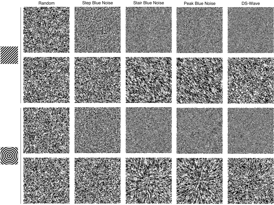
The practical utility of these results is illustrated in Figures 1 (, ), 2 (, ), and 12 (, ). In Figure 1, the zone plate image reveals frequencies that are mapped to colored noise and hence secondary patterns due to the high magnitude region for stair blue noise sampling. Ds-wave sampling maps such unrepresentable high frequency content to noise with a profile closer to that for step blue noise, while preserving the same , and thus noise levels for low frequency content, as stair blue noise. Although noise is introduced into a larger range of higher frequencies, this noise is much less objectionable than the patterns introduced by stair blue noise. We illustrate this further in Figures 2 and 12 for images with repeated structures of several frequencies. The cleaner reconstructions of repeated structures of lower frequencies (top rows) provided by stair blue noise sampling come at the expense of mapping repeated structures of frequencies higher than the representable frequency to colored noise. This manifests itself as secondary patterns and higher levels of noise in the sampled images (bottom rows). Ds-wave sampling leads to as white as possible noise for these cases, combining advantages of step and stair blue noise sampling.
Ds-wave and Other Patterns
We compare ds-wave sampling to further patterns commonly used for anti-aliasing in Figure 13. Dart throwing results in a relatively small and hence does not lead to objectionable aliasing artifacts. However, it also leads to low frequency noise in sampled images, as is apparent for the zone plate image. For a wider range of cleaner low frequencies for sampled images (i.e. a larger low frequency region in power spectrum), CCCVT centroids [Balzer et al. 2009] can be utilized. This results, however, in higher peak values, and thus more pronounced aliasing artifacts.
An even larger low frequency region is possible with single-peak blue noise sampling [Heck et al. 2013], as illustrated in Figure 13, middle. Note that single-peak blue noise is not exactly zero at low frequencies due to the introduced Gaussian at around the transition from low to high frequencies, while ds-wave sampling has zero energy in the low frequency region. We set such that both single-peak and ds-wave reach the first time at approximately the same . At this size of the low frequency region, the peak has a high value and aliasing becomes apparent as secondary patterns in the zone plate image in Figure 13, middle, and the sampled high frequency repeated stripe patterns (bottom rows) in Figure 12. Our ds-wave sampling at and has the same size of the low frequency region, but with a lower maximum, and hence leads to lower noise and aliasing, as visible in the same figures.
The maximum and hence aliasing artifacts can be further reduced by introducing low frequency noise. With , we get a slightly smaller than dart throwing, while still having cleaner and a larger range of low frequencies than dart throwing as shown in Figure 13.
Multiple Samples per Pixel
One way of reducing noise is increasing number of samples per pixel. However, if contains high peaks, for finite spp, there will always be secondary patterns due to aliasing when sampling image content of certain frequencies. To see this, we start by noting that the error after resampling to a regular grid is given by , as derived in Section 4.1. Increasing spp means we are keeping the same, and expanding (as it is related to with a Fourier transform, which compresses for larger number of points due to smaller distances among them, please see Section 3). If has peaks, they will thus be shifted to higher frequencies and be smoothed as a result of this expansion. If a sampled image has local structures of those frequencies, due to the convolution in the definition of , these peaks will then be shifted to lower frequencies that are captured by the filter . Hence, similar but smoothed artifacts in the form of visible secondary patterns will appear in the final reconstructed image.
This is illustrated in Figure 14 for the cosine function in Figure 2 with . We use spp for the top row, and spp for the bottom row. Note that as we always normalize frequencies by the number of sampling points, the absolute frequency shifts with the spp. For both cases, increasing spp does not help to reduce the visible secondary structures due to aliasing. In fact, higher spp might lead to perceptually more apparent secondary structures, e.g. for spp in Figure 14.
Artifacts on Rendered Images
We illustrate such aliasing artifacts for practical rendered scenes in Figure 15. For this figure, we sample each of the dimensions for the light transport, except the image plane, densely. Hence, the spp reported corresponds to the image plane samples. Computing each of those image plane samples is thus a costly operation involving a numerical integration for all other dimensions. We show a reference image first, then the result of stair blue noise on a smaller image with or spp on the left, and the corresponding result with ds-wave sampling on the right. Note that we intentionally did not resample the rendered small images with nearest neighbor sampling to illustrate that applying standard filters on the images with aliasing artifacts does not alleviate the aliasing artifacts due to colored noise. For certain scenes such as the top image, increasing the spp from to makes the aliasing artifacts more apparent. In general, we observed that ds-wave sampling makes the most difference for directional repeated structures as exemplified in the figure.
Running Time
The formulation of the optimization problems with linear and quadratic programming allows us to use efficient and robust solvers. For total variation energy (linear programming), it takes - minutes for the solver to converge on a PC with Intel(R) Xeon(R) CPU ES-2680 v3 @ GHz, with the running time increasing for larger . As this optimization is done once and offline, the main computational complexity comes from the point distribution generation procedure [Heck et al. 2013], which takes about one minute to converge for points.
7. Conclusions and Future Work
We presented a theoretical and practical framework for analyzing aliasing, and generating sampling patterns with optimized properties for anti-aliasing via formulating the problem of generating realizable spectra as variational optimization. The resulting patterns lead to practical improvements in reducing aliasing artifacts due to colored noise, and the proposed theoretical framework allows us to explore and revise optimality measures used for anti-aliasing. We see many interesting uses of this framework for future research, some of which we summarize below.
Sampling for Integration
Although we focused on anti-aliasing when reconstructing images in the scope of this paper, a very promising direction is to optimize power spectra for reducing error in numerical integration. Recent works [Öztireli 2016; Pilleboue et al. 2015] have proved that the dependence of error on power spectrum is given by , as we also discussed in Section 4.1. Minimizing this error will turn into a linear programming problem when formulated as variational optimization, similar to Equation 13. Once characteristics of integrands are determined, we can get specialized optimal spectra as well.
Adaptive Anti-aliasing Patterns
Similar to previous works, we considered non-adaptive anti-aliasing patterns, with no information on the actual image to be represented. Recent works [Roveri et al. 2017] show that sampling patterns with adaptive second order product densities can lead to significant accuracy improvements for image representation and processing. By combining our optimization framework with locally adaptive point distribution synthesis algorithms [Roveri et al. 2017], we can obtain optimal adaptive sampling patterns for image reconstruction.
Exploration of Second Order Characteristics
Previous works explore the space of valid second order characteristics either via analysis of available point patterns [Öztireli and Gross 2012], or parametrized families of power spectra [Heck et al. 2013; Kailkhura et al. 2016a]. Our framework can be used to explore this space without such constraints. As an example, we showed that optimal maximal values for power spectra for given ’s can be obtained (Figure 8). Similar results can be derived for other applications such as geometry sampling, physically-based simulations, or natural distributions.

Higher Dimensional Sampling
An interesting aspect of the optimization problem in Equation 13 is that it depends on the dimensionality due to the Hankel transform. We will thus get different spectra for different dimensions, as Hankel transform takes a different form for different dimensions. It will be interesting to explore optimal sampling patterns for higher dimensions, e.g. in the context of rendering where the integrands can be very high dimensional.

Synthesis of Point Patterns
Our approach essentially formulates point pattern generation as a two-step procedure, where we first optimize for a power spectrum, and then generate point distributions with that power spectrum. It is an ongoing research to synthesize point distributions with given statistics. Although the PCF based synthesis algorithm we use [Heck et al. 2013], and others we tested [Öztireli and Gross 2012; Kailkhura et al. 2016a] give very accurate results, all have a hard time to synthesize highly regular point sets (e.g. point distributions with , , and in the supplementary material), as also observed in earlier works [Öztireli and Gross 2012]. As the synthesis algorithms evolve, the proposed formulation can be tuned further for the particular synthesis algorithm considered. For example, for a PCF based matching algorithm, the runtime can be reduced by considering a limited range for the PCF, which is possible if PCF is constant outside that range. This can be explicitly imposed as a constraint in our framework.
Appendix A Derivation of PCF as a Distribution
Campbell’s theorem [Illian et al. 2008] gives sums of functions at sample points as integrals of those functions. For our case with the toroidal unit domain , we can write the theorem for first and second order product densities as
| (18) |
| (19) |
provided some technical conditions are satisfied for the point process and the function [Illian et al. 2008]. For stationary point processes, these simplify to
| (20) |
| (21) |
Substituting for in Equation 21, we get
| (22) | ||||
proving that can be estimated as the distribution of difference vectors.

Appendix B Relation between PCF and Power Spectrum
Appendix C Derivation of Error Spectrum
We start by rewriting the form of the error in Equation 7
| (26) |
As defined in Section 3, and thus its Fourier transform is . Plugging this into the Campbell’s theorem of first order (Equation 20) we get
| (27) |
The last term in Equation 26 thus becomes . Calculating the first term in Equation 26 is more involved due to the squared magnitude. We first expand this term with the definition of and utilizing properties of the Fourier transform
| (28) | ||||
where we used the notation for , and the equivalence . The expected value of the first term on the last line can be computed with Campbell’s theorem of first order (Equation 20) as . The second term involves a double sum, and the expected value can thus be computed by utilizing Equation 21 as
| (29) | ||||
with denoting the autocorrelation of , and we use the relation , and the multiplication theorem of Fourier transform. Substituting the expression for (Equation 4), this can also be written in terms of as . Summing the two terms in Equation 28, we thus get
| (30) |
Finally, we sum all the terms in Equation 26
| (31) | ||||
References
- [1]
- Ahmed et al. [2015] Abdalla G. M. Ahmed, Hui Huang, and Oliver Deussen. 2015. AA Patterns for Point Sets with Controlled Spectral Properties. ACM Trans. Graph. 34, 6, Article 212 (Oct. 2015), 8 pages.
- Balzer et al. [2009] Michael Balzer, Thomas Schlömer, and Oliver Deussen. 2009. Capacity-constrained Point Distributions: A Variant of Lloyd’s Method. ACM Trans. Graph. 28, 3, Article 86 (July 2009), 8 pages.
- Bridson [2007] Robert Bridson. 2007. Fast Poisson Disk Sampling in Arbitrary Dimensions. In ACM SIGGRAPH 2007 Sketches (SIGGRAPH ’07). ACM, New York, NY, USA, Article 22. DOI:https://doi.org/10.1145/1278780.1278807
- Chen et al. [2012] Zhonggui Chen, Zhan Yuan, Yi-King Choi, Ligang Liu, and Wenping Wang. 2012. Variational Blue Noise Sampling. IEEE Transactions on Visualization and Computer Graphics 18, 10 (Oct. 2012), 1784–1796. DOI:https://doi.org/10.1109/TVCG.2012.94
- Cook [1986] Robert L. Cook. 1986. Stochastic sampling in computer graphics. ACM Trans. Graph. 5, 1 (1986), 51–72.
- Cree and Bones [1993] M.J. Cree and P.J. Bones. 1993. Algorithms to numerically evaluate the Hankel transform. Computers & Mathematics with Applications 26, 1 (1993), 1 – 12. DOI:https://doi.org/10.1016/0898-1221(93)90081-6
- de Goes et al. [2012] Fernando de Goes, Katherine Breeden, Victor Ostromoukhov, and Mathieu Desbrun. 2012. Blue Noise Through Optimal Transport. ACM Trans. Graph. 31, 6, Article 171 (Nov. 2012), 11 pages.
- Dippé and Wold [1985] Mark A. Z. Dippé and Erling Henry Wold. 1985. Antialiasing Through Stochastic Sampling. SIGGRAPH Comput. Graph. 19, 3 (July 1985), 69–78. DOI:https://doi.org/10.1145/325165.325182
- Dunbar and Humphreys [2006] Daniel Dunbar and Greg Humphreys. 2006. A spatial data structure for fast Poisson-disk sample generation. ACM Trans. Graph. 25 (July 2006), 503–508. Issue 3.
- Ebeida et al. [2012] Mohamed S. Ebeida, Scott A. Mitchell, Anjul Patney, Andrew A. Davidson, and John D. Owens. 2012. A Simple Algorithm for Maximal Poisson-Disk Sampling in High Dimensions. Comput. Graph. Forum 31, 2pt4 (2012), 785–794.
- Ebeida et al. [2014] Mohamed S. Ebeida, Anjul Patney, Scott A. Mitchell, Keith R. Dalbey, Andrew A. Davidson, and John D. Owens. 2014. K-d Darts: Sampling by K-dimensional Flat Searches. ACM Trans. Graph. 33, 1, Article 3 (Feb. 2014), 16 pages. DOI:https://doi.org/10.1145/2522528
- Fattal [2011] Raanan Fattal. 2011. Blue-noise Point Sampling Using Kernel Density Model. ACM Trans. Graph. 30, 4, Article 48 (July 2011), 12 pages.
- Heck et al. [2013] Daniel Heck, Thomas Schlömer, and Oliver Deussen. 2013. Blue Noise Sampling with Controlled Aliasing. ACM Trans. Graph. 32, 3, Article 25 (July 2013), 12 pages.
- Illian et al. [2008] Janine Illian, Antti Penttinen, Helga Stoyan, and Dietrich Stoyan (Eds.). 2008. Statistical Analysis and Modelling of Spatial Point Patterns. John Wiley and Sons, Ltd.
- Jiang et al. [2015] Min Jiang, Yahan Zhou, Rui Wang, Richard Southern, and Jian Jun Zhang. 2015. Blue Noise Sampling Using an SPH-based Method. ACM Trans. Graph. 34, 6, Article 211 (Oct. 2015), 11 pages.
- Kailkhura et al. [2016a] Bhavya Kailkhura, Jayaraman J. Thiagarajan, Peer-Timo Bremer, and Pramod K. Varshney. 2016a. Stair Blue Noise Sampling. ACM Trans. Graph. 35, 6, Article 248 (Nov. 2016), 10 pages. DOI:https://doi.org/10.1145/2980179.2982435
- Kailkhura et al. [2016b] B. Kailkhura, J. J. Thiagarajan, P. T. Bremer, and P. K. Varshney. 2016b. Theoretical guarantees for poisson disk sampling using pair correlation function. In 2016 IEEE International Conference on Acoustics, Speech and Signal Processing (ICASSP). 2589–2593. DOI:https://doi.org/10.1109/ICASSP.2016.7472145
- Kopf et al. [2006] Johannes Kopf, Daniel Cohen-Or, Oliver Deussen, and Dani Lischinski. 2006. Recursive Wang Tiles for Real-time Blue Noise. ACM Trans. Graph. 25, 3 (July 2006), 509–518. DOI:https://doi.org/10.1145/1141911.1141916
- Lagae and Dutré [2008] Ares Lagae and Philip Dutré. 2008. A Comparison of Methods for Generating Poisson Disk Distributions. Comput. Graph. Forum 27, 1 (March 2008), 114–129.
- Mitchell [1987] Don P. Mitchell. 1987. Generating Antialiased Images at Low Sampling Densities. SIGGRAPH Comput. Graph. 21, 4 (Aug. 1987), 65–72.
- Mitchell [1991] Don P. Mitchell. 1991. Spectrally Optimal Sampling for Distribution Ray Tracing. SIGGRAPH Comput. Graph. 25, 4 (July 1991), 157–164.
- Møller and Waagepetersen [2004] Jesper Møller and Rasmus Plenge Waagepetersen. 2004. Statistical inference and simulation for spatial point processes. Chapman & Hall/CRC, 2003, Boca Raton (Fl.), London, New York.
- Ostromoukhov [2007] Victor Ostromoukhov. 2007. Sampling with Polyominoes. ACM Trans. Graph. 26, 3, Article 78 (July 2007).
- Öztireli [2016] A. Cengiz Öztireli. 2016. Integration with Stochastic Point Processes. ACM Trans. Graph. 35, 5, Article 160 (Aug. 2016), 16 pages.
- Öztireli and Gross [2012] A. Cengiz Öztireli and Markus Gross. 2012. Analysis and Synthesis of Point Distributions Based on Pair Correlation. ACM Trans. Graph. 31, 6, Article 170 (Nov. 2012), 10 pages.
- Pilleboue et al. [2015] Adrien Pilleboue, Gurprit Singh, David Coeurjolly, Michael Kazhdan, and Victor Ostromoukhov. 2015. Variance Analysis for Monte Carlo Integration. ACM Trans. Graph. 34, 4, Article 124 (July 2015), 14 pages.
- Roveri et al. [2017] Riccardo Roveri, A. Cengiz Öztireli, and Markus Gross. 2017. General Point Sampling with Adaptive Density and Correlations. Computer Graphics Forum (2017). DOI:https://doi.org/10.1111/cgf.13111
- Schlömer et al. [2011] Thomas Schlömer, Daniel Heck, and Oliver Deussen. 2011. Farthest-point Optimized Point Sets with Maximized Minimum Distance. In Proceedings of the ACM SIGGRAPH Symposium on High Performance Graphics (HPG ’11). ACM, New York, NY, USA, 135–142.
- Schmaltz et al. [2010] Christian Schmaltz, Pascal Gwosdek, Andrés Bruhn, and Joachim Weickert. 2010. Electrostatic Halftoning. Comput. Graph. Forum 29, 8 (2010), 2313–2327.
- Torquato and Stillinger [2002] S. Torquato and F. H. Stillinger. 2002. Controlling the Short-Range Order and Packing Densities of Many-Particle Systems. The Journal of Physical Chemistry B 106, 43 (2002), 11406–11406. DOI:https://doi.org/10.1021/jp022019p arXiv:http://dx.doi.org/10.1021/jp022019p
- Uche et al. [2006] O.U. Uche, F.H. Stillinger, and S. Torquato. 2006. On the realizability of pair correlation functions. Physica A: Statistical Mechanics and its Applications 360, 1 (2006), 21 – 36. DOI:https://doi.org/10.1016/j.physa.2005.03.058
- Ulichney [1988] R.A. Ulichney. 1988. Dithering with blue noise. Proc. IEEE 76, 1 (Jan 1988), 56–79.
- Wachtel et al. [2014] Florent Wachtel, Adrien Pilleboue, David Coeurjolly, Katherine Breeden, Gurprit Singh, Gaël Cathelin, Fernando de Goes, Mathieu Desbrun, and Victor Ostromoukhov. 2014. Fast Tile-based Adaptive Sampling with User-specified Fourier Spectra. ACM Trans. Graph. 33, 4, Article 56 (July 2014), 11 pages.
- Wei [2008] Li-Yi Wei. 2008. Parallel Poisson disk sampling. ACM Trans. Graph. 27, Article 20 (August 2008), 9 pages. Issue 3.
- Wei [2010] Li-Yi Wei. 2010. Multi-class Blue Noise Sampling. ACM Trans. Graph. 29, 4, Article 79 (July 2010), 8 pages.
- Xu et al. [2011] Yin Xu, Ligang Liu, Craig Gotsman, and Steven J. Gortler. 2011. Capacity-Constrained Delaunay Triangulation for point distributions. Computers & Graphics 35, 3 (2011), 510 – 516. DOI:https://doi.org/10.1016/j.cag.2011.03.031 Shape Modeling International (SMI) Conference 2011.
- Yellott [1983] JI Yellott. 1983. Spectral consequences of photoreceptor sampling in the rhesus retina. Science 221, 4608 (1983), 382–385. DOI:https://doi.org/10.1126/science.6867716 arXiv:http://science.sciencemag.org/content/221/4608/382.full.pdf
- Yuksel [2015] Cem Yuksel. 2015. Sample Elimination for Generating Poisson Disk Sample Sets. Computer Graphics Forum 34, 2 (2015), 25–32. DOI:https://doi.org/10.1111/cgf.12538
- Zhou et al. [2012] Yahan Zhou, Haibin Huang, Li-Yi Wei, and Rui Wang. 2012. Point Sampling with General Noise Spectrum. ACM Trans. Graph. 31, 4, Article 76 (July 2012), 11 pages.