跳到论文正文
W Papers独立论文阅读器 arXiv:1902.08089 论文正文 计算阅读时间 · 0%
引用这篇论文根据当前论文元数据生成,正式投稿前建议核对。


License: arXiv.org perpetual non-exclusive license
arXiv:1902.08089v1 [math.NA] 21 Feb 2019

∎

A Free–Energy Stable Nodal Discontinuous Galerkin Approximation with Summation–By–Parts Property for the Cahn–Hilliard Equation

Juan Manzanero    Gonzalo Rubio    David A. Kopriva    Esteban Ferrer    Eusebio Valero E-mail: juan.manzanero@upm.es
Received: date / Accepted: date
Abstract

We present a nodal Discontinuous Galerkin (DG) scheme for the Cahn–Hilliard equation that satisfies the summation–by–parts simultaneous–approximation–term (SBP–SAT) property. The latter permits us to show that the discrete free–energy is bounded, and as a result, the scheme is provably stable. The scheme and the stability proof are presented for general curvilinear three–dimensional hexahedral meshes. We use the Bassi–Rebay 1 (BR1) scheme to compute interface fluxes, and an IMplicit–EXplicit (IMEX) scheme to integrate in time. Lastly, we test the theoretical findings numerically and present examples for two and three–dimensional problems.

Keywords: 
Cahn–Hilliard Summation–by–parts property High–Order methods Discontinuous Galerkin.

1 Introduction

Phase field models describe the phase separation dynamics of two immiscible liquids by minimizing a chosen free–energy. For an arbitrary free–energy function, it is possible to construct different phase field models. Amongst the most popular, one can find the Cahn–Hilliard and the Allen–Cahn models. The popularity of the first one, despite being a fourth order operator in space, comes from its ability to conserve phases 2016:Lee.

In this paper we present a nodal Discontinuous Galerkin (DG) spectral element method (DGSEM) for the Cahn–Hilliard equation 1958:Cahn. In particular, this work uses the Gauss–Lobatto version of the DGSEM, which makes it possible to obtain energy–stable schemes using the summation–by–parts simultaneous–aproximation–term (SBP–SAT) property. Moreover, it handles arbitrary three dimensional curvilinear hexahedral meshes whilst maintaining high–order spectral accuracy and free–energy stability. An alternative, which is not considered in this work, but has been studied in 2007:Shu, is to use consistent integration in all quadratures involved in the weak–formulation. However, that alternative yields a considerably more expensive solver when compared to the approach presented here.

The Gauss–Lobatto variant of the DGSEM has seen increased popularity in recent years. Although it is less accurate than its Gauss counterpart (for the same number of quadrature nodes), it satisfies the SBP–SAT property, thus allowing one to construct schemes that are provably stable 2017:Kopriva. Precisely, different authors have presented energy– and entropy–stable schemes using this framework for the linear advection equation Kopriva2; 2017:Manzanero, Burgers equation 2013:Gassner; gassner2017br1, shallow water equations 2016:Gassner:Shallow, Euler and Navier–Stokes equations 2016:Gassner; gassner2017br1, and the magneto–hydrodynamics equations 2016:Winters, among others.

Following these ideas, we present a free–energy stable approximation for the Cahn–Hilliard equation. The stability analysis presented here is both semi–discrete (assuming exact integration in time) and fully–discrete (i.e. considering the discrete approximation of space and time). Note that previous work on DG schemes satisfying the SBP–SAT property use a semi–discrete energy analysis (i.e. continuous in time), without considering numerical errors introduced by the time discretization. This is because the equations previously considered are of second order at most in space, and hence can be efficiently integrated in time using explicit methods. Since the Cahn–Hilliard equation is fourth order in space, the numerical stiffness of the scheme leads to impractical time step limitations when using explicit methods. Therefore, we study the stability of an IMplicit–EXplicit (IMEX) approximation in time, which has been previously used for the Cahn–Hilliard equation 2018:Dong, and whose efficiency is similar to that of explicit methods. This is possible since the scheme is designed to have a constant (in time) coefficient matrix of the linear system, which can be solved using LU factorization and Gauss elimination.

The rest of this paper is organised as follows: In Sec. 2, we introduce the Cahn–Hilliard equation and derive a continuous energy estimate. Next, in Sec. 3, we construct the DG approximation. In Sec. 4, we perform the energy analysis in a semi–discrete fashion in Sec. 4.1 and fully–discrete in Sec. 4.2. Lastly, we provide numerical experiments in Sec. 5 that assess the capabilities of the method.

2 Cahn–Hilliard equation and continuous energy estimates

In this section we give a brief description of the Cahn–Hilliard equation and its properties. The Cahn–Hilliard equation describes the phase separation dynamics of binary alloys or two phase flows. The phase field variable, ϕ\phi, satisfies the evolution equation

ϕt=∇⋅(M∇w), in Ω,\phi_{t}=\nabla\cdot\left(M\nabla w\right),~~\text{ in }\Omega, (1)

where MM is a positive parameter named mobility, Ω\Omega is the physical domain (with boundaries ∂Ω\partial\Omega), and ww is a scalar field called chemical potential, that is designed to minimize an arbitrary free–energy functional, ℱ⁡(ϕ,∇ϕ)\mathcal{F}(\phi,\nabla\phi), which depends on the phase field and its gradients,

w:=δ​ℱδ​ϕ.w:=\frac{\delta\mathcal{F}}{\delta\phi}. (2)

For the chemical potential, ww, we apply an homogeneous Neumann boundary condition to guarantee mass conservation,

∇w⋅n→=0 in ∂Ω.\nabla w\cdot\vec{n}=0~~\text{ in }\partial\Omega. (3)

The free–energy is constructed so that two opposing effects balance: the chemical free–energy, ψ\psi, which favors phase separation, and the interfacial energy 12​k​|∇ϕ|2\frac{1}{2}k|\nabla\phi|^{2}, which favors homogenization,

ℱ=∫Ω(ψ⁡(ϕ)+12​k​|∇ϕ|2)​⁡𝑑x→−∫∂Ωg⁡(ϕ)​⁡𝑑S=Fv​(ϕ)+Fs​(ϕ).\mathcal{F}=\int_{\Omega}\left(\psi(\phi)+\frac{1}{2}k|\nabla\phi|^{2}\right)\mathop{}\!\mathrm{d}\vec{x}-\int_{\partial\Omega}g(\phi)\mathop{}\!\mathrm{d}S=F_{v}(\phi)+F_{s}(\phi). (4)

In (4) we introduced Fv​(ϕ)F_{v}(\phi) and Fs​(ϕ)F_{s}(\phi) as the volumetric and surface free–energies respectively, where g⁡(ϕ)g(\phi) represents a boundary energy that will also be minimized with appropriate boundary conditions, and kk is the interfacial energy coefficient.

To perform the minimization, one linearizes the free–energy (4) around an equilibrium solution,

δℱ=∫Ω(ψ′(ϕ)δϕ+k∇ϕ⋅∇(δϕ))dx→−∫∂Ωg′(ϕ)δϕdS,\delta\mathcal{F}=\int_{\Omega}\left(\psi^{\prime}(\phi)\delta\phi+k\nabla\phi\cdot\nabla\left(\delta\phi\right)\right)\mathop{}\!\mathrm{d}\vec{x}-\int_{\partial\Omega}g^{\prime}(\phi)\delta\phi\mathop{}\!\mathrm{d}S, (5)

where δ​ϕ\delta\phi is a small perturbation. Since we will also apply Neumann boundary conditions for ϕ\phi, the perturbation δ​ϕ\delta\phi is not restricted to vanish at the boundaries ∂Ω\partial\Omega. We integrate the second term of the first integral in (5) by parts,

δℱ=∫Ω(ψ′(ϕ)−k∇2ϕ)δϕdx→−∫∂Ω(g′(ϕ)−k∇ϕ⋅n→)δϕdS,\delta\mathcal{F}=\int_{\Omega}\left(\psi^{\prime}(\phi)-k\nabla^{2}\phi\right)\delta\phi\mathop{}\!\mathrm{d}\vec{x}-\int_{\partial\Omega}\left(g^{\prime}(\phi)-k\nabla\phi\cdot\vec{n}\right)\delta\phi\mathop{}\!\mathrm{d}S, (6)

which yields both the chemical potential definition

w=ψ′​(ϕ)−k​∇2ϕ,w=\psi^{\prime}(\phi)-k\nabla^{2}\phi, (7)

and the appropriate Neumann boundary conditions prescription

k∇ϕ⋅n→|∂Ω=g′(ϕ).k\nabla\phi\cdot\vec{n}\biggr|_{\partial\Omega}=g^{\prime}(\phi). (8)

In this work we use the polynomial double–well function for the chemical free–energy 1958:Cahn,

ψ⁡(ϕ)=14​(1−ϕ)2​(1+ϕ)2,\psi(\phi)=\frac{1}{4}(1-\phi)^{2}(1+\phi)^{2}, (9)

and a linear function for the boundary energy,

g⁡(ϕ)=β​ϕ,g(\phi)=\beta\phi, (10)

but other choices that are not covered here exist (e.g. logarithmic chemical free–energy 1995:Debussche).

2.1 Continuous free–energy stability bound

We first show that the free–energy is bounded by that computed with a given initial condition (i.e. the problem free–energy is well–posed). To do so, we follow 2007:Shu and transform the fourth order equation into a system of four first order equations. As a result, we construct four weak forms

⟨ϕt,φϕ⟩\displaystyle\left\langle\phi_{t},\varphi_{\phi}\right\rangle =⟨∇⋅(M​f→),φϕ⟩,\displaystyle=\left\langle\nabla\cdot\left(M\vec{f}\right),\varphi_{\phi}\right\rangle, (11a)
⟨f→,φ→f⟩\displaystyle\left\langle\vec{f},\vec{\varphi}_{f}\right\rangle =⟨∇w,φ→f⟩,\displaystyle=\left\langle\nabla w,\vec{\varphi}_{f}\right\rangle, (11b)
⟨w,φw⟩\displaystyle\left\langle w,\varphi_{w}\right\rangle =⟨⁡d​ψ⁡d​ϕ,φw⟩−k⁡⟨∇⋅q→,φw⟩,\displaystyle=\left\langle\frac{\mathop{}\!\mathrm{d}\psi}{\mathop{}\!\mathrm{d}\phi},\varphi_{w}\right\rangle-k\left\langle\nabla\cdot\vec{q},\varphi_{w}\right\rangle, (11c)
⟨q→,φ→q⟩\displaystyle\left\langle\vec{q},\vec{\varphi}_{q}\right\rangle =⟨∇ϕ,φ→q⟩,\displaystyle=\left\langle\nabla\phi,\vec{\varphi}_{q}\right\rangle, (11d)

where we introduced the auxiliary variables q→=∇ϕ\vec{q}=\nabla\phi and f→=∇w\vec{f}=\nabla w, two arbitrary L2L^{2} scalar test functions φϕ\varphi_{\phi} and φw\varphi_{w}, and their two vectorial counterparts φ→f\vec{\varphi}_{f} and φ→q\vec{\varphi}_{q}. The operator ⟨f,g⟩\left\langle f,g\right\rangle is the L2L^{2} inner product

⟨f,g⟩=∫Ωf​g​⁡𝑑x→,\left\langle f,g\right\rangle=\int_{\Omega}fg\mathop{}\!\mathrm{d}\vec{x}, (12)

which induces the L2L^{2} norm,

⟨f,f⟩=∫Ωf2​⁡𝑑x→=‖f‖2.\left\langle f,f\right\rangle=\int_{\Omega}f^{2}\mathop{}\!\mathrm{d}\vec{x}=||f||^{2}. (13)

We integrate (11a) and (11c) by parts,

⟨ϕt,φϕ⟩=∫∂ΩMf→⋅n→φϕdS−⟨Mf→,∇φϕ⟩,⟨w,φw⟩=⟨⁡d​ψ⁡d​ϕ,φw⟩−k∫∂Ωq→⋅n→φwdS+k⟨q→,∇φw⟩,\begin{split}\left\langle\phi_{t},\varphi_{\phi}\right\rangle&=\int_{\partial\Omega}M\vec{f}\cdot\vec{n}\varphi_{\phi}\mathop{}\!\mathrm{d}S-\left\langle M\vec{f},\nabla\varphi_{\phi}\right\rangle,\\ \left\langle w,\varphi_{w}\right\rangle&=\left\langle\frac{\mathop{}\!\mathrm{d}\psi}{\mathop{}\!\mathrm{d}\phi},\varphi_{w}\right\rangle-k\int_{\partial\Omega}\vec{q}\cdot\vec{n}\varphi_{w}\mathop{}\!\mathrm{d}S+k\left\langle\vec{q},\nabla\varphi_{w}\right\rangle,\end{split} (14)

and apply the boundary conditions (8) and (3) to (14),

⟨ϕt,φϕ⟩\displaystyle\left\langle\phi_{t},\varphi_{\phi}\right\rangle =−⟨M​f→,∇φϕ⟩,\displaystyle=-\left\langle M\vec{f},\nabla\varphi_{\phi}\right\rangle, (15a)
⟨w,φw⟩\displaystyle\left\langle w,\varphi_{w}\right\rangle =⟨⁡d​ψ⁡d​ϕ,φw⟩−k​∫∂Ωg′​(ϕ)​φw​⁡𝑑S+k⁡⟨q→,∇φw⟩.\displaystyle=\left\langle\frac{\mathop{}\!\mathrm{d}\psi}{\mathop{}\!\mathrm{d}\phi},\varphi_{w}\right\rangle-k\int_{\partial\Omega}g^{\prime}(\phi)\varphi_{w}\mathop{}\!\mathrm{d}S+k\left\langle\vec{q},\nabla\varphi_{w}\right\rangle. (15b)

Next, we set φϕ=w\varphi_{\phi}=w in (15a),

⟨ϕt,w⟩=−⟨M​f→,∇w⟩=−⟨M​f→,f→⟩⩽0,\left\langle\phi_{t},w\right\rangle=-\left\langle M\vec{f},\nabla w\right\rangle=-\left\langle M\vec{f},\vec{f}\right\rangle\leqslant 0, (16)

where we used (11b) in the last equality. Similarly, we let φw=⁡d​ϕ/⁡d​t=ϕt\varphi_{w}=\mathop{}\!\mathrm{d}\phi/\mathop{}\!\mathrm{d}t=\phi_{t} in (15b),

⟨w,ϕt⟩=⟨⁡d​ψ⁡d​ϕ,ϕt⟩+k⁡⟨q→,∇ϕt⟩−∫∂Ωg′​(ϕ)​ϕt​⁡𝑑S.\left\langle w,\phi_{t}\right\rangle=\left\langle\frac{\mathop{}\!\mathrm{d}\psi}{\mathop{}\!\mathrm{d}\phi},\phi_{t}\right\rangle+k\left\langle\vec{q},\nabla\phi_{t}\right\rangle-\int_{\partial\Omega}g^{\prime}(\phi)\phi_{t}\mathop{}\!\mathrm{d}S. (17)

Lastly, we use the chain rule in time for each of the three terms in (17),

⟨⁡d​ψ⁡d​ϕ,ϕt⟩=∫Ω⁡d​ψ⁡d​ϕ​ϕt​⁡dΩ=⁡d⁡d​t​∫Ωψ​⁡dΩ,k​⟨q→,∇ϕt⟩=k⟨q→,q→t⟩=k∫Ωq→⋅q→tdΩ=k2⁡d⁡d​t∫Ω|q→|2dΩ,∫∂Ω⁡d​g⁡d​ϕ​ϕt​⁡𝑑S=⁡d⁡d​t​∫∂Ωg⁡(ϕ)​⁡dS,\begin{split}\left\langle\frac{\mathop{}\!\mathrm{d}\psi}{\mathop{}\!\mathrm{d}\phi},\phi_{t}\right\rangle&=\int_{\Omega}\frac{\mathop{}\!\mathrm{d}\psi}{\mathop{}\!\mathrm{d}\phi}\phi_{t}\mathop{}\!\mathrm{d}\Omega=\frac{\mathop{}\!\mathrm{d}}{\mathop{}\!\mathrm{d}t}\int_{\Omega}\psi\mathop{}\!\mathrm{d}\Omega,\\ k\left\langle\vec{q},\nabla\phi_{t}\right\rangle&=k\left\langle\vec{q},\vec{q}_{t}\right\rangle=k\int_{\Omega}\vec{q}\cdot\vec{q}_{t}\mathop{}\!\mathrm{d}\Omega=\frac{k}{2}\frac{\mathop{}\!\mathrm{d}}{\mathop{}\!\mathrm{d}t}\int_{\Omega}|\vec{q}|^{2}\mathop{}\!\mathrm{d}\Omega,\\ \int_{\partial\Omega}\frac{\mathop{}\!\mathrm{d}g}{\mathop{}\!\mathrm{d}\phi}\phi_{t}\mathop{}\!\mathrm{d}S&=\frac{\mathop{}\!\mathrm{d}}{\mathop{}\!\mathrm{d}t}\int_{\partial\Omega}g(\phi)\mathop{}\!\mathrm{d}S,\end{split} (18)

which replaced in (17) yields the time derivative of the free–energy ℱ\mathcal{F},

⟨w,ϕt⟩=⁡d⁡d​t​∫Ω(ψ+k2​|q→|2)​⁡𝑑Ω−⁡d⁡d​t​∫∂Ωg⁡(ϕ)​⁡𝑑S=⁡d​ℱ⁡d​t.\left\langle w,\phi_{t}\right\rangle=\frac{\mathop{}\!\mathrm{d}}{\mathop{}\!\mathrm{d}t}\int_{\Omega}\left(\psi+\frac{k}{2}\left|\vec{q}\right|^{2}\right)\mathop{}\!\mathrm{d}\Omega-\frac{\mathop{}\!\mathrm{d}}{\mathop{}\!\mathrm{d}t}\int_{\partial\Omega}g(\phi)\mathop{}\!\mathrm{d}S=\frac{\mathop{}\!\mathrm{d}\mathcal{F}}{\mathop{}\!\mathrm{d}t}. (19)

Therefore, by substituting ⟨w,ϕt⟩\left\langle w,\phi_{t}\right\rangle from (19) into (16) we find the bound for the free–energy time derivative,

⁡d​ℱ⁡d​t=−⟨M​f→,f→⟩⩽0,\frac{\mathop{}\!\mathrm{d}\mathcal{F}}{\mathop{}\!\mathrm{d}t}=-\left\langle M\vec{f},\vec{f}\right\rangle\leqslant 0, (20)

which we can integrate in time to show that

ℱ⁡(T)=ℱ⁡(0)−∫0T⟨M​f→,f→⟩​𝑑t⩽ℱ⁡(0).\mathcal{F}(T)=\mathcal{F}(0)-\int_{0}^{T}\left\langle M\vec{f},\vec{f}\right\rangle dt\leqslant\mathcal{F}(0). (21)

As a result, the problem (1) with chemical potential (7) and Neumann boundary conditions (3) and (8) is well–posed in the sense that the free–energy ℱ\mathcal{F}, defined in (4), is bounded in time, and is the property to be mimicked by the subsequent approximation.

3 The nodal discontinuous Galerkin spectral element method

In this section we describe the construction of the nodal Discontinuous Galerkin Spectral Element Method (DGSEM). From all the variants, we restrict ourselves to the tensor product DGSEM with Gauss–Lobatto (GL) points (DGSEM–GL), since it satisfies the summation–by–parts simultaneous–approximation–term (SBP–SAT) property. The latter is used to prove the scheme’s stability without relying on exact integration.

The computational domain Ω\Omega is tessellated with non–overlapping hexahedral elements, which are then geometrically transformed to a reference element E=[−1,1]3E=[-1,1]^{3} by means of a polynomial mapping that relates physical (x→=(x1,x2,x3)=(x,y,z)\vec{x}=(x^{1},x^{2},x^{3})=(x,y,z)) and local (ξ→=(ξ1,ξ2,ξ3)=(ξ,η,ζ)\vec{\xi}=(\xi^{1},\xi^{2},\xi^{3})=(\xi,\eta,\zeta)) coordinates through

x→=X→​(ξ→)=X→​(ξ,η,ζ).\vec{x}=\vec{X}(\vec{\xi})=\vec{X}(\xi,\eta,\zeta). (22)

Let S→L/R​(η,ζ)\vec{S}_{L/R}(\eta,\zeta), S→F/B​a​(ξ,ζ)\vec{S}_{F/Ba}(\xi,\zeta), and S→T/B​o​(ξ,η)\vec{S}_{T/Bo}(\xi,\eta) be order NN polynomial approximations of the (curvilinear) left, right, front, back, top, and bottom faces respectively of an element. We construct the transfinite mapping with a linear interpolation between those,

X→=12​S→L​(η,ζ)​(1−ξ)+12​S→R​(η,ζ)​(ξ+1)+12​S→F​(ξ,ζ)​(1−η)+12​S→B​a​(ξ,ζ)​(η+1)+12​S→B​o​(ξ,η)​(1−ζ)+12​S→T​(ξ,η)​(ζ+1)−14​S→B​o​(ξ,−1)​(1−η)​(1−ζ)−14​S→B​o​(1,η)​(1+ξ)​(1−ζ)−14​S→B​o​(ξ,1)​(η+1)​(1−ζ)−14​S→B​o​(−1,η)​(1−ξ)​(1−ζ)−14​S→T​(ξ,−1)​(1−η)​(1+ζ)−14​S→T​(1,η)​(1+ξ)​(1+ζ)−14​S→T​(ξ,1)​(η+1)​(1+ζ)−14​S→T​(−1,η)​(1−ξ)​(1+ζ)−14​S→L​(−1,ζ)​(1−ξ)​(1−η)−14​S→L​(1,ζ)​(1−ξ)​(1+η)−14​S→R​(−1,ζ)​(1+ξ)​(1−η)−14​S→R​(1,ζ)​(1+ξ)​(1+η)+18​S→B​o​(−1,−1)​(1−ξ)​(1−η)​(1−ζ)+18​S→B​o​(1,−1)​(1+ξ)​(1−η)​(1−ζ)+18​S→B​o​(−1,1)​(1−ξ)​(1+η)​(1−ζ)+18​S→B​o​(1,1)​(1+ξ)​(1+η)​(1−ζ)+18​S→T​(−1,−1)​(1−ξ)​(1−η)​(1+ζ)+18​S→T​(1,−1)​(1+ξ)​(1−η)​(1+ζ)+18​S→T​(−1,1)​(1−ξ)​(1+η)​(1+ζ)+18​S→T​(1,1)​(1+ξ)​(1+η)​(1+ζ).\begin{split}\vec{X}=&\phantom{{}+{}}\frac{1}{2}\vec{S}_{L}(\eta,\zeta)(1-\xi)+\frac{1}{2}\vec{S}_{R}(\eta,\zeta)(\xi+1)+\frac{1}{2}\vec{S}_{F}(\xi,\zeta)(1-\eta)+\frac{1}{2}\vec{S}_{Ba}(\xi,\zeta)(\eta+1)\\ &+\frac{1}{2}\vec{S}_{Bo}(\xi,\eta)(1-\zeta)+\frac{1}{2}\vec{S}_{T}(\xi,\eta)(\zeta+1)-\frac{1}{4}\vec{S}_{Bo}(\xi,-1)(1-\eta)(1-\zeta)\\ &-\frac{1}{4}\vec{S}_{Bo}(1,\eta)(1+\xi)(1-\zeta)-\frac{1}{4}\vec{S}_{Bo}(\xi,1)(\eta+1)(1-\zeta)-\frac{1}{4}\vec{S}_{Bo}(-1,\eta)(1-\xi)(1-\zeta)\\ &-\frac{1}{4}\vec{S}_{T}(\xi,-1)(1-\eta)(1+\zeta)-\frac{1}{4}\vec{S}_{T}(1,\eta)(1+\xi)(1+\zeta)-\frac{1}{4}\vec{S}_{T}(\xi,1)(\eta+1)(1+\zeta)\\ &-\frac{1}{4}\vec{S}_{T}(-1,\eta)(1-\xi)(1+\zeta)-\frac{1}{4}\vec{S}_{L}(-1,\zeta)(1-\xi)(1-\eta)-\frac{1}{4}\vec{S}_{L}(1,\zeta)(1-\xi)(1+\eta)\\ &-\frac{1}{4}\vec{S}_{R}(-1,\zeta)(1+\xi)(1-\eta)-\frac{1}{4}\vec{S}_{R}(1,\zeta)(1+\xi)(1+\eta)\\ &+\frac{1}{8}\vec{S}_{Bo}(-1,-1)(1-\xi)(1-\eta)(1-\zeta)+\frac{1}{8}\vec{S}_{Bo}(1,-1)(1+\xi)(1-\eta)(1-\zeta)\\ &+\frac{1}{8}\vec{S}_{Bo}(-1,1)(1-\xi)(1+\eta)(1-\zeta)+\frac{1}{8}\vec{S}_{Bo}(1,1)(1+\xi)(1+\eta)(1-\zeta)\\ &+\frac{1}{8}\vec{S}_{T}(-1,-1)(1-\xi)(1-\eta)(1+\zeta)+\frac{1}{8}\vec{S}_{T}(1,-1)(1+\xi)(1-\eta)(1+\zeta)\\ &+\frac{1}{8}\vec{S}_{T}(-1,1)(1-\xi)(1+\eta)(1+\zeta)+\frac{1}{8}\vec{S}_{T}(1,1)(1+\xi)(1+\eta)(1+\zeta).\\ \end{split} (23)

We use polynomial interpolants of order NN to approximate the solutions inside an element EE. These polynomials are written as tensor products of the Lagrange interpolating polynomials, lj​(ξ)l_{j}(\xi),

lj(ξ)=∏i=0i≠jNξ−ξiξj−ξi,j=0,…,N,l_{j}(\xi)=\prod_{\begin{subarray}{c}i=0\\ i\neq j\end{subarray}}^{N}\frac{\xi-\xi_{i}}{\xi_{j}-\xi_{i}},~~~j=0,...,N, (24)

whose nodes are a set of Gauss–Lobatto points {ξi}i=0N\{\xi_{i}\}_{i=0}^{N}, {ηi}i=0N\{\eta_{i}\}_{i=0}^{N}, and {ζi}i=0N\{\zeta_{i}\}_{i=0}^{N} in the reference element EE. The polynomial interpolant of a function uu in EE is therefore

ℐN​[u⁡(x,y,z,t)]E=U⁡(ξ,η,ζ,t)=∑i,j,k=0NUi​j​k​(t)​li​(ξ)​lj​(η)​lk​(ζ).\mathcal{I}^{N}\left[u(x,y,z,t)\right]_{E}=U(\xi,\eta,\zeta,t)=\sum_{i,j,k=0}^{N}U_{ijk}(t)l_{i}(\xi)l_{j}(\eta)l_{k}(\zeta). (25)

In (25), Ui​j​k​(t)U_{ijk}(t) represents the (time dependent) nodal values of an arbitrary function uu. Note that we use lower cases for functions, whilst upper cases represent a polynomial interpolant.

The Lagrange polynomials satisfy by construction the cardinal property

lj​(ξi)=δi​j,l_{j}(\xi_{i})=\delta_{ij}, (26)

where δi​j\delta_{ij} is the Kronecker delta. To approximate integrals, we use a quadrature rule using GL nodes and weights {wj}j=0N\{w_{j}\}_{j=0}^{N} which provides a precision of order 2​N−12N-1 (see 2009:Kopriva),

∫−11F​G​⁡𝑑ξ≈∫E,NF​G​⁡𝑑ξ≡∑m=0Nwm​Fm​Gm.\int_{-1}^{1}FG\mathop{}\!\mathrm{d}\xi\approx\int_{E,N}FG\mathop{}\!\mathrm{d}\xi\equiv\sum_{m=0}^{N}w_{m}F_{m}G_{m}. (27)

The associated Lagrange polynomials are discretely orthogonal

∫E,Nli​(ξ)​lj​(ξ)​⁡𝑑ξ=wi​δi​j,\int_{E,N}l_{i}(\xi)l_{j}(\xi)\mathop{}\!\mathrm{d}\xi=w_{i}\delta_{ij}, (28)

and the definition of the quadrature weights wiw_{i} for i=ji=j are

wi=∫E,Nli​(ξ)2​⁡𝑑ξ=∫E,Nli​(ξ)​⁡𝑑ξ=∫−11li​(ξ)​⁡𝑑ξ.w_{i}=\int_{E,N}l_{i}(\xi)^{2}\mathop{}\!\mathrm{d}\xi=\int_{E,N}l_{i}(\xi)\mathop{}\!\mathrm{d}\xi=\int_{-1}^{1}l_{i}(\xi)\mathop{}\!\mathrm{d}\xi. (29)

Furthermore, we chose GL nodes since the quadrature rule (27) with weights (29) satisfies the discrete summation–by–parts simultaneous–approximation–term (SBP–SAT) property, that is, the integration by parts rule holds discretely, which in one dimension is

∫E,N⁡d​U⁡d​ξ​V​⁡𝑑ξ=UN​VN−U0​V0−∫E,NU​⁡d​V⁡d​ξ​⁡𝑑ξ.\int_{E,N}\frac{\mathop{}\!\mathrm{d}U}{\mathop{}\!\mathrm{d}\xi}V\mathop{}\!\mathrm{d}\xi=U_{N}V_{N}-U_{0}V_{0}-\int_{E,N}U\frac{\mathop{}\!\mathrm{d}V}{\mathop{}\!\mathrm{d}\xi}\mathop{}\!\mathrm{d}\xi. (30)

The SBP–SAT property is used to follow the continuous analysis steps that prove the boundedness of the free energy ℱ\mathcal{F} in (21) discretely.

To construct the integrals that define the discrete weak–formulation of (11) in a general curvilinear 3D configuration, we construct the covariant

a→j=∂X→∂ξj,j=1,2,3,\vec{a}_{j}=\frac{\partial\vec{X}}{\partial\xi^{j}},\quad j=1,2,3, (31)

and contravariant

a→j=∇ξj,j=1,2,3,\vec{a}^{j}=\nabla\xi^{j},\quad j=1,2,3, (32)

vector bases. The covariant and (volume weighted) contravariant bases are related by

J​a→i=a→j×a→k,(i,j,k)​cyclic,J\vec{a}^{i}=\vec{a}_{j}\times\vec{a}_{k},\quad(i,j,k)\;\text{cyclic}, (33)

where the Jacobian of the transformation is

J=a→1⋅(a→2×a→3).J=\vec{a}_{1}\cdot\left(\vec{a}_{2}\times\vec{a}_{3}\right). (34)

However, the continuous metric identities

∑i=13∂J​ani∂ξi=0,n=1,2,3\sum_{i=1}^{3}\frac{\partial Ja_{n}^{i}}{\partial\xi^{i}}=0,\quad n=1,2,3 (35)

do not hold discretely for (33), since the product a→i×a→j\vec{a}_{i}\times\vec{a}_{j} is a polynomial of order 2​N2N. Therefore, we construct the discrete contravariant basis in curl form

Jani=−x→^i⋅∇ξ×ℐN(Xl∇ξXm),i,n=1,2,3,(n,m,l) cyclic,Ja^{i}_{n}=-\hat{\vec{x}}^{i}\cdot\nabla_{\xi}\times\mathcal{I}^{N}\left(X_{l}\nabla_{\xi}X_{m}\right),~~~i,n=1,2,3,~~~(n,m,l)\text{ cyclic}, (36)

so that they satisfy the metric identities discretely 2006:Kopriva. In (36), J​aniJa_{n}^{i} is the n−n-th Cartesian component of the contravariant vector J​a→iJ\vec{a}^{i}, x→^i\hat{\vec{x}}^{i} is the i−i-th Cartesian unit vector, and ∇ξ=(∂/∂ξ,∂/∂η,∂/∂ζ)\nabla_{\xi}=(\partial/\partial\xi,\partial/\partial\eta,\partial/\partial\zeta).

We use the contravariant basis to transform differential operators from physical to computational space. The divergence of a vector is

∇⋅F→=1J​∇ξ⋅(𝓜T​F→)=1J​∇ξ⋅𝑭~,\nabla\cdot\vec{F}=\frac{1}{J}\nabla_{\xi}\cdot\left(\boldsymbol{\mathcal{M}}^{T}\vec{F}\right)=\frac{1}{J}\nabla_{\xi}\cdot\tilde{\boldsymbol{F}}, (37)

where,

[F~1​F~2​F~3]T=𝑭~=𝓜T​F→,\left[\tilde{F}^{1}~\tilde{F}^{2}~\tilde{F}^{3}\right]^{T}=\tilde{\boldsymbol{F}}=\boldsymbol{\mathcal{M}}^{T}\vec{F}, (38)

is the contravariant flux, and

𝓜=[J​a→1​J​a→2​J​a→3]=[J​a→ξ​J​a→η​J​a→ζ],\boldsymbol{\mathcal{M}}=[J\vec{a}^{1}~~J\vec{a}^{2}~~J\vec{a}^{3}]=[J\vec{a}^{\xi}~~J\vec{a}^{\eta}~~J\vec{a}^{\zeta}], (39)

is the Jacobian matrix of the transformation. The gradient of a scalar is

∇U=1J​𝓜​∇ξ​U.\nabla U=\frac{1}{J}\boldsymbol{\mathcal{M}}\nabla_{\xi}U. (40)

Lastly, using the transformation Jacobian (34), we approximate the three dimensional integrals in an element using Gauss-Lobatto quadrature. Let 𝒥\mathcal{J} be the polynomial approximation of the mapping Jacobian (34) (using (25)), then the quadrature is,

∫eF​G​⁡𝑑e≈∫E,N𝒥​F​G​⁡𝑑E=⟨𝒥​F,G⟩E,N≡∑i,j,k=0Nwi​j​k​𝒥i​j​k​Fi​j​k​Gi​j​k,\int_{e}F~G\mathop{}\!\mathrm{d}e\approx\int_{E,N}\mathcal{J}F~G\mathop{}\!\mathrm{d}E=\left\langle\mathcal{J}F,G\right\rangle_{E,N}\equiv\sum_{i,j,k=0}^{N}w_{ijk}\mathcal{J}_{ijk}F_{ijk}G_{ijk}, (41)

with associated norm ‖F‖J,N2=⟨𝒥​F,F⟩E,N||F||_{J,N}^{2}=\left\langle\mathcal{J}F,F\right\rangle_{E,N}. Eq. (41) allows us to write the discrete summation–by–parts property as in 2017:Kopriva

⟨∇ξU,𝑭~⟩E,N=∫∂E,NU𝑭~⋅𝒏^dSξ−⟨∇ξ⋅𝑭~,U⟩E,N.\left\langle\nabla_{\xi}U,\tilde{\boldsymbol{F}}\right\rangle_{E,N}=\int_{\partial E,N}U\tilde{\boldsymbol{F}}\cdot\hat{\boldsymbol{n}}\mathop{}\!\mathrm{d}S_{\xi}-\left\langle\nabla_{\xi}\cdot\tilde{\boldsymbol{F}},U\right\rangle_{E,N}. (42)

In (42), n→^\hat{\vec{n}} is the reference space unit outward normal vector at the element faces, ⁡d​Sξ\mathop{}\!\mathrm{d}S_{\xi} is the surface local integration variables (dSiξ=±dξjdξk\mathop{}\!\mathrm{d}S^{i}_{\xi}=\pm\mathop{}\!\mathrm{d}\xi^{j}\mathop{}\!\mathrm{d}\xi^{k} for ii–oriented faces). To compute the surface integral, we write two dimensional quadratures in each of the six faces that define the element,

∫∂E,NU𝑭~⋅𝒏^dSξ=∫f,NU​F~ξ​⁡d​η​⁡dζ|ξ=−1ξ=1+∫f,NU​F~η​⁡d​ξ​⁡dζ|η=−1η=1+∫f,NU​F~ζ​⁡d​ξ​⁡dη|ζ=−1ζ=1.\begin{split}\int_{\partial E,N}U\tilde{\boldsymbol{F}}\cdot\hat{\boldsymbol{n}}\mathop{}\!\mathrm{d}S_{\xi}=&\int_{f,N}U\tilde{F}^{\xi}\mathop{}\!\mathrm{d}\eta\mathop{}\!\mathrm{d}\zeta\biggr|_{\xi=-1}^{\xi=1}+\int_{f,N}U\tilde{F}^{\eta}\mathop{}\!\mathrm{d}\xi\mathop{}\!\mathrm{d}\zeta\biggr|_{\eta=-1}^{\eta=1}+\\ &\int_{f,N}U\tilde{F}^{\zeta}\mathop{}\!\mathrm{d}\xi\mathop{}\!\mathrm{d}\eta\biggr|_{\zeta=-1}^{\zeta=1}.\end{split} (43)

Moreover, we can write surface integrals in either physical or computational space. The relation to the physical surface integration variables is

⁡d​Si=|J​a→i|​⁡d​ξj​⁡d​ξk=𝒥fi​⁡d​Sξi,\mathop{}\!\mathrm{d}S^{i}=\left|J\vec{a}^{i}\right|\mathop{}\!\mathrm{d}\xi^{j}\mathop{}\!\mathrm{d}\xi^{k}=\mathcal{J}_{f}^{i}\mathop{}\!\mathrm{d}S_{\xi}^{i}, (44)

where we defined the face Jacobian 𝒥fi=|𝒥​a→i|\mathcal{J}_{f}^{i}=\left|\mathcal{J}\vec{a}^{i}\right|. We can relate the surface flux in both reference element, 𝑭~⋅𝒏^\tilde{\boldsymbol{F}}\cdot\hat{\boldsymbol{n}}, and physical, F→⋅n→\vec{F}\cdot\vec{n}, variables through

F→~⋅n→^idSξ=(𝓜TF→)⋅n→^idSξ=F→⋅(𝓜n→^i)dSξ=F→⋅n→|Ja→i|dSξ=F→⋅n→idS.\tilde{\vec{F}}\cdot\hat{\vec{n}}^{i}\mathop{}\!\mathrm{d}S_{\xi}=\left(\boldsymbol{\mathcal{M}}^{T}\vec{F}\right)\cdot\hat{\vec{n}}^{i}\mathop{}\!\mathrm{d}S_{\xi}=\vec{F}\cdot\left(\boldsymbol{\mathcal{M}}\hat{\vec{n}}^{i}\right)\mathop{}\!\mathrm{d}S_{\xi}=\vec{F}\cdot\vec{n}\left|J\vec{a}^{i}\right|\mathop{}\!\mathrm{d}S_{\xi}=\vec{F}\cdot\vec{n}^{i}\mathop{}\!\mathrm{d}S. (45)

Therefore, quadratures can be represented both in physical and computational spaces,

∫∂E,NF→~⋅n→^dSξ=∫∂e,NF→⋅n→dS,\int_{\partial E,N}\tilde{\vec{F}}\cdot\hat{\vec{n}}\mathop{}\!\mathrm{d}S_{\xi}=\int_{\partial e,N}\vec{F}\cdot\vec{n}\mathop{}\!\mathrm{d}S, (46)

and we will use one or the other depending on whether we are studying an isolated element (computational space) or the whole combination of elements in the mesh (physical space).

3.1 Discontinuous Galerkin spectral element approximation of the Cahn–Hilliard equation

We now construct the discrete version of (11). We first transform (11) to the local coordinate system as described in (37) and (40), and construct four weak forms inside the reference element EE. We do so by multiplying each equation by test functions φΦ\varphi_{\Phi}, φW\varphi_{W} (scalar), φ→F→\vec{\varphi}_{\vec{F}}, φ→Q→\vec{\varphi}_{\vec{Q}} (vectorial), which are restricted to the order NN polynomial space,

⟨J​ϕt,φΦ⟩E\displaystyle\left\langle J\phi_{t},\varphi_{\Phi}\right\rangle_{E} =⟨∇ξ⋅(M​𝒇~),φΦ⟩E,\displaystyle=\left\langle\nabla_{\xi}\cdot\left(M\tilde{\boldsymbol{f}}\right),\varphi_{\Phi}\right\rangle_{E}, (47a)
⟨J​f→,φ→F⟩E\displaystyle\left\langle J\vec{f},\vec{\varphi}_{F}\right\rangle_{E} =⟨𝓜​∇ξw,φ→F⟩E=⟨∇ξw,𝓜T​φ→F⟩E=⟨∇ξw,𝝋~F⟩E,\displaystyle=\left\langle\boldsymbol{\mathcal{M}}\nabla_{\xi}w,\vec{\varphi}_{F}\right\rangle_{E}=\left\langle\nabla_{\xi}w,\boldsymbol{\mathcal{M}}^{T}\vec{\varphi}_{F}\right\rangle_{E}=\left\langle\nabla_{\xi}w,\tilde{\boldsymbol{\varphi}}_{F}\right\rangle_{E}, (47b)
⟨J​w,φW⟩E\displaystyle\left\langle Jw,\varphi_{W}\right\rangle_{E} =⟨J​⁡d​ψ⁡d​ϕ,φW⟩E−k​⟨∇ξ⋅𝒒~,φW⟩E,\displaystyle=\left\langle J\frac{\mathop{}\!\mathrm{d}\psi}{\mathop{}\!\mathrm{d}\phi},\varphi_{W}\right\rangle_{E}-k\left\langle\nabla_{\xi}\cdot\tilde{\boldsymbol{q}},\varphi_{W}\right\rangle_{E}, (47c)
⟨J​q→,φ→Q⟩E\displaystyle\left\langle J\vec{q},\vec{\varphi}_{Q}\right\rangle_{E} =⟨𝓜​∇ξϕ,φ→Q⟩E=⟨∇ξϕ,𝓜T​φ→Q⟩E=⟨∇ξϕ,𝝋~Q⟩E.\displaystyle=\left\langle\boldsymbol{\mathcal{M}}\nabla_{\xi}\phi,\vec{\varphi}_{Q}\right\rangle_{E}=\left\langle\nabla_{\xi}\phi,\boldsymbol{\mathcal{M}}^{T}\vec{\varphi}_{Q}\right\rangle_{E}=\left\langle\nabla_{\xi}\phi,\tilde{\boldsymbol{\varphi}}_{Q}\right\rangle_{E}. (47d)

Next, we integrate the right hand side terms that contain a ∇ξ\nabla_{\xi} operator by parts, replace the continuous functions by their polynomial approximations, and replace exact integrals by quadratures,

⟨𝒥​Φt,φΦ⟩E,N\displaystyle\left\langle\mathcal{J}\Phi_{t},\varphi_{\Phi}\right\rangle_{E,N} =∫∂E,NφΦ(M𝑭~)⋆⋅𝒏^dSξ−⟨M𝑭~,∇ξφΦ⟩E,N,\displaystyle=\int_{\partial E,N}\varphi_{\Phi}\left(M\tilde{\boldsymbol{F}}\right)^{\star}\cdot\hat{\boldsymbol{n}}\mathop{}\!\mathrm{d}S_{\xi}-\left\langle M\tilde{\boldsymbol{F}},\nabla_{\xi}\varphi_{\Phi}\right\rangle_{E,N}, (48a)
⟨𝒥​F→,φ→F⟩E,N\displaystyle\left\langle\mathcal{J}\vec{F},\vec{\varphi}_{F}\right\rangle_{E,N} =∫∂E,NW⋆𝝋~F⋅𝒏^dSξ−⟨W,∇ξ⋅𝝋~F⟩E,N,\displaystyle=\int_{\partial E,N}W^{\star}\tilde{\boldsymbol{\varphi}}_{F}\cdot\hat{\boldsymbol{n}}\mathop{}\!\mathrm{d}S_{\xi}-\left\langle W,\nabla_{\xi}\cdot\tilde{\boldsymbol{\varphi}}_{F}\right\rangle_{E,N}, (48b)
⟨𝒥​W,φW⟩E,N\displaystyle\left\langle\mathcal{J}W,\varphi_{W}\right\rangle_{E,N} =⟨𝒥⁡d​Ψ⁡d​Φ,φW⟩E,N−k∫∂E,NφW𝑸~⋆⋅𝒏^dSξ+k⟨𝑸~,∇ξφW⟩E,N,\displaystyle=\left\langle\mathcal{J}\frac{\mathop{}\!\mathrm{d}\Psi}{\mathop{}\!\mathrm{d}\Phi},\varphi_{W}\right\rangle_{E,N}-k\int_{\partial E,N}\varphi_{W}\tilde{\boldsymbol{Q}}^{\star}\cdot\hat{\boldsymbol{n}}\mathop{}\!\mathrm{d}S_{\xi}+k\left\langle\tilde{\boldsymbol{Q}},\nabla_{\xi}\varphi_{W}\right\rangle_{E,N}, (48c)
⟨𝒥​Q→,φ→Q⟩E,N\displaystyle\left\langle\mathcal{J}\vec{Q},\vec{\varphi}_{Q}\right\rangle_{E,N} =∫∂E,NΦ⋆𝝋~Q⋅𝒏^dSξ−⟨Φ,∇ξ⋅𝝋~Q⟩E,N.\displaystyle=\int_{\partial E,N}\Phi^{\star}\tilde{\boldsymbol{\varphi}}_{Q}\cdot\hat{\boldsymbol{n}}\mathop{}\!\mathrm{d}S_{\xi}-\left\langle\Phi,\nabla_{\xi}\cdot\tilde{\boldsymbol{\varphi}}_{Q}\right\rangle_{E,N}. (48d)

The terms with star superscript in (48) are the numerical fluxes, which make the flux uniquely defined at the boundaries. The DG variant implemented depends on the choice of the numerical fluxes. In this work, we use the Bassi–Rebay 1 scheme (BR1),

W⋆={{W}},Φ⋆={{Φ}},W^{\star}=\left\{\!\!\left\{W\right\}\!\!\right\},\Phi^{\star}=\left\{\!\!\left\{\Phi\right\}\!\!\right\}, (49)

where

{{U}}=U∂e++U∂e−2,{{F→}}=F→∂e++F→∂e−2,\left\{\!\!\left\{U\right\}\!\!\right\}=\frac{U^{\partial e^{+}}+U^{\partial e^{-}}}{2},~~\left\{\!\!\left\{\vec{F}\right\}\!\!\right\}=\frac{\vec{F}^{\partial e^{+}}+\vec{F}^{\partial e^{-}}}{2}, (50)

is the average operator. For the divergence weak forms, we use the average for Q→⋆\vec{Q}^{\star} (i.e. the BR1 method). For (M​F→)⋆\left(M\vec{F}\right)^{\star} we propose to use the average with additional interface dissipation,

(M​F→)⋆={{M​F→}}−σ​M​⟦W⟧,Q→⋆={{Q→}},\left(M\vec{F}\right)^{\star}=\left\{\!\!\left\{M\vec{F}\right\}\!\!\right\}-\sigma M\left\llbracket W\right\rrbracket,\vec{Q}^{\star}=\left\{\!\!\left\{\vec{Q}\right\}\!\!\right\}, (51)

where σ\sigma is a positive penalty parameter (σ⩾0\sigma\geqslant 0). The jump operators (with built–in normal vectors) for a scalar UU and a vector F→\vec{F} are defined as

⟦U⟧=Un→|∂e++Un→|∂e−,⟦F→⟧=F→⋅n→|∂e++F→⋅n→|∂e−.\llbracket U\rrbracket=U\vec{n}\bigr|^{\partial e^{+}}+U\vec{n}\bigr|^{\partial e^{-}},~~\llbracket\vec{F}\rrbracket=\vec{F}\cdot\vec{n}\bigr|^{\partial e^{+}}+\vec{F}\cdot\vec{n}\bigr|^{\partial e^{-}}. (52)

They satisfy the algebraic identity,

⟦U​F→⟧={{U}}​⟦F→⟧+⟦U⟧⋅{{F→}}.\llbracket U\vec{F}\rrbracket=\left\{\!\!\left\{U\right\}\!\!\right\}\llbracket\vec{F}\rrbracket+\llbracket U\rrbracket\cdot\left\{\!\!\left\{\vec{F}\right\}\!\!\right\}. (53)

For the penalty parameter σ\sigma, we propose to use the estimate introduced for the DGSEM–GL variant in 2018:Manzanero,

σ=κσ​N⁡(N+1)2​|𝒥f|​{{𝒥−1}},\sigma=\kappa_{\sigma}\frac{N(N+1)}{2}|\mathcal{J}_{f}|\left\{\!\!\left\{\mathcal{J}^{-1}\right\}\!\!\right\}, (54)

which has only one dimensionless free parameter, κσ\kappa_{\sigma} (also positive), and the dependency of σ\sigma on the mesh and the polynomial order are taken into account automatically. In (54), NN is the polynomial order, |𝒥f||\mathcal{J}_{f}| is the surface Jacobian of the face, and {{𝒥−1}}\left\{\!\!\left\{\mathcal{J}^{-1}\right\}\!\!\right\} is the average of the inverse of the Jacobians of the elements that share the face evaluated at the face. It will be shown that the scheme is stable without interface stabilization. Nevertheless, the advantage of adding interface stabilization will be demonstrated with a numerical test. We have not introduced dissipation in Q→⋆\vec{Q}^{\star} since it generates non–physical terms in the discrete free–energy, see Appendix B.

For Neumann boundary conditions, we use the adjacent element interior value to compute gradients in (48b) and (48d),

W⋆=W|∂e,Φ⋆=Φ|∂e,W^{\star}=W\bigr|_{\partial e},~~\Phi^{\star}=\Phi\bigr|_{\partial e}, (55)

and directly impose Neumann boundary values for divergence weak forms (48a) and (48c),

(M​F→)⋆⋅n→=0,Q→⋆⋅n→=G′​(Φ|∂e)=β.\left(M\vec{F}\right)^{\star}\cdot\vec{n}=0,~~\vec{Q}^{\star}\cdot\vec{n}=G^{\prime}\left(\Phi\bigr|_{\partial e}\right)=\beta. (56)

Note that we have written the physical interface fluxes, rather than the contravariant fluxes, so that we can more easily relate the interface values shared by two elements (recall that the same physical flux yields different contravariant flux values, as it depends on each element geometry).

4 Stability analysis

In this section, we will follow the steps in Sec. 2.1 for the continuous analysis to show the stability of the numerical scheme (48). We first show in Sec. 4.1 the semi–discrete free–energy estimate assuming exact time integration. Then, in Sec. 4.2 we do the same for a fully discrete approximation in space and time. We cannot follow exactly the continuous steps in the semi–discrete analysis. To obtain the estimate we change the numerical scheme to one whose stability can be verified. Since the spatial approximations have to be different, we require two separate analyses to perform the semi–discrete and the fully–discrete stability proofs.

4.1 Semi–discrete stability analysis

In this section we follow the steps used to derive the free–energy bound (21) to derive an equivalent discrete bound for a modification of (11d) assuming exact time integration. To prove semi–discrete stability, we need to modify the original set of equations (11), replacing (11d) by its time derivative,

⟨q→t,φ→Q→⟩E=⟨∇ϕt,φ→Q→⟩E,\left\langle\vec{q}_{t},\vec{\varphi}_{\vec{Q}}\right\rangle_{E}=\left\langle\nabla\phi_{t},\vec{\varphi}_{\vec{Q}}\right\rangle_{E}, (57)

whose associated discrete weak formulation is obtained following the same steps used for (48d),

⟨𝒥Q→t,φ→Q⟩E,N=∫∂E,NΦt⋆𝝋~Q⋅𝒏~dSξ−⟨Φt,∇ξ⋅𝝋~Q⟩E,N.\left\langle\mathcal{J}\vec{Q}_{t},\vec{\varphi}_{Q}\right\rangle_{E,N}=\int_{\partial E,N}\Phi^{\star}_{t}\tilde{\boldsymbol{\varphi}}_{Q}\cdot\tilde{\boldsymbol{n}}\mathop{}\!\mathrm{d}S_{\xi}-\left\langle\Phi_{t},\nabla_{\xi}\cdot\tilde{\boldsymbol{\varphi}}_{Q}\right\rangle_{E,N}. (58)

Now we follow the steps performed in the continuous energy analysis (21). First, we need to sum (58) again by parts,

⟨𝒥Q→t,φ→Q⟩E,N=∫∂E,N(Φt⋆−Φt)𝝋~Q⋅𝒏~dSξ+⟨∇ξΦt,𝝋~Q⟩E,N,\left\langle\mathcal{J}\vec{Q}_{t},\vec{\varphi}_{Q}\right\rangle_{E,N}=\int_{\partial E,N}\left(\Phi^{\star}_{t}-\Phi_{t}\right)\tilde{\boldsymbol{\varphi}}_{Q}\cdot\tilde{\boldsymbol{n}}\mathop{}\!\mathrm{d}S_{\xi}+\left\langle\nabla_{\xi}\Phi_{t},\tilde{\boldsymbol{\varphi}}_{Q}\right\rangle_{E,N}, (59)

and replace φ→Q=Q→\vec{\varphi}_{Q}=\vec{Q} (and φ→~Q→=𝓜T​φ→Q→\tilde{\vec{\varphi}}_{\vec{Q}}=\boldsymbol{\mathcal{M}}^{T}\vec{\varphi}_{\vec{Q}} as shown in (47)), to get the time derivative,

⟨𝒥Q→t,Q→⟩E,N=12⁡d⁡d​t||Q→||J,N2=∫∂E,N(Φt⋆−Φt)𝑸~⋅𝒏~dSξ+⟨∇ξΦt,𝑸~⟩E,N.\left\langle\mathcal{J}\vec{Q}_{t},\vec{Q}\right\rangle_{E,N}=\frac{1}{2}\frac{\mathop{}\!\mathrm{d}}{\mathop{}\!\mathrm{d}t}||\vec{Q}||_{J,N}^{2}=\int_{\partial E,N}\left(\Phi^{\star}_{t}-\Phi_{t}\right)\tilde{\boldsymbol{Q}}\cdot\tilde{\boldsymbol{n}}\mathop{}\!\mathrm{d}S_{\xi}+\left\langle\nabla_{\xi}\Phi_{t},\tilde{\boldsymbol{Q}}\right\rangle_{E,N}. (60)

Next, we set φW=Φt\varphi_{W}=\Phi_{t} in (48c),

⟨𝒥W,Φt⟩E,N=⟨𝒥⁡d​Ψ⁡d​Φ,Φt⟩E,N−k∫∂E,NΦt𝑸~⋆⋅𝒏^dSξ+k⟨𝑸~,∇ξΦt⟩E,N.\left\langle\mathcal{J}W,\Phi_{t}\right\rangle_{E,N}=\left\langle\mathcal{J}\frac{\mathop{}\!\mathrm{d}\Psi}{\mathop{}\!\mathrm{d}\Phi},\Phi_{t}\right\rangle_{E,N}-k\int_{\partial E,N}\Phi_{t}\tilde{\boldsymbol{Q}}^{\star}\cdot\hat{\boldsymbol{n}}\mathop{}\!\mathrm{d}S_{\xi}+k\left\langle\tilde{\boldsymbol{Q}},\nabla_{\xi}\Phi_{t}\right\rangle_{E,N}. (61)

Since the time derivative is exact, we can use the chain rule for the chemical free–energy potential derivative,

⟨𝒥​⁡d​Ψ⁡d​Φ,Φt⟩E,N=⁡d⁡d​t​⟨𝒥​Ψ,1⟩E,N.\left\langle\mathcal{J}\frac{\mathop{}\!\mathrm{d}\Psi}{\mathop{}\!\mathrm{d}\Phi},\Phi_{t}\right\rangle_{E,N}=\frac{\mathop{}\!\mathrm{d}}{\mathop{}\!\mathrm{d}t}\left\langle\mathcal{J}\Psi,1\right\rangle_{E,N}. (62)

We subtract (60) multiplied by kk from (61), and use the result in (62) to obtain,

⟨𝒥​W,Φt⟩E,N=⁡d⁡d​t​⟨𝒥​Ψ,1⟩E,N+k2​⁡d⁡d​t​‖Q‖J,N2−k​∫∂E,N(Φt​𝑸~⋆⋅𝒏^+Φt⋆​𝑸~⋅𝒏^−Φt​𝑸~⋅𝒏^)​⁡d​Sξ.\left\langle\mathcal{J}W,\Phi_{t}\right\rangle_{E,N}=\frac{\mathop{}\!\mathrm{d}}{\mathop{}\!\mathrm{d}t}\left\langle\mathcal{J}\Psi,1\right\rangle_{E,N}+\frac{k}{2}\frac{\mathop{}\!\mathrm{d}}{\mathop{}\!\mathrm{d}t}||Q||_{J,N}^{2}-k\int_{\partial E,N}\left(\Phi_{t}\tilde{\boldsymbol{Q}}^{\star}\cdot\hat{\boldsymbol{n}}+\Phi^{\star}_{t}\tilde{\boldsymbol{Q}}\cdot\hat{\boldsymbol{n}}-\Phi_{t}\tilde{\boldsymbol{Q}}\cdot\hat{\boldsymbol{n}}\right)\mathop{}\!\mathrm{d}S_{\xi}. (63)

Next, we sum (48b) by parts,

⟨𝒥F→,φ→F⟩E,N=∫∂E,N(W⋆−W)𝝋~F⋅𝒏^dSξ+⟨∇ξW,𝝋~F⟩E,N,\left\langle\mathcal{J}\vec{F},\vec{\varphi}_{F}\right\rangle_{E,N}=\int_{\partial E,N}\left(W^{\star}-W\right)\tilde{\boldsymbol{\varphi}}_{F}\cdot\hat{\boldsymbol{n}}\mathop{}\!\mathrm{d}S_{\xi}+\left\langle\nabla_{\xi}W,\tilde{\boldsymbol{\varphi}}_{F}\right\rangle_{E,N}, (64)

and we set φ→F=M​F→\vec{\varphi}_{F}=M\vec{F}, so that

⟨𝒥F→,MF→⟩E,N=||MF→||J,N2=∫∂E,N(W⋆−W)M𝑭~⋅𝒏^dSξ+⟨∇ξW,M𝑭~⟩E,N.\left\langle\mathcal{J}\vec{F},M\vec{F}\right\rangle_{E,N}=\left|\left|\sqrt{M}\vec{F}\right|\right|^{2}_{J,N}=\int_{\partial E,N}\left(W^{\star}-W\right)M\tilde{\boldsymbol{F}}\cdot\hat{\boldsymbol{n}}\mathop{}\!\mathrm{d}S_{\xi}+\left\langle\nabla_{\xi}W,M\tilde{\boldsymbol{F}}\right\rangle_{E,N}. (65)

Lastly, we set φϕ=W\varphi_{\phi}=W in (48a),

⟨𝒥Φt,W⟩E,N=∫∂E,NW(M𝑭~)⋆⋅𝒏^dSξ−⟨M𝑭~,∇ξW⟩E,N,\left\langle\mathcal{J}\Phi_{t},W\right\rangle_{E,N}=\int_{\partial E,N}W\left(M\tilde{\boldsymbol{F}}\right)^{\star}\cdot\hat{\boldsymbol{n}}\mathop{}\!\mathrm{d}S_{\xi}-\left\langle M\tilde{\boldsymbol{F}},\nabla_{\xi}W\right\rangle_{E,N}, (66)

and we sum (65) and (66) to find,

⟨𝒥​Φt,W⟩E,N=∫∂E,N(W​(M​𝑭~)⋆⋅𝒏^+W⋆​(M​𝑭~)⋅𝒏^−W⁡(M​𝑭~)⋅𝒏^)​⁡d​Sξ−||M​F→||J,N2.\left\langle\mathcal{J}\Phi_{t},W\right\rangle_{E,N}=\int_{\partial E,N}\left(W\left(M\tilde{\boldsymbol{F}}\right)^{\star}\cdot\hat{\boldsymbol{n}}+W^{\star}\left(M\tilde{\boldsymbol{F}}\right)\cdot\hat{\boldsymbol{n}}-W\left(M\tilde{\boldsymbol{F}}\right)\cdot\hat{\boldsymbol{n}}\right)\mathop{}\!\mathrm{d}S_{\xi}-\left|\left|\sqrt{M}\vec{F}\right|\right|^{2}_{J,N}. (67)

Now, (63) and (67) contain the term ⟨𝒥​W,Φt⟩E,N\left\langle\mathcal{J}W,\Phi_{t}\right\rangle_{E,N} on the left hand side, so we can equate both right hand sides to obtain

∫∂E,N(W​(M​𝑭~)⋆⋅𝒏^+W⋆​(M​𝑭~)⋅𝒏^−W⁡(M​𝑭~)⋅𝒏^)​⁡d​Sξ−||M​F→||J,N2=⁡d⁡d​t​⟨𝒥​Ψ,1⟩E,N+k2​⁡d⁡d​t​‖Q‖J,N2−k​∫∂E,N(Φt​𝑸~⋆⋅𝒏^+Φt⋆​𝑸~⋅𝒏^−Φt​𝑸~⋅𝒏^)​⁡d​Sξ.\begin{split}\int_{\partial E,N}\left(W\left(M\tilde{\boldsymbol{F}}\right)^{\star}\cdot\hat{\boldsymbol{n}}+W^{\star}\left(M\tilde{\boldsymbol{F}}\right)\cdot\hat{\boldsymbol{n}}-W\left(M\tilde{\boldsymbol{F}}\right)\cdot\hat{\boldsymbol{n}}\right)\mathop{}\!\mathrm{d}S_{\xi}-\left|\left|\sqrt{M}\vec{F}\right|\right|^{2}_{J,N}\\ =\frac{\mathop{}\!\mathrm{d}}{\mathop{}\!\mathrm{d}t}\left\langle\mathcal{J}\Psi,1\right\rangle_{E,N}+\frac{k}{2}\frac{\mathop{}\!\mathrm{d}}{\mathop{}\!\mathrm{d}t}||Q||_{J,N}^{2}-k\int_{\partial E,N}\left(\Phi_{t}\tilde{\boldsymbol{Q}}^{\star}\cdot\hat{\boldsymbol{n}}+\Phi^{\star}_{t}\tilde{\boldsymbol{Q}}\cdot\hat{\boldsymbol{n}}-\Phi_{t}\tilde{\boldsymbol{Q}}\cdot\hat{\boldsymbol{n}}\right)\mathop{}\!\mathrm{d}S_{\xi}.\end{split} (68)

Rearranging (68) to move time derivatives to the left hand side of the equation, we get

⁡d⁡d​t​(⟨𝒥​Ψ,1⟩E,N+k2​||Q→||J,N2)=−||M​F→||J,N2+k​BTE,N​(Φt,Q→)+BTE,N​(W,M​F→).\frac{\mathop{}\!\mathrm{d}}{\mathop{}\!\mathrm{d}t}\left(\left\langle\mathcal{J}\Psi,1\right\rangle_{E,N}+\frac{k}{2}\left|\left|\vec{Q}\right|\right|_{J,N}^{2}\right)=-\left|\left|\sqrt{M}\vec{F}\right|\right|^{2}_{J,N}+k\text{BT}_{E,N}(\Phi_{t},\vec{Q})+\text{BT}_{E,N}(W,M\vec{F}). (69)

In (69) we used the boundary operator defined as (in both physical and computational spaces according to (45)),

BTE,N(ϑ,τ→)=∫∂E,N(ϑ𝝉~⋆+(ϑ⋆−ϑ)𝝉~)⋅𝒏^dSξ=∫∂e,N(ϑτ→⋆+(ϑ⋆−ϑ)τ→)⋅n→dS.\text{BT}_{E,N}\left(\vartheta,\vec{\tau}\right)=\int_{\partial E,N}\left(\vartheta\tilde{\boldsymbol{{\tau}}}^{\star}+\left(\vartheta^{\star}-\vartheta\right)\tilde{\boldsymbol{\tau}}\right)\cdot\hat{\boldsymbol{n}}\mathop{}\!\mathrm{d}S_{\xi}=\int_{\partial e,N}\left(\vartheta\vec{\tau}^{\star}+\left(\vartheta^{\star}-\vartheta\right)\vec{\tau}\right)\cdot\vec{n}\mathop{}\!\mathrm{d}S. (70)

Additionally, we identify the volumetric discrete free–energy of the element,

⁡d⁡d​t​(⟨𝒥​Ψ,1⟩E,N+k2​||Q→||J,N2)=⁡d⁡d​t​∫E,N𝒥⁡(Ψ+k2​Q→⋅Q→)​𝑑E=⁡d​ℱvE,N⁡d​t,\frac{\mathop{}\!\mathrm{d}}{\mathop{}\!\mathrm{d}t}\left(\left\langle\mathcal{J}\Psi,1\right\rangle_{E,N}+\frac{k}{2}\left|\left|\vec{Q}\right|\right|_{J,N}^{2}\right)=\frac{\mathop{}\!\mathrm{d}}{\mathop{}\!\mathrm{d}t}\int_{E,N}\mathcal{J}\left(\Psi+\frac{k}{2}\vec{Q}\cdot\vec{Q}\right)dE=\frac{\mathop{}\!\mathrm{d}\mathcal{F}_{v}^{E,N}}{\mathop{}\!\mathrm{d}t}, (71)

and thus, we simplify (69) to

⁡d​ℱvE,N⁡d​t=−||M​F→||J,N2+k​BTE,N​(Φt,Q→)+BTE,N​(W,M​F→).\frac{\mathop{}\!\mathrm{d}\mathcal{F}_{v}^{E,N}}{\mathop{}\!\mathrm{d}t}=-\left|\left|\sqrt{M}\vec{F}\right|\right|^{2}_{J,N}+k\text{BT}_{E,N}(\Phi_{t},\vec{Q})+\text{BT}_{E,N}(W,M\vec{F}). (72)

In (72), we find that the volumetric free–energy is dissipated in the element interior by the chemical potential flux (similarly to the continuous counterpart (20)), and exchanged with other elements through the boundary terms BTE,N\text{BT}_{E,N}.

To obtain an energy estimate similar to that in (21), we sum all element contributions, getting

∑e⁡d​ℱvE,N⁡d​t=⁡d​ℱvN⁡d​t=−∑e||MF→||J,N2+∑e(kBTE,N(Φt,Q→)+BTE,N(W,MF→)).\sum_{e}\frac{\mathop{}\!\mathrm{d}\mathcal{F}_{v}^{E,N}}{\mathop{}\!\mathrm{d}t}=\frac{\mathop{}\!\mathrm{d}\mathcal{F}_{v}^{N}}{\mathop{}\!\mathrm{d}t}=-\sum_{e}\left|\left|\sqrt{M}\vec{F}\right|\right|^{2}_{J,N}+\sum_{e}\left(k\text{BT}_{E,N}(\Phi_{t},\vec{Q})+\text{BT}_{E,N}(W,M\vec{F})\right). (73)

We then split the boundary quadratures ∑eBTE,N=IBTN+PBTN\sum_{e}\text{BT}_{E,N}=\text{IBT}_{N}+\text{PBT}_{N} into the combination of interior (IBTN\text{IBT}_{N}) and physical boundary (PBTN\text{PBT}_{N}) sums. We first transform the sums to physical coordinates using (45),

k​BTE,N(Φt,Q→)+BTE,N​(W,M​F→)=k∫∂E,N(Φt​𝑸~⋆⋅𝒏^+Φt⋆​𝑸~⋅𝒏^−Φt​𝑸~⋅𝒏^)​⁡d​Sξ+∫∂E,N(W​(M​𝑭~)⋆⋅𝒏^+W⋆​(M​𝑭~)⋅𝒏^−W⁡(M​𝑭~)⋅𝒏^)​⁡d​Sξ=k∫∂e,N(Φt​Q→⋆⋅n→+Φt⋆​Q→⋅n→−Φt​Q→⋅n→)​⁡𝑑S+∫∂e,N(W​(M​F→)⋆⋅n→+W⋆​(M​F→)⋅n→−W⁡(M​F→)⋅n→)​⁡dS.\begin{split}k\text{BT}_{E,N}&(\Phi_{t},\vec{Q})+\text{BT}_{E,N}(W,M\vec{F})\\ =k&\int_{\partial E,N}\left(\Phi_{t}\tilde{\boldsymbol{Q}}^{\star}\cdot\hat{\boldsymbol{n}}+\Phi^{\star}_{t}\tilde{\boldsymbol{Q}}\cdot\hat{\boldsymbol{n}}-\Phi_{t}\tilde{\boldsymbol{Q}}\cdot\hat{\boldsymbol{n}}\right)\mathop{}\!\mathrm{d}S_{\xi}\\ +&\int_{\partial E,N}\left(W\left(M\tilde{\boldsymbol{F}}\right)^{\star}\cdot\hat{\boldsymbol{n}}+W^{\star}\left(M\tilde{\boldsymbol{F}}\right)\cdot\hat{\boldsymbol{n}}-W\left(M\tilde{\boldsymbol{F}}\right)\cdot\hat{\boldsymbol{n}}\right)\mathop{}\!\mathrm{d}S_{\xi}\\ =k&\int_{\partial e,N}\left(\Phi_{t}\vec{Q}^{\star}\cdot\vec{n}+\Phi^{\star}_{t}\vec{Q}\cdot\vec{n}-\Phi_{t}\vec{Q}\cdot\vec{n}\right)\mathop{}\!\mathrm{d}S\\ +&\int_{\partial e,N}\left(W\left(M\vec{F}\right)^{\star}\cdot\vec{n}+W^{\star}\left(M\vec{F}\right)\cdot\vec{n}-W\left(M\vec{F}\right)\cdot\vec{n}\right)\mathop{}\!\mathrm{d}S.\end{split} (74)

At interior faces there is a contribution from the left and the right sides. We account for the contribution of the two neighbouring elements in the following way: if E+E^{+} and E−E^{-} are two elements that share a face ff, the sum of both contributions to the face is

∫f,N(F→~⋅n→^|∂e++F→~⋅n→^|∂e−)dSξ=∫f,N(F→⋅n→|∂e++F→⋅n→|∂e−)dS=∫f,N⟦F→⟧​⁡dS.\begin{split}\int_{f,N}\left(\tilde{\vec{F}}\cdot\hat{\vec{n}}\biggr|^{\partial e^{+}}+\tilde{\vec{F}}\cdot\hat{\vec{n}}\biggr|^{\partial e^{-}}\right)\mathop{}\!\mathrm{d}S_{\xi}&=\int_{f,N}\left(\vec{F}\cdot\vec{n}\biggr|^{\partial e^{+}}+\vec{F}\cdot\vec{n}\biggr|^{\partial e^{-}}\right)\mathop{}\!\mathrm{d}S\\ &=\int_{f,N}\llbracket\vec{F}\rrbracket\mathop{}\!\mathrm{d}S.\end{split} (75)

Using the definitions for the jumps at an interface between two elements, the face contributions to the sum over all elements of the boundary terms can be written as

IBTN=k∑interiorfaces∫f,N(⟦Φt​Q→⋆⟧+⟦Φt⋆​Q→⟧−⟦Φt​Q→⟧)​⁡𝑑S+∑interiorfaces∫f,N(⟦W​(M​F→)⋆⟧+⟦W⋆​M​F→⟧−⟦W​M​F→⟧)​⁡dS.\begin{split}\text{IBT}_{N}=k&\sum_{{\mathrm{interior}\atop\mathrm{faces}}}\int_{f,N}\left(\left\llbracket\Phi_{t}\vec{Q}^{\star}\right\rrbracket+\left\llbracket\Phi^{\star}_{t}\vec{Q}\right\rrbracket-\left\llbracket\Phi_{t}\vec{Q}\right\rrbracket\right)\mathop{}\!\mathrm{d}S\\ +&\sum_{{\mathrm{interior}\atop\mathrm{faces}}}\int_{f,N}\left(\left\llbracket W\left(M\vec{F}\right)^{\star}\right\rrbracket+\left\llbracket W^{\star}M\vec{F}\right\rrbracket-\left\llbracket WM\vec{F}\right\rrbracket\right)\mathop{}\!\mathrm{d}S.\end{split} (76)

Since interface numerical fluxes are uniquely defined at the interfaces, as noted in (51), we can remove them from the jump operator so

IBTN=k∑interiorfaces∫f,N(Q→⋆⋅⟦Φt⟧+Φt⋆​⟦Q→⟧−⟦Φt​Q→⟧)​⁡𝑑S+∑interiorfaces∫f,N((M​F→)⋆⋅⟦W⟧+W⋆​⟦M​F→⟧−⟦W​M​F→⟧)​⁡dS.\begin{split}\text{IBT}_{N}=k&\sum_{{\mathrm{interior}\atop\mathrm{faces}}}\int_{f,N}\left(\vec{Q}^{\star}\cdot\left\llbracket\Phi_{t}\right\rrbracket+\Phi^{\star}_{t}\left\llbracket\vec{Q}\right\rrbracket-\left\llbracket\Phi_{t}\vec{Q}\right\rrbracket\right)\mathop{}\!\mathrm{d}S\\ +&\sum_{{\mathrm{interior}\atop\mathrm{faces}}}\int_{f,N}\left(\left(M\vec{F}\right)^{\star}\cdot\left\llbracket W\right\rrbracket+W^{\star}\left\llbracket M\vec{F}\right\rrbracket-\left\llbracket WM\vec{F}\right\rrbracket\right)\mathop{}\!\mathrm{d}S.\end{split} (77)

To show stability, we replace the numerical fluxes in (77) with the averages of the BR1 method (see (49) and (51)),

IBTN=k∑interiorfaces∫f,N({{Q→}}⋅⟦Φt⟧+{{Φt}}​⟦Q→⟧−⟦Φt​Q→⟧)​⁡𝑑S+∑interiorfaces∫f,N({{M​F→}}⋅⟦W⟧+{{W}}​⟦M​F→⟧−⟦W​M​F→⟧)​⁡𝑑S−∑interiorfaces∫f,NσM⟦W⟧2dS=−∑interiorfaces∫f,NσM⟦W⟧2dS.\begin{split}\text{IBT}_{N}=k&\sum_{{\mathrm{interior}\atop\mathrm{faces}}}\int_{f,N}\left(\left\{\!\!\left\{\vec{Q}\right\}\!\!\right\}\cdot\left\llbracket\Phi_{t}\right\rrbracket+\left\{\!\!\left\{\Phi_{t}\right\}\!\!\right\}\left\llbracket\vec{Q}\right\rrbracket-\left\llbracket\Phi_{t}\vec{Q}\right\rrbracket\right)\mathop{}\!\mathrm{d}S\\ +&\sum_{{\mathrm{interior}\atop\mathrm{faces}}}\int_{f,N}\left(\left\{\!\!\left\{M\vec{F}\right\}\!\!\right\}\cdot\left\llbracket W\right\rrbracket+\left\{\!\!\left\{W\right\}\!\!\right\}\left\llbracket M\vec{F}\right\rrbracket-\left\llbracket WM\vec{F}\right\rrbracket\right)\mathop{}\!\mathrm{d}S\\ -&\sum_{{\mathrm{interior}\atop\mathrm{faces}}}\int_{f,N}\sigma M\left\llbracket W\right\rrbracket^{2}\mathop{}\!\mathrm{d}S=-\sum_{{\mathrm{interior}\atop\mathrm{faces}}}\int_{f,N}\sigma M\left\llbracket W\right\rrbracket^{2}\mathop{}\!\mathrm{d}S.\end{split} (78)

The two first terms in (78) vanish by the algebraic identity (53), and the third is always negative. As a result, the contribution from interior faces only decreases the free–energy (or does not contribute if σ=0\sigma=0).

For the physical boundary terms,

PBTN=k∑boundaryfaces∫f,N(Φt​𝑸~⋆⋅𝒏^+Φt⋆​𝑸~⋅𝒏^−Φt​𝑸~⋅𝒏^)​⁡d​Sξ+∑boundaryfaces∫f,N(W​(M​𝑭~)⋆⋅𝒏^+W⋆​(M​𝑭~)⋅𝒏^−W⁡(M​𝑭~)⋅𝒏^)​⁡d​Sξ,\begin{split}\text{PBT}_{N}=k&\sum_{{\mathrm{boundary}\atop\mathrm{faces}}}\int_{f,N}\left(\Phi_{t}\tilde{\boldsymbol{Q}}^{\star}\cdot\hat{\boldsymbol{n}}+\Phi^{\star}_{t}\tilde{\boldsymbol{Q}}\cdot\hat{\boldsymbol{n}}-\Phi_{t}\tilde{\boldsymbol{Q}}\cdot\hat{\boldsymbol{n}}\right)\mathop{}\!\mathrm{d}S_{\xi}\\ +&\sum_{{\mathrm{boundary}\atop\mathrm{faces}}}\int_{f,N}\left(W\left(M\tilde{\boldsymbol{F}}\right)^{\star}\cdot\hat{\boldsymbol{n}}+W^{\star}\left(M\tilde{\boldsymbol{F}}\right)\cdot\hat{\boldsymbol{n}}-W\left(M\tilde{\boldsymbol{F}}\right)\cdot\hat{\boldsymbol{n}}\right)\mathop{}\!\mathrm{d}S_{\xi},\end{split} (79)

we set the values specified in (55) and (56), so that the second quadrature vanishes. In the first quadrature we can use the chain rule in time to see that

PBTN=k​∑boundaryfaces∫f,NΦt​G′​(Φ)​⁡𝑑S=⁡d⁡d​t​(k​∑boundaryfaces∫f,NG⁡(Φ)​⁡𝑑S)=−⁡d​ℱsN⁡d​t.\text{PBT}_{N}=k\sum_{{\mathrm{boundary}\atop\mathrm{faces}}}\int_{f,N}\Phi_{t}G^{\prime}(\Phi)\mathop{}\!\mathrm{d}S=\frac{\mathop{}\!\mathrm{d}}{\mathop{}\!\mathrm{d}t}\left(k\sum_{{\mathrm{boundary}\atop\mathrm{faces}}}\int_{f,N}G(\Phi)\mathop{}\!\mathrm{d}S\right)=-\frac{\mathop{}\!\mathrm{d}\mathcal{F}^{N}_{s}}{\mathop{}\!\mathrm{d}t}. (80)

Hence, we can rewrite (73) to mimic the continuous free–energy bound (20),

⁡d​ℱvN⁡d​t+⁡d​ℱsN⁡d​t=⁡d​ℱN⁡d​t=−∑e||MF→||2J,N−∑interiorfaces∫f,NσM⟦W⟧2dS⩽−∑e||MF→||2J,N⩽0.\begin{split}\frac{\mathop{}\!\mathrm{d}\mathcal{F}_{v}^{N}}{\mathop{}\!\mathrm{d}t}+\frac{\mathop{}\!\mathrm{d}\mathcal{F}_{s}^{N}}{\mathop{}\!\mathrm{d}t}=\frac{\mathop{}\!\mathrm{d}\mathcal{F}^{N}}{\mathop{}\!\mathrm{d}t}&=-\sum_{e}\left|\left|\sqrt{M}\vec{F}\right|\right|^{2}_{J,N}-\sum_{{\mathrm{interior}\atop\mathrm{faces}}}\int_{f,N}\sigma M\left\llbracket W\right\rrbracket^{2}\mathop{}\!\mathrm{d}S\\ &\leqslant-\sum_{e}\left|\left|\sqrt{M}\vec{F}\right|\right|^{2}_{J,N}\leqslant 0.\end{split} (81)

When integrated in time, we obtain the semi–discrete version of (21),

ℱN​(T)⩽ℱN​(0)−∫0T(∑e||M​F→||J,N2)​𝑑t⩽ℱN​(0),\mathcal{F}^{N}(T)\leqslant\mathcal{F}^{N}(0)-\int_{0}^{T}\left(\sum_{e}\left|\left|\sqrt{M}\vec{F}\right|\right|^{2}_{J,N}\right)dt\leqslant\mathcal{F}^{N}(0), (82)

where we recall that the numerical errors incurred at the interior boundaries IBTN\text{IBT}_{N} are zero for the BR1 scheme (σ=0\sigma=0), and dissipative otherwise (σ>0\sigma>0).

Therefore, the semi–discrete DG scheme (48a)-(48c) and (58) is stable, in the sense that the discrete free–energy,

ℱN=∑e{∫E,N𝒥⁡(Ψ+12​k​Q→⋅Q→)​𝑑E−∫∂e​⋂∂Ω,NG⁡(Φ)​⁡𝑑S},\mathcal{F}^{N}=\sum_{e}\left\{\int_{E,N}\mathcal{J}\left(\Psi+\frac{1}{2}k\vec{Q}\cdot\vec{Q}\right)dE-\int_{\partial e\bigcap\partial\Omega,N}\!\!\!\!\!\!\!\!\!\!\!\!\!\!\!\!\!\!\!\!G(\Phi)\mathop{}\!\mathrm{d}S\right\}, (83)

is bounded in time by its initial value.

4.2 Fully–discrete stability analysis using an IMEX time integrator

Because of the stiffness due to the high order derivatives in the Cahn-Hilliard equation, we use an IMplicit–EXplicit (IMEX) time integrator. We consider equally–spaced time steps Δ​t\Delta t and we use the superscript nn to represent state values in tn=n​Δ​tt_{n}=n\Delta t,

ϑn=ϑ⁡(tn)=ϑ⁡(n​Δ​t).\vartheta^{n}=\vartheta(t_{n})=\vartheta(n\Delta t). (84)

In particular, this IMplicit–EXplicit (IMEX) solver combines a forward and backward Euler scheme. We split the equations into implicit and explicit parts to make the algebraic system that needs to be solved linear, despite the original equation being non–linear, so that its solution can be found with a fast, efficient direct linear solver.

We recall the spatially continuous PDE to emphasize the time discretization now

ϕt=∇⋅(M∇μ)=∇⋅(M∇(ψ(ϕ)−k∇2ϕ)).\phi_{t}=\nabla\cdot\left(M\nabla\mu\right)=\nabla\cdot\left(M\nabla\left(\psi(\phi)-k\nabla^{2}\phi\right)\right). (85)

Integrating over one time–step t∈[tn,tn+1]t\in[t_{n},t_{n+1}], we find,

∫tntn+1ϕtdt=ϕn+1−ϕn=∫tntn+1∇⋅(M∇(ψ(ϕ)−k∇2ϕ))dt.\int_{t_{n}}^{t_{n+1}}\phi_{t}dt=\phi^{n+1}-\phi^{n}=\int_{t_{n}}^{t_{n+1}}\nabla\cdot\left(M\nabla\left(\psi(\phi)-k\nabla^{2}\phi\right)\right)dt. (86)

Depending on whether we evaluate the right hand side of (86) at tnt_{n} or tn+1t_{n+1} we obtain forward (explicit) and backward (implicit) Euler schemes respectively.

On the one hand, the interface energy term k​∇2​ϕk\nabla^{2}\phi needs to be implicit, since otherwise explicit time integration requires an impractical time–step restriction. On the other hand, the chemical free–energy term ψ⁡(ϕ)\psi(\phi) is nonlinear and is more easily treated explicitly. For these reasons, we evaluate (86) in time as

ϕn+1−ϕn=Δt∇⋅(M∇(ψ(ϕn)−k∇2ϕn+1)).\phi^{n+1}-\phi^{n}=\Delta t\nabla\cdot\left(M\nabla\left(\psi(\phi^{n})-k\nabla^{2}\phi^{n+1}\right)\right). (87)

The time integration scheme (87) is not provably stable because of the non–linearities in the chemical free–energy. Following 2018:Dong, we add numerical stabilization proportional to solution time jumps Δ​Φ=Φn+1−Φn\Delta\Phi=\Phi^{n+1}-\Phi^{n},

ϕn+1−ϕn=Δt∇⋅(M∇(ψ(ϕn)+S0(ϕn+1−ϕn)−k∇2ϕn+1)),\phi^{n+1}-\phi^{n}=\Delta t\nabla\cdot\left(M\nabla\left(\psi(\phi^{n})+S_{0}\left(\phi^{n+1}-\phi^{n}\right)-k\nabla^{2}\phi^{n+1}\right)\right), (88)

which maintains first order accuracy, and makes it possible to obtain a stable scheme, as will be seen later.

We then introduce the time discretization (88) into (48) to obtain the fully–discrete discontinuous Galerkin approximation,

⟨𝒥​Φn+1−ΦnΔ​t,φϕ⟩E,N\displaystyle\left\langle\mathcal{J}\frac{\Phi^{n+1}-\Phi^{n}}{\Delta t},\varphi_{\phi}\right\rangle_{E,N} =∫∂E,Nφϕ(M𝑭~)⋆,θ⋅𝒏^dSξ−⟨M𝑭~θ,∇ξφϕ⟩E,N,\displaystyle=\int_{\partial E,N}\varphi_{\phi}\left(M\tilde{\boldsymbol{F}}\right)^{\star,\theta}\cdot\hat{\boldsymbol{n}}\mathop{}\!\mathrm{d}S_{\xi}-\left\langle M\tilde{\boldsymbol{F}}^{\theta},\nabla_{\xi}\varphi_{\phi}\right\rangle_{E,N}, (89a)
⟨𝒥​F→θ,φ→F⟩E,N\displaystyle\left\langle\mathcal{J}\vec{F}^{\theta},\vec{\varphi}_{F}\right\rangle_{E,N} =∫∂E,N(W⋆,θ−Wθ)𝝋~F⋅𝒏^dSξ+⟨∇ξWθ,𝝋~F⟩E,N,\displaystyle=\int_{\partial E,N}\left(W^{\star,\theta}-W^{\theta}\right)\tilde{\boldsymbol{\varphi}}_{F}\cdot\hat{\boldsymbol{n}}\mathop{}\!\mathrm{d}S_{\xi}+\left\langle\nabla_{\xi}W^{\theta},\tilde{\boldsymbol{\varphi}}_{F}\right\rangle_{E,N}, (89b)
⟨𝒥​Wθ,φW⟩E,N\displaystyle\left\langle\mathcal{J}W^{\theta},\varphi_{W}\right\rangle_{E,N} =⟨(⁡d​Ψ⁡d​Φ)n+S0​(Φn+1−Φn),𝒥​φW⟩E,N\displaystyle=\left\langle\left(\frac{\mathop{}\!\mathrm{d}\Psi}{\mathop{}\!\mathrm{d}\Phi}\right)^{n}+S_{0}\left(\Phi^{n+1}-\Phi^{n}\right),\mathcal{J}\varphi_{W}\right\rangle_{E,N}
−k∫∂E,NφW𝑸~⋆,n+1⋅𝒏^dSξ+k⟨𝑸~n+1,∇ξφW⟩E,N,\displaystyle-k\int_{\partial E,N}\varphi_{W}\tilde{\boldsymbol{Q}}^{\star,n+1}\cdot\hat{\boldsymbol{n}}\mathop{}\!\mathrm{d}S_{\xi}+k\left\langle\tilde{\boldsymbol{Q}}^{n+1},\nabla_{\xi}\varphi_{W}\right\rangle_{E,N}, (89c)
⟨𝒥​Q→n+1,φ→Q⟩E,N\displaystyle\left\langle\mathcal{J}\vec{Q}^{n+1},\vec{\varphi}_{Q}\right\rangle_{E,N} =∫∂E,N(Φ⋆,n+1−Φn+1)𝝋~Q⋅𝒏^dSξ+⟨∇ξΦn+1,𝝋~Q⟩E,N,\displaystyle=\int_{\partial E,N}\left(\Phi^{\star,n+1}-\Phi^{n+1}\right)\tilde{\boldsymbol{\varphi}}_{Q}\cdot\hat{\boldsymbol{n}}\mathop{}\!\mathrm{d}S_{\xi}+\left\langle\nabla_{\xi}\Phi^{n+1},\tilde{\boldsymbol{\varphi}}_{Q}\right\rangle_{E,N}, (89d)

where we use the superscript θ\theta for variables (e.g. F→θ\vec{F}^{\theta} or WθW^{\theta}) that are not directly evaluated at tnt_{n} or tn+1t_{n+1} with the IMEX strategy, but on a combination of those depending on the different terms involved in (89c).

To analyze the stability of the system (89), we start by combining (89c) and (89d). We perform the first manipulations on (89d), which we set for both tnt_{n} and tn+1t_{n+1},

⟨𝒥​Q→n+1,φ→Q⟩E,N\displaystyle\left\langle\mathcal{J}\vec{Q}^{n+1},\vec{\varphi}_{Q}\right\rangle_{E,N} =∫∂E,N(Φ⋆,n+1−Φn+1)𝝋~Q⋅𝒏^dSξ+⟨∇ξΦn+1,𝝋~Q⟩E,N,\displaystyle=\int_{\partial E,N}\left(\Phi^{\star,n+1}-\Phi^{n+1}\right)\tilde{\boldsymbol{\varphi}}_{Q}\cdot\hat{\boldsymbol{n}}\mathop{}\!\mathrm{d}S_{\xi}+\left\langle\nabla_{\xi}\Phi^{n+1},\tilde{\boldsymbol{\varphi}}_{Q}\right\rangle_{E,N}, (90a)
⟨𝒥​Q→n,φ→Q⟩E,N\displaystyle\left\langle\mathcal{J}\vec{Q}^{n},\vec{\varphi}_{Q}\right\rangle_{E,N} =∫∂E,N(Φ⋆,n−Φn)𝝋~Q⋅𝒏^dSξ+⟨∇ξΦn,𝝋~Q⟩E,N.\displaystyle=\int_{\partial E,N}\left(\Phi^{\star,n}-\Phi^{n}\right)\tilde{\boldsymbol{\varphi}}_{Q}\cdot\hat{\boldsymbol{n}}\mathop{}\!\mathrm{d}S_{\xi}+\left\langle\nabla_{\xi}\Phi^{n},\tilde{\boldsymbol{\varphi}}_{Q}\right\rangle_{E,N}. (90b)

Then we subtract (90b) from (90a), divide the result by Δ​t\Delta t (note that we have defined Δ​Φ=Φn+1−Φn\Delta\Phi=\Phi^{n+1}-\Phi^{n} and Δ​Q→=Q→n+1−Q→n\Delta\vec{Q}=\vec{Q}^{n+1}-\vec{Q}^{n}),

⟨𝒥Δ​Q→Δ​t,φ→Q⟩E,N=∫∂E,N(Δ​Φ⋆Δ​t−Δ​ΦΔ​t)𝝋~Q⋅𝒏^dSξ+⟨∇ξ(Δ​Φ)Δ​t,𝝋~Q⟩E,N,\left\langle\mathcal{J}\frac{\Delta\vec{Q}}{\Delta t},\vec{\varphi}_{Q}\right\rangle_{E,N}=\int_{\partial E,N}\left(\frac{\Delta\Phi^{\star}}{\Delta t}-\frac{\Delta\Phi}{\Delta t}\right)\tilde{\boldsymbol{\varphi}}_{Q}\cdot\hat{\boldsymbol{n}}\mathop{}\!\mathrm{d}S_{\xi}+\left\langle\frac{\nabla_{\xi}\left(\Delta\Phi\right)}{\Delta t},\tilde{\boldsymbol{\varphi}}_{Q}\right\rangle_{E,N}, (91)

and we set φ→Q=Q→n+1\vec{\varphi}_{Q}=\vec{Q}^{n+1} in (91) to obtain

⟨𝒥Δ​Q→Δ​t,Q→n+1⟩E,N=∫∂E,N(Δ​Φ⋆Δ​t−Δ​ΦΔ​t)𝑸~n+1⋅𝒏^dSξ+⟨∇ξ(Δ​Φ)Δ​t,𝑸~n+1⟩E,N.\left\langle\mathcal{J}\frac{\Delta\vec{Q}}{\Delta t},\vec{Q}^{n+1}\right\rangle_{E,N}=\int_{\partial E,N}\left(\frac{\Delta\Phi^{\star}}{\Delta t}-\frac{\Delta\Phi}{\Delta t}\right)\tilde{\boldsymbol{Q}}^{n+1}\cdot\hat{\boldsymbol{n}}\mathop{}\!\mathrm{d}S_{\xi}+\left\langle\frac{\nabla_{\xi}\left(\Delta\Phi\right)}{\Delta t},\tilde{\boldsymbol{Q}}^{n+1}\right\rangle_{E,N}. (92)

Next, we set φW=Δ​Φ/Δ​t=(Φn+1−Φn)/Δ​t\varphi_{W}=\Delta\Phi/\Delta t=\left(\Phi^{n+1}-\Phi^{n}\right)/\Delta t in (89c),

⟨𝒥​Wθ,Δ​ΦΔ​t⟩E,N=⟨(⁡d​Ψ⁡d​Φ)n+S0​Δ​Φ,𝒥​Δ​ΦΔ​t⟩E,N−k∫∂E,NΔ​ΦΔ​t𝑸~⋆,n+1⋅𝒏^dSξ+k⟨𝑸~n+1,∇ξ(Δ​Φ)Δ​t⟩E,N,\begin{split}\left\langle\mathcal{J}W^{\theta},\frac{\Delta\Phi}{\Delta t}\right\rangle_{E,N}=&\left\langle\left(\frac{\mathop{}\!\mathrm{d}\Psi}{\mathop{}\!\mathrm{d}\Phi}\right)^{n}+S_{0}\Delta\Phi,\mathcal{J}\frac{\Delta\Phi}{\Delta t}\right\rangle_{E,N}\\ &-k\int_{\partial E,N}\frac{\Delta\Phi}{\Delta t}\tilde{\boldsymbol{Q}}^{\star,n+1}\cdot\hat{\boldsymbol{n}}\mathop{}\!\mathrm{d}S_{\xi}+k\left\langle\tilde{\boldsymbol{Q}}^{n+1},\frac{\nabla_{\xi}\left(\Delta\Phi\right)}{\Delta t}\right\rangle_{E,N},\end{split} (93)

and replace the last inner product in (93) by that in (92),

⟨𝒥​Wθ,Δ​ΦΔ​t⟩E,N=⟨(⁡d​Ψ⁡d​Φ)n+S0​Δ​Φ,𝒥​Δ​ΦΔ​t⟩E,N+k​⟨𝒥​Δ​Q→Δ​t,Q→n+1⟩E,N−k∫∂E,N(Δ​ΦΔ​t𝑸~⋆,n+1⋅𝒏^+(Δ​Φ⋆−Δ​ΦΔ​t)𝑸~n+1⋅𝒏^)dSξ.\begin{split}\left\langle\mathcal{J}W^{\theta},\frac{\Delta\Phi}{\Delta t}\right\rangle_{E,N}=&\left\langle\left(\frac{\mathop{}\!\mathrm{d}\Psi}{\mathop{}\!\mathrm{d}\Phi}\right)^{n}+S_{0}\Delta\Phi,\mathcal{J}\frac{\Delta\Phi}{\Delta t}\right\rangle_{E,N}+k\left\langle\mathcal{J}\frac{\Delta\vec{Q}}{\Delta t},\vec{Q}^{n+1}\right\rangle_{E,N}\\ &-k\int_{\partial E,N}\left(\frac{\Delta\Phi}{\Delta t}\tilde{\boldsymbol{Q}}^{\star,n+1}\cdot\hat{\boldsymbol{n}}+\left(\frac{\Delta\Phi^{\star}-\Delta\Phi}{\Delta t}\right)\tilde{\boldsymbol{Q}}^{n+1}\cdot\hat{\boldsymbol{n}}\right)\mathop{}\!\mathrm{d}S_{\xi}.\end{split} (94)

Using the boundary operator (70),

⟨𝒥​Wθ,Δ​ΦΔ​t⟩E,N=⟨(⁡d​Ψ⁡d​Φ)n+S0​Δ​Φ,𝒥​Δ​ΦΔ​t⟩E,N+k​⟨𝒥​Δ​Q→Δ​t,Q→n+1⟩E,N−k​BTE,N​(Δ​ΦΔ​t,Q→n+1).\begin{split}\left\langle\mathcal{J}W^{\theta},\frac{\Delta\Phi}{\Delta t}\right\rangle_{E,N}&=\left\langle\left(\frac{\mathop{}\!\mathrm{d}\Psi}{\mathop{}\!\mathrm{d}\Phi}\right)^{n}+S_{0}\Delta\Phi,\mathcal{J}\frac{\Delta\Phi}{\Delta t}\right\rangle_{E,N}+k\left\langle\mathcal{J}\frac{\Delta\vec{Q}}{\Delta t},\vec{Q}^{n+1}\right\rangle_{E,N}\\ &-k\text{BT}_{E,N}\left(\frac{\Delta\Phi}{\Delta t},\vec{Q}^{n+1}\right).\end{split} (95)

Next, we combine (89a) and (89b). To do so, we set φ→F→=ℐN​[M​F→θ]\vec{\varphi}_{\vec{F}}=\mathcal{I}^{N}\left[M\vec{F}^{\theta}\right] in (89b) (note we drop the ℐN\mathcal{I}^{N} operator since the quadrature only requires nodal values, that is ⟨ℐN​(M​F→θ),ϑ⟩E,N=⟨M​F→θ,ϑ⟩E,N\left\langle\mathcal{I}^{N}\left(M\vec{F}^{\theta}\right),\vartheta\right\rangle_{E,N}=\left\langle M\vec{F}^{\theta},\vartheta\right\rangle_{E,N}),

⟨𝒥F→θ,MF→θ⟩E,N=∫∂E,N(W⋆,θ−Wθ)M𝑭~θ⋅𝒏^dSξ+⟨∇ξWθ,M𝑭~θ⟩E,N,\left\langle\mathcal{J}\vec{F}^{\theta},M\vec{F}^{\theta}\right\rangle_{E,N}=\int_{\partial E,N}\left(W^{\star,\theta}-W^{\theta}\right)M\tilde{\boldsymbol{F}}^{\theta}\cdot\hat{\boldsymbol{n}}\mathop{}\!\mathrm{d}S_{\xi}+\left\langle\nabla_{\xi}W^{\theta},M\tilde{\boldsymbol{F}}^{\theta}\right\rangle_{E,N}, (96)

and we set φϕ=Wθ\varphi_{\phi}=W^{\theta} in (89a),

⟨𝒥Δ​ΦΔ​t,Wθ⟩E,N=∫∂E,NWθ(M𝑭~)⋆,θ⋅𝒏^dSξ−⟨M𝑭~θ,∇ξWθ⟩E,N.\left\langle\mathcal{J}\frac{\Delta\Phi}{\Delta t},W^{\theta}\right\rangle_{E,N}=\int_{\partial E,N}W^{\theta}\left(M\tilde{\boldsymbol{F}}\right)^{\star,\theta}\cdot\hat{\boldsymbol{n}}\mathop{}\!\mathrm{d}S_{\xi}-\left\langle M\tilde{\boldsymbol{F}}^{\theta},\nabla_{\xi}W^{\theta}\right\rangle_{E,N}. (97)

We then sum (96) and (97), and use the boundary term operator (70),

⟨𝒥​Δ​ΦΔ​t,Wθ⟩E,N=−⟨𝒥​F→θ,M​F→θ⟩E,N+BTE,N​(Wθ,M​F→θ).\left\langle\mathcal{J}\frac{\Delta\Phi}{\Delta t},W^{\theta}\right\rangle_{E,N}=-\left\langle\mathcal{J}\vec{F}^{\theta},M\vec{F}^{\theta}\right\rangle_{E,N}+\text{BT}_{E,N}\left(W^{\theta},M\vec{F}^{\theta}\right). (98)

The final step is to combine (95) and (98). Since they share their left hand sides, we equate both right hand sides and multiply them by the time step Δ​t\Delta t,

⟨(⁡d​Ψ⁡d​Φ)n+S0​Δ​Φ,𝒥​Δ​Φ⟩E,N+k​⟨𝒥​Δ​Q→,Q→n+1⟩E,N=−Δ​t​⟨𝒥​F→θ,M​F→θ⟩E,N+k​BTE,N​(Δ​Φ,Q→n+1)+Δ​t​BTE,N​(Wθ,M​F→θ).\begin{split}&\left\langle\left(\frac{\mathop{}\!\mathrm{d}\Psi}{\mathop{}\!\mathrm{d}\Phi}\right)^{n}+S_{0}\Delta\Phi,\mathcal{J}\Delta\Phi\right\rangle_{E,N}+k\left\langle\mathcal{J}\Delta\vec{Q},\vec{Q}^{n+1}\right\rangle_{E,N}\\ &=-\Delta t\left\langle\mathcal{J}\vec{F}^{\theta},M\vec{F}^{\theta}\right\rangle_{E,N}+k\text{BT}_{E,N}\left(\Delta\Phi,\vec{Q}^{n+1}\right)+\Delta t\text{BT}_{E,N}\left(W^{\theta},M\vec{F}^{\theta}\right).\end{split} (99)

We then perform manipulations on the left hand side to get the free–energy ℱ\mathcal{F}. First, we perform the Taylor expansion of Ψ⁡(Φ)\Psi(\Phi) centered on Φn\Phi^{n},

Ψn+1=Ψn+(⁡d​Ψ⁡d​Φ)n​Δ​Φ+12​(⁡d2​Ψ⁡d​Φ2)n​Δ​Φ2+16​(⁡d3​Ψ⁡d​Φ3)n​Δ​Φ3+124​(⁡d4​Ψ⁡d​Φ4)n​Δ​Φ4+…\Psi^{n+1}=\Psi^{n}+\left(\frac{\mathop{}\!\mathrm{d}\Psi}{\mathop{}\!\mathrm{d}\Phi}\right)^{n}\Delta\Phi+\frac{1}{2}\left(\frac{\mathop{}\!\mathrm{d}^{2}\Psi}{\mathop{}\!\mathrm{d}\Phi^{2}}\right)^{n}\Delta\Phi^{2}+\frac{1}{6}\left(\frac{\mathop{}\!\mathrm{d}^{3}\Psi}{\mathop{}\!\mathrm{d}\Phi^{3}}\right)^{n}\Delta\Phi^{3}+\frac{1}{24}\left(\frac{\mathop{}\!\mathrm{d}^{4}\Psi}{\mathop{}\!\mathrm{d}\Phi^{4}}\right)^{n}\Delta\Phi^{4}+... (100)

For the polynomic chemical energy, (9),

(d​Ψ/d​Φ)n=−Φn+(Φn)3,\left(d\Psi/d\Phi\right)^{n}=-\Phi^{n}+\left(\Phi^{n}\right)^{3}, (101)
(d2​Ψ/d​Φ2)n=−1+3​(Φn)2,\left(d^{2}\Psi/d\Phi^{2}\right)^{n}=-1+3\left(\Phi^{n}\right)^{2}, (102)
(d3​Ψ/d​Φ3)n=6​Φn,\left(d^{3}\Psi/d\Phi^{3}\right)^{n}=6\Phi^{n}, (103)

and

(d4​Ψ/d​Φ4)n=6,\left(d^{4}\Psi/d\Phi^{4}\right)^{n}=6, (104)

so, it follows exactly that

Ψn+1=Ψn+(⁡d​Ψ⁡d​Φ)n​Δ​Φ−12​(1−3​(Φn)2)​Δ​Φ2+Φn​Δ​Φ3+14​Δ​Φ4.\Psi^{n+1}=\Psi^{n}+\left(\frac{\mathop{}\!\mathrm{d}\Psi}{\mathop{}\!\mathrm{d}\Phi}\right)^{n}\Delta\Phi-\frac{1}{2}\left(1-3\left(\Phi^{n}\right)^{2}\right)\Delta\Phi^{2}+\Phi^{n}\Delta\Phi^{3}+\frac{1}{4}\Delta\Phi^{4}. (105)

We use (105) to write the first volume quadrature in (99) as

⟨(⁡d​Ψ⁡d​Φ)n+S0​Δ​Φ,𝒥​Δ​Φ⟩E,N=⟨𝒥​Ψn+1,1⟩E,N−⟨𝒥​Ψn,1⟩E,N+⟨𝒥​Π,1⟩E,N,\left\langle\left(\frac{\mathop{}\!\mathrm{d}\Psi}{\mathop{}\!\mathrm{d}\Phi}\right)^{n}+S_{0}\Delta\Phi,\mathcal{J}\Delta\Phi\right\rangle_{E,N}=\left\langle\mathcal{J}\Psi^{n+1},1\right\rangle_{E,N}-\left\langle\mathcal{J}\Psi^{n},1\right\rangle_{E,N}+\left\langle\mathcal{J}\Pi,1\right\rangle_{E,N}, (106)

where Π⁡(Φn+1,Φn)\Pi\left(\Phi^{n+1},\Phi^{n}\right) is the polynomial function

Π=S0​Δ​Φ2+12​(1−3​(Φn)2)​Δ​Φ2−Φn​Δ​Φ3−14​Δ​Φ4=Δ​Φ2​Π⋆,\Pi=S_{0}\Delta\Phi^{2}+\frac{1}{2}\left(1-3\left(\Phi^{n}\right)^{2}\right)\Delta\Phi^{2}-\Phi^{n}\Delta\Phi^{3}-\frac{1}{4}\Delta\Phi^{4}=\Delta\Phi^{2}\Pi^{\star}, (107)

with

Π⋆=S0+12​(1−3​(Φn)2)−Φn​(Φn+1−Φn)−14​(Φn+1−Φn)2.\Pi^{\star}=S_{0}+\frac{1}{2}\left(1-3\left(\Phi^{n}\right)^{2}\right)-\Phi^{n}\left(\Phi^{n+1}-\Phi^{n}\right)-\frac{1}{4}\left(\Phi^{n+1}-\Phi^{n}\right)^{2}. (108)

The quantity Π⋆\Pi^{\star} is a second order concave polynomial (elliptic paraboloid), which must remain positive for the time integration to be stable, as will be shown from the stability analysis. Since the function is concave, it will always be negative for sufficiently large values of Φn+1\Phi^{n+1} or Φn\Phi^{n}. However, the solutions of the Cahn–Hilliard equation must remain close to the range ϕ∈[−1,1]\phi\in[-1,1]. Thus, we can choose the value S0S_{0} so that Π⋆\Pi^{\star} remains positive in a reasonably large neighborhood of (Φn+1,Φn)∈[−1,1]2\left(\Phi^{n+1},\Phi^{n}\right)\in[-1,1]^{2}.

The elliptical isocontours Π⋆=0\Pi^{\star}=0 are shown in Fig. 1 for several S0S_{0} values (as labeled on each contour line). For the approximation to be stable, every pair (Φn,Φn+1)\left(\Phi^{n},\Phi^{n+1}\right) must remain inside the Π⋆=0\Pi^{\star}=0 isoline for the given S0S_{0} value. For instance, given the range Φ∈[−1,1]\Phi\in[-1,1], the scheme is stable for S0⩾1S_{0}\geqslant 1, and for Φ∈[−5/3,5/3]≃[−1.29,1.29]\Phi\in\left[-\sqrt{5/3},\sqrt{5/3}\right]\simeq[-1.29,1.29], the scheme remains stable for S0⩾2S_{0}\geqslant 2.

(a) Π⋆=0\Pi^{\star}=0 isolines
(b) Range ϕ∈[−ϕs,ϕs]2\phi\in{\left[-\phi_{s},\phi_{s}\right]^{2}} in which non–linear terms are stable
Figure 1: Graphical representation of the elliptical isoline Π⋆=0\Pi^{\star}=0 for several S0S_{0} values (indicated by the contour labels). The box [−1,1]2[-1,1]^{2} has also been represented. The approximation is stable if the pair (Φn,Φn+1)\left(\Phi^{n},\Phi^{n+1}\right) stays inside the ellipse for a given S0S_{0} value. In 1(b) we have represented for each S0S_{0} the interval [−ϕs,ϕs]2\left[-\phi_{s},\phi_{s}\right]^{2} in which the non–linear terms are stable, which corresponds to the formula ϕs=2​S0+13\phi_{s}=\sqrt{\frac{2S_{0}+1}{3}}

For the interface energy in (99), we complete the square,

⟨𝒥​Δ​Q→,Q→n+1⟩E,N=12​⟨𝒥​Q→n+1,Q→n+1⟩E,N−12​⟨𝒥​Q→n,Q→n⟩E,N+12⟨𝒥ΔQ→,ΔQ→,⟩E,N,\begin{split}\left\langle\mathcal{J}\Delta\vec{Q},\vec{Q}^{n+1}\right\rangle_{E,N}=&\phantom{{}+{}}\frac{1}{2}\left\langle\mathcal{J}\vec{Q}^{n+1},\vec{Q}^{n+1}\right\rangle_{E,N}-\frac{1}{2}\left\langle\mathcal{J}\vec{Q}^{n},\vec{Q}^{n}\right\rangle_{E,N}\\ &+\frac{1}{2}\left\langle\mathcal{J}\Delta\vec{Q},\Delta\vec{Q},\right\rangle_{E,N},\end{split} (109)

and we place (106) and (109) in (99),

⟨𝒥⁡(Ψn+1+12​k​Q→n+1⋅Q→n+1),1⟩E,N−⟨𝒥⁡(Ψn+12​k​Q→n⋅Q→n),1⟩E,N=−Δ​t​⟨𝒥​F→θ,M​F→θ⟩E,N+k​BTE,N​(Δ​Φ,Q→n+1)+Δ​t​BTE,N​(Wθ,M​F→θ)−⟨𝒥​Π,1⟩E,N−12​k​⟨𝒥​Δ​Q→,Δ​Q→⟩E,N.\begin{split}&\left\langle\mathcal{J}\left(\Psi^{n+1}+\frac{1}{2}k\vec{Q}^{n+1}\cdot\vec{Q}^{n+1}\right),1\right\rangle_{E,N}-\left\langle\mathcal{J}\left(\Psi^{n}+\frac{1}{2}k\vec{Q}^{n}\cdot\vec{Q}^{n}\right),1\right\rangle_{E,N}\\ &=-\Delta t\left\langle\mathcal{J}\vec{F}^{\theta},M\vec{F}^{\theta}\right\rangle_{E,N}+k\text{BT}_{E,N}\left(\Delta\Phi,\vec{Q}^{n+1}\right)\\ &+\Delta t\text{BT}_{E,N}\left(W^{\theta},M\vec{F}^{\theta}\right)-\left\langle\mathcal{J}\Pi,1\right\rangle_{E,N}-\frac{1}{2}k\left\langle\mathcal{J}\Delta\vec{Q},\Delta\vec{Q}\right\rangle_{E,N}.\end{split} (110)

We define the discrete volumetric free–energy in an element as,

ℱvn,E,N=⟨𝒥⁡(Ψn+12​k​Q→n⋅Q→n),1⟩E,N,\mathcal{F}_{v}^{n,E,N}=\left\langle\mathcal{J}\left(\Psi^{n}+\frac{1}{2}k\vec{Q}^{n}\cdot\vec{Q}^{n}\right),1\right\rangle_{E,N}, (111)

which simplifies (110) to

ℱvn+1,E,N−ℱvn,E,N=−Δ​t​⟨𝒥​F→θ,M​F→θ⟩E,N+k​BTE,N​(Δ​Φ,Q→n+1)+Δ​t​BTE,N​(Wθ,M​F→θ)−⟨𝒥​Π,1⟩E,N−12​k​⟨𝒥​Δ​Q→,Δ​Q→⟩E,N.\begin{split}\mathcal{F}_{v}^{n+1,E,N}-\mathcal{F}_{v}^{n,E,N}=&-\Delta t\left\langle\mathcal{J}\vec{F}^{\theta},M\vec{F}^{\theta}\right\rangle_{E,N}+k\text{BT}_{E,N}\left(\Delta\Phi,\vec{Q}^{n+1}\right)\\ &+\Delta t\text{BT}_{E,N}\left(W^{\theta},M\vec{F}^{\theta}\right)-\left\langle\mathcal{J}\Pi,1\right\rangle_{E,N}\\ &-\frac{1}{2}k\left\langle\mathcal{J}\Delta\vec{Q},\Delta\vec{Q}\right\rangle_{E,N}.\end{split} (112)

Eq. (112) shows that free–energy changes are due to physical dissipation in the element interior by the term Δ​t​⟨𝒥​F→θ,M​F→θ⟩E,N⩾0\Delta t\left\langle\mathcal{J}\vec{F}^{\theta},M\vec{F}^{\theta}\right\rangle_{E,N}\geqslant 0 (the discrete counterpart of that obtained for the continuous analysis (20)), numerical dissipation as a result of the IMEX scheme,

dissIMEXE,N=−⟨𝒥​Π,1⟩E,N−12​k​⟨𝒥​Δ​Q→,Δ​Q→⟩E,N⩽0,\text{diss}^{E,N}_{\text{IMEX}}=-\left\langle\mathcal{J}\Pi,1\right\rangle_{E,N}-\frac{1}{2}k\left\langle\mathcal{J}\Delta\vec{Q},\Delta\vec{Q}\right\rangle_{E,N}\leqslant 0, (113)

and boundary exchanges through all BTE,N\text{BT}_{E,N} terms.

The effect of boundary exchanges can only be studied from the perspective of all elements in the domain. So we sum (112) for all mesh elements,

ℱvn+1,N−ℱvn,N=−Δt∑e⟨𝒥F→θ,MF→θ⟩E,N+IBTN+PBTN+∑edissE,NIMEX,\begin{split}\mathcal{F}_{v}^{n+1,N}-\mathcal{F}_{v}^{n,N}=&-\Delta t\sum_{e}\left\langle\mathcal{J}\vec{F}^{\theta},M\vec{F}^{\theta}\right\rangle_{E,N}+\text{IBT}_{N}+\text{PBT}_{N}+\sum_{e}\text{diss}^{E,N}_{\text{IMEX}},\end{split} (114)

where ℱvn,N=∑eℱvn,E,N\mathcal{F}_{v}^{n,N}=\sum_{e}\mathcal{F}_{v}^{n,E,N} is the sum of all element volumetric free–energies.

On the one hand, the IBTN\text{IBT}_{N} is the contribution of all interior boundary quadratures,

IBTN=∑interiorfaces∫f,N(M​F→θ,⋆⋅⟦Wθ⟧+Wθ,⋆​⟦M​F→θ⟧−⟦M​F→θ​Wθ⟧)​⁡𝑑S+k∑interiorfaces∫f,N(Q→n+1,⋆⋅⟦ΔΦ⟧+ΔΦ⋆⟦Q→n+1⟧−⟦Q→n+1ΔΦ⟧)dS.\begin{split}\text{IBT}_{N}=&\phantom{{}+k{}}\sum_{{\mathrm{interior}\atop\mathrm{faces}}}\int_{f,N}\left(M\vec{F}^{\theta,\star}\cdot\left\llbracket W^{\theta}\right\rrbracket+W^{\theta,\star}\left\llbracket M\vec{F}^{\theta}\right\rrbracket-\left\llbracket M\vec{F}^{\theta}W^{\theta}\right\rrbracket\right)\mathop{}\!\mathrm{d}S\\ &+k\sum_{{\mathrm{interior}\atop\mathrm{faces}}}\int_{f,N}\left(\vec{Q}^{n+1,\star}\cdot\left\llbracket\Delta\Phi\right\rrbracket+\Delta\Phi^{\star}\left\llbracket\vec{Q}^{n+1}\right\rrbracket-\left\llbracket\vec{Q}^{n+1}\Delta\Phi\right\rrbracket\right)\mathop{}\!\mathrm{d}S.\end{split} (115)

Introducing the numerical fluxes obtained with the BR1 scheme we find that since (53) holds, we obtain the same result as in the semi–discrete analysis (78),

IBTN=∑interiorfaces∫f,N({{M​F→θ}}⋅⟦Wθ⟧+{{Wθ}}​⟦M​F→θ⟧−⟦M​F→θ​Wθ⟧)​⁡𝑑S+k∑interiorfaces∫f,N({{Q→n+1}}⋅⟦ΔΦ⟧+{{ΔΦ}}⟦Q→n+1⟧−⟦Q→n+1ΔΦ⟧)dS−∑interiorfaces∫f,NσM⟦Wθ⟧2dS=−∑interiorfaces∫f,NσM⟦Wθ⟧2dS.\begin{split}\text{IBT}_{N}=&\phantom{{}+k{}}\sum_{{\mathrm{interior}\atop\mathrm{faces}}}\int_{f,N}\left(\left\{\!\!\left\{M\vec{F}^{\theta}\right\}\!\!\right\}\cdot\left\llbracket W^{\theta}\right\rrbracket+\left\{\!\!\left\{W^{\theta}\right\}\!\!\right\}\left\llbracket M\vec{F}^{\theta}\right\rrbracket-\left\llbracket M\vec{F}^{\theta}W^{\theta}\right\rrbracket\right)\mathop{}\!\mathrm{d}S\\ &+k\sum_{{\mathrm{interior}\atop\mathrm{faces}}}\int_{f,N}\left(\left\{\!\!\left\{\vec{Q}^{n+1}\right\}\!\!\right\}\cdot\left\llbracket\Delta\Phi\right\rrbracket+\left\{\!\!\left\{\Delta\Phi\right\}\!\!\right\}\left\llbracket\vec{Q}^{n+1}\right\rrbracket-\left\llbracket\vec{Q}^{n+1}\Delta\Phi\right\rrbracket\right)\mathop{}\!\mathrm{d}S\\ &-\phantom{{}k{}}\sum_{{\mathrm{interior}\atop\mathrm{faces}}}\int_{f,N}\sigma M\left\llbracket W^{\theta}\right\rrbracket^{2}\mathop{}\!\mathrm{d}S=-\sum_{{\mathrm{interior}\atop\mathrm{faces}}}\int_{f,N}\sigma M\left\llbracket W^{\theta}\right\rrbracket^{2}\mathop{}\!\mathrm{d}S.\end{split} (116)

Therefore, we conclude that the global contribution from interior boundaries to the free–energy changes is strictly negative (σ>0\sigma>0), or vanishes if σ=0\sigma=0.

On the other hand, we consider the physical boundary terms, PBTN\text{PBT}_{N},

PBTN=k∑boundaryfaces∫f,N(Δ​Φ​𝑸~n+1,⋆⋅𝒏^+Δ​Φ⋆​𝑸~n+1⋅𝒏^−Δ​Φ​𝑸~n+1⋅𝒏^)​⁡d​Sξ+∑boundaryfaces∫f,N(Wθ​(M​𝑭~)θ,⋆⋅𝒏^+Wθ,⋆​(M​𝑭~θ)⋅𝒏^−Wθ​(M​𝑭~θ)⋅𝒏^)​⁡d​Sξ.\begin{split}\text{PBT}_{N}=k&\sum_{{\mathrm{boundary}\atop\mathrm{faces}}}\int_{f,N}\left(\Delta\Phi\tilde{\boldsymbol{Q}}^{n+1,\star}\cdot\hat{\boldsymbol{n}}+\Delta\Phi^{\star}\tilde{\boldsymbol{Q}}^{n+1}\cdot\hat{\boldsymbol{n}}-\Delta\Phi\tilde{\boldsymbol{Q}}^{n+1}\cdot\hat{\boldsymbol{n}}\right)\mathop{}\!\mathrm{d}S_{\xi}\\ +&\sum_{{\mathrm{boundary}\atop\mathrm{faces}}}\int_{f,N}\left(W^{\theta}\left(M\tilde{\boldsymbol{F}}\right)^{\theta,\star}\cdot\hat{\boldsymbol{n}}+W^{\theta,\star}\left(M\tilde{\boldsymbol{F}}^{\theta}\right)\cdot\hat{\boldsymbol{n}}-W^{\theta}\left(M\tilde{\boldsymbol{F}}^{\theta}\right)\cdot\hat{\boldsymbol{n}}\right)\mathop{}\!\mathrm{d}S_{\xi}.\end{split} (117)

Introducing the numerical fluxes (56),

PBTN=∑boundaryfaces∫f,N(Φn+1−Φn)​β​⁡𝑑S=∑boundaryfaces∫f,N(G⁡(Φn+1)−G⁡(Φn))​⁡𝑑S,\text{PBT}_{N}=\sum_{{\mathrm{boundary}\atop\mathrm{faces}}}\int_{f,N}\left(\Phi^{n+1}-\Phi^{n}\right)\beta\mathop{}\!\mathrm{d}S=\sum_{{\mathrm{boundary}\atop\mathrm{faces}}}\int_{f,N}\left(G\left(\Phi^{n+1}\right)-G\left(\Phi^{n}\right)\right)\mathop{}\!\mathrm{d}S, (118)

we transform (114) to

ℱvn+1,N−ℱvn,N−∫∂e​⋃∂Ω,N(G⁡(Φn+1)−G⁡(Φn))​⁡𝑑S=ℱn+1,N−ℱn,N=−Δt∑e⟨𝒥F→θ,MF→θ⟩E,N+∑edissE,NIMEX.\begin{split}\mathcal{F}_{v}^{n+1,N}-\mathcal{F}_{v}^{n,N}-&\int_{\partial e\bigcup\partial\Omega,N}\!\!\!\!\!\!\!\!\!\!\!\!\!\!\!\!\!\!\!\!\left(G(\Phi^{n+1})-G(\Phi^{n})\right)\mathop{}\!\mathrm{d}S=\mathcal{F}^{n+1,N}-\mathcal{F}^{n,N}\\ &=-\Delta t\sum_{e}\left\langle\mathcal{J}\vec{F}^{\theta},M\vec{F}^{\theta}\right\rangle_{E,N}+\sum_{e}\text{diss}^{E,N}_{\text{IMEX}}.\end{split} (119)

The last step is to sum over all time steps n=0,…,T−1n=0,...,T-1,

ℱT,N−ℱ0,N=−Δt∑e,n⟨𝒥F→θ,MF→θ⟩E,N+∑e,ndissE,NIMEX−Δt∑interiorfaces∫f,NσM⟦Wθ⟧2dS⩽−Δt∑e,n⟨𝒥F→θ,MF→θ⟩E,N,\begin{split}\mathcal{F}^{T,N}-\mathcal{F}^{0,N}&=-\Delta t\sum_{e,n}\left\langle\mathcal{J}\vec{F}^{\theta},M\vec{F}^{\theta}\right\rangle_{E,N}+\sum_{e,n}\text{diss}^{E,N}_{\text{IMEX}}-\Delta t\sum_{{\mathrm{interior}\atop\mathrm{faces}}}\int_{f,N}\sigma M\left\llbracket W^{\theta}\right\rrbracket^{2}\mathop{}\!\mathrm{d}S\\ &\leqslant-\Delta t\sum_{e,n}\left\langle\mathcal{J}\vec{F}^{\theta},M\vec{F}^{\theta}\right\rangle_{E,N},\end{split} (120)

which shows that the discrete free–energy is bounded by its initial value

ℱT,N⩽ℱ0,N−Δ​t​∑E,n⟨𝒥​F→θ,M​F→θ⟩E,N⩽ℱ0,N,\mathcal{F}^{T,N}\leqslant\mathcal{F}^{0,N}-\Delta t\sum_{E,n}\left\langle\mathcal{J}\vec{F}^{\theta},M\vec{F}^{\theta}\right\rangle_{E,N}\leqslant\mathcal{F}^{0,N}, (121)

and thus, the scheme (89) is stable and satisfies a free–energy bound consistent with the continuous equation (21). Furthermore, spatial under–resolution introduces numerical dissipation proportional to interface jumps in chemical potential, σ​⟦Wθ⟧2\sigma\left\llbracket W^{\theta}\right\rrbracket^{2}, and temporal under–resolution adds dissipation proportional to Δ​Φ2\Delta\Phi^{2} and Δ​Q→2\Delta\vec{Q}^{2}. Note that (121) induces a time step Δ​t\Delta t restriction, which ensures the free–energy ℱT,N\mathcal{F}^{T,N} remains always positive. In practice, we have not experienced instabilities due to large time steps (for values small enough to achieve accurate solutions).

5 Numerical experiments

In this section we show numerical experiments to address the capabilities and robustness of the fully discrete approximation. First, we perform a convergence study using the method of manufactured solutions. The experiment performed here is two dimensional in a Cartesian mesh with straight sides. Second, we compare our results with two–dimensional results available in the literature, using a Cartesian mesh, a distorted mesh, a distorted mesh with curvilinear faces, and a fully unstructured mesh forming a “T” domain. Lastly, we explore the spinodal–decomposition in a three dimensional cylindrical geometry.

5.1 Convergence study

We now address the convergence of the fully discrete scheme. To do so, we follow 2016:Kastner and consider a two–dimensional unit square, [−1,1]2[-1,1]^{2}, and impose the solution:

ϕ0​(x,y,t)=cos⁡(π​α​x)​cos⁡(π​α​y)​cos⁡(t).\phi_{0}(x,y,t)=\cos\left(\pi\alpha x\right)\cos\left(\pi\alpha y\right)\cos\left(t\right). (122)

For (122) to be solution of (1), we add a source term to the latter,

ϕ0∂t=∇⋅(M∇(⁡d​Ψ​(ϕ0)⁡d​ϕ−ε2∇ϕ02))+q(x→,t),\frac{\phi_{0}}{\partial t}=\nabla\cdot\left(M\nabla\left(\frac{\mathop{}\!\mathrm{d}\Psi(\phi_{0})}{\mathop{}\!\mathrm{d}\phi}-\varepsilon^{2}\nabla\phi_{0}^{2}\right)\right)+q(\vec{x},t), (123)

whose expression is,

q⁡(x,y,t)= 2​M​π4​α4​ε2​cos⁡(t)​cos⁡(π​α​x)​cos⁡(π​α​y)+3Mπ2α2cos(t)3cos(παx)3cos(παy)3−6Mπ2α2cos(t)3cos(παx)cos(παy)3sin(παx)2−M​π2​α2​cos⁡(t)​cos⁡(π​α​x)​cos⁡(π​α​y)+2​M​π4​α4​ε2​cos⁡(t)​cos⁡(π​α​x)​cos⁡(π​α​y)+3Mπ2α2cos(t)3cos(παx)3cos(παy)3−6Mπ2α2cos(t)3cos(παx)3cos(παy)sin(παy)2−M​π2​α2​cos⁡(t)​cos⁡(π​α​x)​cos⁡(π​α​y)−sin⁡(t)​cos⁡(π​α​x)​cos⁡(π​α​y).\begin{split}q\left(x,y,t\right)=&\phantom{{}+{}}\,2M\,\pi^{4}\,\alpha^{4}\,{\varepsilon}^{2}\,\cos\left(t\right)\,\cos\left(\pi\,\alpha\,x\right)\,\cos\left(\pi\,\alpha\,y\right)\\ &+3M\,\pi^{2}\,\alpha^{2}\,{\cos\left(t\right)}^{3}\,{\cos\left(\pi\,\alpha\,x\right)}^{3}\,{\cos\left(\pi\,\alpha\,y\right)}^{3}\\ &-6M\,\pi^{2}\,\alpha^{2}\,{\cos\left(t\right)}^{3}\,\cos\left(\pi\,\alpha\,x\right)\,{\cos\left(\pi\,\alpha\,y\right)}^{3}\,{\sin\left(\pi\,\alpha\,x\right)}^{2}\\ &-M\pi^{2}\,\alpha^{2}\,\cos\left(t\right)\,\cos\left(\pi\,\alpha\,x\right)\,\cos\left(\pi\,\alpha\,y\right)\\ &\,+2M\,\pi^{4}\,\alpha^{4}\,{\varepsilon}^{2}\,\cos\left(t\right)\,\cos\left(\pi\,\alpha\,x\right)\,\cos\left(\pi\,\alpha\,y\right)\\ &+3M\,\pi^{2}\,\alpha^{2}\,{\cos\left(t\right)}^{3}\,{\cos\left(\pi\,\alpha\,x\right)}^{3}\,{\cos\left(\pi\,\alpha\,y\right)}^{3}\\ &-6M\,\pi^{2}\,\alpha^{2}\,{\cos\left(t\right)}^{3}\,{\cos\left(\pi\,\alpha\,x\right)}^{3}\,\cos\left(\pi\,\alpha\,y\right)\,{\sin\left(\pi\,\alpha\,y\right)}^{2}\\ &-M\pi^{2}\,\alpha^{2}\,\cos\left(t\right)\,\cos\left(\pi\,\alpha\,x\right)\,\cos\left(\pi\,\alpha\,y\right)\\ &-\sin\left(t\right)\,\cos\left(\pi\,\alpha\,x\right)\,\cos\left(\pi\,\alpha\,y\right).\end{split} (124)

We solve the Cahn–Hilliard equation to a final time tF=0.1t_{F}=0.1, varying the polynomial order, the element spacing, and the time step size. We check the L2L^{2} norm of the error, defined as

error=‖ϕ−ϕ0‖𝒥,N=∑e⟨𝒥⁡(Φ−Φ0),(Φ−Φ0)⟩E,N.\mathrm{error}=\|\phi-\phi_{0}\|_{\mathcal{J},N}=\sqrt{\sum_{e}\left\langle\mathcal{J}\left(\Phi-\Phi_{0}\right),\left(\Phi-\Phi_{0}\right)\right\rangle_{E,N}}. (125)

The physical parameters are set to M=1M=1 and ε=0.1\varepsilon=0.1, and we will vary α\alpha analyse space under–resolved and time under–resolved solutions.

5.1.1 Polynomial order convergence study (p–refinement)

In this test the mesh is a fixed 4×44\times 4 Cartesian mesh, and the polynomial order (represented in the xx–axis of the figures) ranges from N=3N=3 to N=8N=8, with three time steps Δ​t=10−3,5⋅10−4,\Delta t=10^{-3},5\cdot 10^{-4}, and 10−410^{-4}. In all these tests we take α=1\alpha=1, so that the solution is well–resolved in space with relatively coarse meshes. The results are shown in Fig. 2, where we performed the study for two penalty parameter coefficient values κσ\kappa_{\sigma}, which was defined in (54): without stabilization (κσ=0\kappa_{\sigma}=0) in Fig. 2(a) and with stabilization (κσ=3\kappa_{\sigma}=3) in Fig. 2(b).

We find that the convergence is slower without interface stabilization (κσ=0\kappa_{\sigma}=0), and also that it is uneven. This even–odd phenomena has been also reported in 2016:Gassner in the context of the compressible Euler equations, where it was tackled by adding interface stabilization. With interface stabilization (Fig. 2(b)), we find not only that the convergence is smoother, but errors are always lower. The curve shows the typical pattern of a polynomial order convergence study: on the one hand, for low polynomial orders the solution is under–resolved in space, and errors decrease exponentially with the polynomial order (linear decay in semi–logarithmic plot). In this region, errors are not affected by the time step Δ​t\Delta t. On the other hand, for high polynomial orders, the solution is under–resolved in time, and thus it reaches a stagnation with further increase of the polynomial order. In this region, the error is controlled by the time step Δ​t\Delta t, as the different plots in Fig. 2(b) show. We have represented in Fig. 3 the different errors obtained once the stagnation is reached to show that the scheme is first order accurate in time, as designed.

(a) Without interface stabilization (κσ=0\kappa_{\sigma}=0)
(b) With interface stabilization (κσ=3\kappa_{\sigma}=3)
Figure 2: Polynomial order convergence study without and with interface stabilization. We show that the convergence is faster and smoother with interface stabilization, and that the convergence rate is exponential only with interface stabilization

5.1.2 Mesh convergence study (h–refinement)

In this test, we increase the manufactured solution’s wavenumber to α=8\alpha=8, so that we extend the region with spatial under–resolution. We vary the number of elements from a 16×1616\times 16 mesh to a 64×6464\times 64 mesh, and we consider four polynomial orders, from N=2N=2 to N=5N=5. The rest of the parameters remain the same as in Sec. 5.1.1, and we use the scheme with interface stabilization. The results are represented in Fig. 4, where we have drawn the theoretical convergence rates for each polynomial order

‖ϕ−ϕ0‖∝Δ​xN+1.\|\phi-\phi_{0}\|\propto\Delta x^{N+1}. (126)

We find that despite adding the interface stabilization, there still remains some slight even–odd effect, as the convergence is faster than the theoretical for even polynomial orders, and slower otherwise. Similar behavior was noted in 2004:Ainsworth and the reason behind this effect in this particular scheme still remains an open question.

Figure 3: Temporal convergence study. The dashed line represents the theoretical linear convergence rate. We confirm that the scheme is first order accurate in time, as designed
Figure 4: Spatial convergence study for different polynomial orders. We vary the mesh spacing from Δ​x=0.125\Delta x=0.125 (16x16 mesh) to Δ​x=0.03125\Delta x=0.03125 (64x64 mesh). Dashed lines represent the theoretical convergence rate, Δ​xN+1\Delta x^{N+1}, for each polynomial

5.2 Two dimensional spinodal decomposition

In this section, we compare the scheme when solving a two dimensional spinodal decomposition. The spinodal decomposition describes the phase separation process from an initial mixed state. To trigger the separation, we use the initial condition proposed in 2016:Jokisaari,

ϕ0​(x,y)=0.05​(cos⁡(0.105​x)​cos⁡(0.11​z)+(cos⁡(0.13​x)​cos⁡(0.087​z))2CLOSEOPEN+cos⁡(0.025​x−0.15​z)​cos⁡(0.07​x−0.02​z)).\begin{split}\phi_{0}\left(x,y\right)=&0.05\bigl(\cos\left(0.105x\right)\cos\left(0.11z\right)+\left(\cos\left(0.13x\right)\cos\left(0.087z\right)\right)^{2}\\ &+\cos\left(0.025x-0.15z\right)\cos\left(0.07x-0.02z\right)\bigr).\end{split} (127)

The domain is “T”–shaped, which we mesh using four strategies: a Cartesian mesh (Fig. 5(a)), the Cartesian mesh distorted with straight sided elements (Fig. 5(b)), the Cartesian mesh distorted with curved elements (Fig. 5(c)), and an unstructured quad mesh (Fig. 5(d)).

Refer to caption
(a) Cartesian mesh
Refer to caption
(b) Distorted mesh (straight edges)
Refer to caption
(c) Curved mesh (curvilinear edges)
(d) Unstructured quad mesh
Figure 5: Four meshes used for the spinodal decomposition test. The distorted mesh has straight faces, whilst the curved mesh edges are curvilinear

The parameters of the Cahn–Hilliard equation used are that of 2016:Jokisaari, but adapted to ϕ\phi ranging from −1-1 to 11 (in 2016:Jokisaari it ranges from 0.3 to 0.7),

M=1.0,ε=3.1623,Δ​t=0.1,M=1.0,~~\varepsilon=3.1623,~~\Delta t=0.1, (128)

and we use a polynomial order N=4N=4. We monitor the free–energy evolution with time and compare with the results provided in 2016:Jokisaari.

We first study the effect of the IMEX parameters K0K_{0} and S0S_{0} in the curved (Fig. 5(c)) and the unstructured (Fig. 5(d)) meshes. For K0K_{0} we consider two scenarios: the Crank–Nicolson scheme, K0=1/2K_{0}=1/2, and the backward Euler scheme K0=1K_{0}=1. For S0S_{0} we study three values: S0=0S_{0}=0, which does not guarantee stability for the non–linear terms, S0=1S_{0}=1, which guarantees non–linear term stability for Φ∈[−1,1]\Phi\in[-1,1], and S0=2S_{0}=2, which guarantees non–linear term stability for Φ∈[−1.29,1.29]\Phi\in[-1.29,1.29] (see Fig. 1).

The evolution of the free energy is shown in Fig. 6 for all parameter combinations and the two meshes (curvilinear in Fig. 6(a), and unstructured in Fig. 6(b)). The circles represent the reference solution from 2016:Jokisaari. On the one hand, for the backward Euler scheme (K0=1K_{0}=1, solid lines in Fig. 6), there is no high impact of S0S_{0} on the free energy. The scheme is stable even for the lowest S0S_{0} value. Thus, the physical dissipation and the dissipation introduced by backward Euler scheme are enough to balance non–linear instabilities in this case. On the other hand, for the Crank–Nicolson scheme (K0=1/2K_{0}=1/2), the solution depends highly on S0S_{0}. For S0=0S_{0}=0 (represented with a dashed line), the scheme is unstable. The physical dissipation is not sufficient to counteract the instabilities that arise from the non–linear terms. For S0=1S_{0}=1 (solid line), we obtain approximately the same solution as the backward Euler scheme in both meshes. However, for S0=2S_{0}=2 (dot–dash line), and only for the unstructured mesh, the final solution is different from the others, leading to lower free–energy values in the steady–state. Furthermore, in the detailed view (Fig. 6) we find small differences in the free–energy evolution when varying S0S_{0}. In a non–intuitive way, the free–energy decreases at a slower rate for higher S0S_{0} values. Nonetheless, this result is still in agreement with the theoretical bound (121).

Overall, we recommend the use of the backward Euler scheme to remove the final solution dependency on S0S_{0}, and to use S0=1S_{0}=1 to avoid instabilities from non–linear terms, although they have not appeared in this experiment (with K0=1K_{0}=1).

For this scenario, we represent the differences in the free–energy evolution for the rest of the meshes considered in Fig. 5. First, in Fig. 7 we represent the final state for the curvilinear and unstructured meshes, where we find that the mesh has no visual impact on the solution, since the resulting interfaces are not aligned with the mesh.

To quantify the differences due to the mesh, we consider the Cartesian mesh (Fig. 5(a)) as the reference solution, and represent the free–energy difference of the other meshes with that. The result is represented in Fig. 8. In the yy–axis we represent the difference log10⁡(ℱcartesian)−log10⁡(ℱ1)\log_{10}\left(\mathcal{F}_{\text{cartesian}}\right)-\log_{10}\left(\mathcal{F}_{1}\right), between the Cartesian mesh and ℱ1\mathcal{F}_{1} stands for the free–energy of the distorted (solid line), curved (dashed line) and unstructured (dash–dot line). In any case, the errors (and more substantially, in the initial and final states) remain low, and all meshes considered were stable and accurate once the IMEX parameters were set-up appropriately.

(a) Curved mesh
(b) Unstructured mesh
Figure 6: Evolution of the free–energy ℱ\mathcal{F} for the “T” domain. We consider two K0K_{0} cases: Crank–Nicolson (K0=1/2K_{0}=1/2) and backward Euler (K0=1K_{0}=1). We find that the solution depends on S0S_{0} only if we use the Crank–Nicolson scheme, producing an unstable scheme if S0=0S_{0}=0 (dashed line), and a different solution for S0=2S_{0}=2 (dot–dash line in the unstructured mesh). For the rest of the cases (solid lines), the solution agrees with 2016:Jokisaari, represented with circles
(a) Curved mesh
(b) Unstructured mesh
Figure 7: Representation of the final equilibrium solution in the curved and unstructured mesh. We find that the impact from the mesh on the solution is minimal, since interfaces are not aligned with the elements faces
Figure 8: Free–energy evolution comparison of the distorted (solid line), curved (dashed line), and unstructured (dash–dot line) meshes with the Cartesian mesh. We find that, despite the initial and final values being approximately the same, in the evolution the errors are maintained low (of order 10−310^{-3}) for the same number of degrees of freedom

5.3 Three dimensional spinodal decomposition

We also show the solver’s capability to solve the spinodal decomposition in three dimensions. We consider the interior of a cylinder (L=D=1L=D=1), which we divide into 920920 elements. A representation of the cylinder and the mesh is provided in Fig. 9.

Refer to caption
Figure 9: Representation of the mesh used for the three dimensional spinodal decomposition simulation

We use order N=3N=3 polynomials, and the following values for the rest of the parameters:

ε=0.1,M=1.0,Δ​t=10−4,K0=1,S0=1.0.\varepsilon=0.1,~~M=1.0,~~\Delta t=10^{-4},~~K_{0}=1,~~S_{0}=1.0. (129)

Initially, as in the two dimensional example, the phases are mixed, and we trigger the decomposition with the initial condition,

ϕ0​(x,y,z)=0.015​cos⁡(5​x−10​z)​cos⁡(7​x+10​z​y+1)+0.02​cos⁡(20​y2+15​x2)​sin⁡(5​x+2​y+3​x)+0.02​cos⁡(10​y2+z2)​cos⁡(15​x​y)​sin⁡(20​x+10​z)+0.01​cos⁡(3​x)​cos⁡(3​z)​cos⁡(4​y).\begin{split}\phi_{0}(x,y,z)=&\phantom{{}+{}}0.015\cos(5x-10z)\cos(7x+10zy+1)\\ &+0.02\cos(20y^{2}+15x^{2})\sin(5x+2y+3x)\\ &+0.02\cos(10\sqrt{y^{2}+z^{2}})\cos(15xy)\sin(20x+10z)\\ &+0.01\cos(3x)\cos(3z)\cos(4y).\end{split} (130)

We run the simulation until the steady–state is reached. We show the evolution of the phases in Fig. 10, where we have represented the interfaces and coloured the rest with blue (ϕ=−1\phi=-1) and red (ϕ=1\phi=1). Each plot in Fig. 10 represents a different time instant, one for each power of 1010. The initial condition corresponds to Fig. 10(a), and the final steady–state is Fig. 10(g). Note that the final state is achieved with a flat interface separating both phases. Additionally, in Fig. 11 we depict the evolution of the free–energy ℱ\mathcal{F}, showing that like in two dimensional simulations, it decreases monotonically from the initial condition to the steady state.
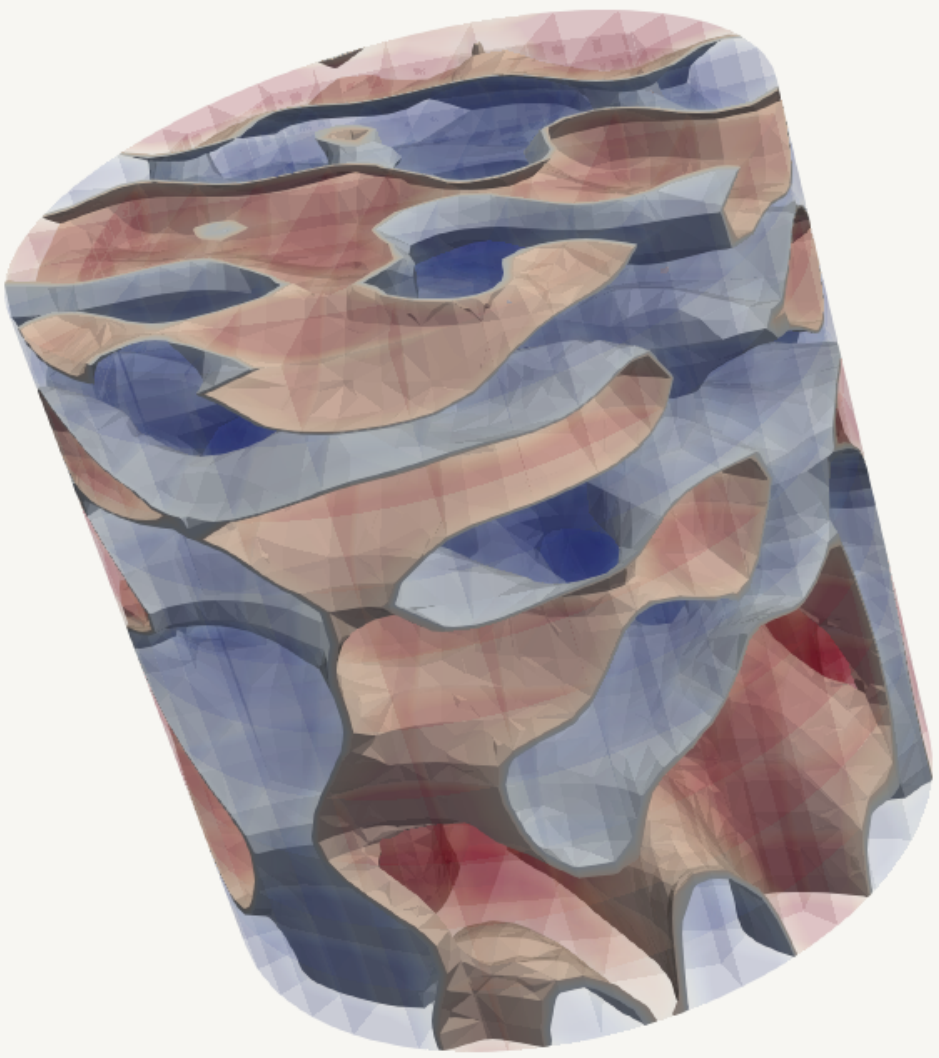
Refer to caption
(a) t=0t=0
Refer to caption
(b) t=10−4t=10^{-4}
Refer to caption
(c) t=10−3t=10^{-3}
Refer to caption
(d) t=10−2t=10^{-2}
Refer to caption
(e) t=0.1t=0.1
Refer to caption
(f) t=1.0t=1.0
Refer to caption
(g) t=10.0t=10.0
Figure 10: Evolution of the phases with time for the three dimensional spinoidal decomposition. Blue and red contours represent the equilibrium phases ϕ=−1\phi=-1 and ϕ=1\phi=1 respectively
Figure 11: Evolution of the free–energy ℱ\mathcal{F} with time for the three-dimensional spinodal decomposition simulation

6 Summary

We have developed a nodal Discontinuous Galerkin (DG) spectral element method (DGSEM) to solve the Cahn–Hilliard equation. We used the Gauss–Lobatto variant of the DG method to use the summation–by–parts simultaneous–approximation–term (SBP–SAT) property and showed that it is discretely stable. The spatial discretization uses the Bassi–Rebay 1 (BR1) method to couple inter–element fluxes, and the time discretization uses an efficient IMEX scheme. We first show the semi–discrete stability analysis (i.e. continuous in time), and later we show the fully–discrete one using the IMEX scheme. Both analyses show that the discrete free–energy is bounded in time by the initial value, which is in accordance with the continuous energy estimate. Lastly, we perform a convergence study of the scheme, we compare the scheme with previous results from the literature, and perform a simulation in three–dimensional curvilinear geometries, showing that the scheme is stable (i.e. its free–energy decreases) under all conditions tested herein as proved.

Acknowledgements.
The authors would like to thank Dr. Gustaaf Jacobs of the San Diego State University for his hospitality. This work was supported by a grant from the Simons Foundation (#426393, David Kopriva). This work has also been partially supported by Ministerio de Economía y Competitividad under the research grant TRA2015-67679-C2-2-R. The authors acknowledge the computer resources and technical assistance provided by the Centro de Supercomputación y Visualización de Madrid (CeSViMa).

Appendix A Stability analysis of the Crank–Nicolson scheme

It has been shown in (113) that the implicit Euler scheme used for Q→\vec{Q} in (89c) adds numerical dissipation that is proportional to the jumps in time Δ​Q→\Delta\vec{Q} squared,

−12​k​⟨𝒥​Δ​Q→,Δ​Q→⟩E,N⩽0.-\frac{1}{2}k\left\langle\mathcal{J}\Delta\vec{Q},\Delta\vec{Q}\right\rangle_{E,N}\leqslant 0. (131)

This dissipation can be effectively controlled using a linear combination of Q→n+1\vec{Q}^{n+1} and Q→n\vec{Q}^{n}. To show this, we define an intermediate state Q→θ\vec{Q}^{\theta},

Q→θ=K0​Q→n+1+(1−K0)​Q→n,\vec{Q}^{\theta}=K_{0}\vec{Q}^{n+1}+(1-K_{0})\vec{Q}^{n}, (132)

such that K0=1K_{0}=1 recovers backward Euler, K0=1/2K_{0}=1/2 is Crank–Nicolson, and K0=0K_{0}=0 is forward (explicit) Euler.

To study the stability, we consider (89c) and (91), where instead of Q→n+1\vec{Q}^{n+1} we use Q→θ\vec{Q}^{\theta} defined in (132),

⟨𝒥​Wθ,φW⟩E,N=\displaystyle\left\langle\mathcal{J}W^{\theta},\varphi_{W}\right\rangle_{E,N}= ⟨(⁡d​Ψ⁡d​Φ)n+S0​Φn+1−S0​Φn,𝒥​φW⟩E,N\displaystyle\left\langle\left(\frac{\mathop{}\!\mathrm{d}\Psi}{\mathop{}\!\mathrm{d}\Phi}\right)^{n}+S_{0}\Phi^{n+1}-S_{0}\Phi^{n},\mathcal{J}\varphi_{W}\right\rangle_{E,N}
−k∫∂E,NφW𝑸~⋆,θ⋅𝒏^dSξ+k⟨𝑸~θ,∇ξφW⟩E,N,\displaystyle-k\int_{\partial E,N}\varphi_{W}\tilde{\boldsymbol{Q}}^{\star,\theta}\cdot\hat{\boldsymbol{n}}\mathop{}\!\mathrm{d}S_{\xi}+k\left\langle\tilde{\boldsymbol{Q}}^{\theta},\nabla_{\xi}\varphi_{W}\right\rangle_{E,N}, (133a)
⟨𝒥​Δ​Q→Δ​t,φ→Q⟩E,N=\displaystyle\left\langle\mathcal{J}\frac{\Delta\vec{Q}}{\Delta t},\vec{\varphi}_{Q}\right\rangle_{E,N}= ∫∂E,N(Δ​Φ⋆Δ​t−Δ​ΦΔ​t)𝝋~Q⋅𝒏~dSξ+⟨∇ξ(Δ​Φ)Δ​t,𝝋~Q⟩E,N.\displaystyle\int_{\partial E,N}\left(\frac{\Delta\Phi^{\star}}{\Delta t}-\frac{\Delta\Phi}{\Delta t}\right)\tilde{\boldsymbol{\varphi}}_{Q}\cdot\tilde{\boldsymbol{n}}\mathop{}\!\mathrm{d}S_{\xi}+\left\langle\frac{\nabla_{\xi}\left(\Delta\Phi\right)}{\Delta t},\tilde{\boldsymbol{\varphi}}_{Q}\right\rangle_{E,N}. (133b)

We replace φ→Q→=Q→θ\vec{\varphi}_{\vec{Q}}=\vec{Q}^{\theta} in (133b), so that the left hand side is

⟨𝒥​Δ​Q→,Q→θ⟩E,N=⟨𝒥(Q→n+1−Q→n),K0Q→n+1+(1−K0)Q→n,⟩E,N=12​⟨𝒥​Q→n+1,Q→n+1⟩E,N−12​⟨𝒥​Q→n,Q→n⟩E,N+(K0−12)⟨𝒥ΔQ→,ΔQ→,⟩E,N.\begin{split}\left\langle\mathcal{J}\Delta\vec{Q},\vec{Q}^{\theta}\right\rangle_{E,N}=&\left\langle\mathcal{J}\left(\vec{Q}^{n+1}-\vec{Q}^{n}\right),K_{0}\vec{Q}^{n+1}+(1-K_{0})\vec{Q}^{n},\right\rangle_{E,N}\\ =&\frac{1}{2}\left\langle\mathcal{J}\vec{Q}^{n+1},\vec{Q}^{n+1}\right\rangle_{E,N}-\frac{1}{2}\left\langle\mathcal{J}\vec{Q}^{n},\vec{Q}^{n}\right\rangle_{E,N}\\ &+\left(K_{0}-\frac{1}{2}\right)\left\langle\mathcal{J}\Delta\vec{Q},\Delta\vec{Q},\right\rangle_{E,N}.\end{split} (134)

When we replace φW=Δ​ΦΔ​t\varphi_{W}=\frac{\Delta\Phi}{\Delta t}, we obtain the more general expression of (95),

⟨𝒥​Wθ,Δ​ΦΔ​t⟩E,N=⟨(⁡d​Ψ⁡d​Φ)n+S​Δ​Φ,𝒥​Δ​ΦΔ​t⟩E,N+k​⟨𝒥​Δ​Q→Δ​t,Q→θ⟩E,N−k​BTE,N​(Δ​ΦΔ​t,Q→θ).\begin{split}\left\langle\mathcal{J}W^{\theta},\frac{\Delta\Phi}{\Delta t}\right\rangle_{E,N}=&\left\langle\left(\frac{\mathop{}\!\mathrm{d}\Psi}{\mathop{}\!\mathrm{d}\Phi}\right)^{n}+S\Delta\Phi,\mathcal{J}\frac{\Delta\Phi}{\Delta t}\right\rangle_{E,N}+k\left\langle\mathcal{J}\frac{\Delta\vec{Q}}{\Delta t},\vec{Q}^{\theta}\right\rangle_{E,N}\\ &-k\text{BT}_{E,N}\left(\frac{\Delta\Phi}{\Delta t},\vec{Q}^{\theta}\right).\end{split} (135)

Following the rest of the steps in the fully–discrete analysis, which remain the same, we arrive to the same bound in (121), but with new IMEX dissipation, dissIMEXθ,E,N\text{diss}_{\text{IMEX}}^{\theta,E,N} in terms of K0K_{0}

dissIMEXθ,E,N=−⟨𝒥​Π,1⟩E,N−12​k​(K0−12)​⟨𝒥​Δ​Q→,Δ​Q→⟩E,N⩽0.\text{diss}^{\theta,E,N}_{\text{IMEX}}=-\left\langle\mathcal{J}\Pi,1\right\rangle_{E,N}-\frac{1}{2}k\left(K_{0}-\frac{1}{2}\right)\left\langle\mathcal{J}\Delta\vec{Q},\Delta\vec{Q}\right\rangle_{E,N}\leqslant 0. (136)

Thus, the amount of dissipation related to Q→\vec{Q} added by the implicit scheme varies linearly with K0K_{0}, and vanishes with K0=1/2K_{0}=1/2 (Crank–Nicolson scheme). Note that, with this approach, we cannot confirm that the explicit Euler is stable, which does not necessarily mean that it is unstable. The stability of the explicit Euler scheme is not analyzed in detail in this work as we consider it impractical due to the time step limitation imposed by the fourth order spatial derivate of the Cahn-Hilliard equation. In the numerical experiments, we set K0K_{0} to both 1 (implicit Euler) and 1/21/2 (Crank–Nicolson) to see whether it is enough with the dissipation provided by −⟨𝒥​Π,1⟩E,N-\left\langle\mathcal{J}\Pi,1\right\rangle_{E,N} and the physical dissipation for the approximation to be stable.

Appendix B Effect of interface stabilization in Q→⋆\vec{Q}^{\star}

We have only considered interface stabilization in the chemical potential gradient weak form, ℱ→⋆\vec{\mathcal{F}}^{\star}. We have not considered interface stabilization in the phase field gradient, Q→\vec{Q}, since we have found that it pollutes the free–energy ℱ\mathcal{F}. In this Appendix we show the effect of adding interface stabilization also to Q→⋆\vec{Q}^{\star},

Q→⋆={{Q}}−σq​⟦Φ⟧,\vec{Q}^{\star}=\left\{\!\!\left\{Q\right\}\!\!\right\}-\sigma_{q}\left\llbracket\Phi\right\rrbracket, (137)

where σq\sigma_{q} is a positive penalty parameter. When studying the boundary terms generated by (137),

BTE,N(Δ​ΦΔ​t,Q→n+1)=−σq∫∂e,N⟦Φn+1⟧⟦ΔΦ⟧dS,\text{BT}_{E,N}\left(\frac{\Delta\Phi}{\Delta t},\vec{Q}^{n+1}\right)=-\sigma_{q}\int_{\partial e,N}\left\llbracket\Phi^{n+1}\right\rrbracket\left\llbracket\Delta\Phi\right\rrbracket\mathop{}\!\mathrm{d}S, (138)

we find that (138) cannot be bounded. By rearranging,

−σ∫∂e,N⟦Φn+1⟧⟦ΔΦ⟧dS=−σq2∫∂e,N⟦Φn+1⟧2dS+σq2∫∂e,N⟦Φn⟧2dS−σq2∫∂e,N⟦Φn+1−Φn⟧2dS,\begin{split}-\sigma\int_{\partial e,N}\left\llbracket\Phi^{n+1}\right\rrbracket\left\llbracket\Delta\Phi\right\rrbracket\mathop{}\!\mathrm{d}S=&-\frac{\sigma_{q}}{2}\int_{\partial e,N}\left\llbracket\Phi^{n+1}\right\rrbracket^{2}\mathop{}\!\mathrm{d}S+\frac{\sigma_{q}}{2}\int_{\partial e,N}\left\llbracket\Phi^{n}\right\rrbracket^{2}\mathop{}\!\mathrm{d}S\\ &-\frac{\sigma_{q}}{2}\int_{\partial e,N}\left\llbracket\Phi^{n+1}-\Phi^{n}\right\rrbracket^{2}\mathop{}\!\mathrm{d}S,\end{split} (139)

we can see that by modifying the free–energy ℱ\mathcal{F} to

ℱσ=ℱ+σq2​∑interiorfaces∫f,N⟦Φn+1⟧2​⁡𝑑S,\mathcal{F}^{\sigma}=\mathcal{F}+\frac{\sigma_{q}}{2}\sum_{{\mathrm{interior}\atop\mathrm{faces}}}\int_{f,N}\left\llbracket\Phi^{n+1}\right\rrbracket^{2}\mathop{}\!\mathrm{d}S, (140)

then the dissipation is bounded and equal to

dissσ=−σq2∑interiorfaces∫f,N⟦Φn+1−Φn⟧2dS.\text{diss}_{\sigma}=-\frac{\sigma_{q}}{2}\sum_{{\mathrm{interior}\atop\mathrm{faces}}}\int_{f,N}\left\llbracket\Phi^{n+1}-\Phi^{n}\right\rrbracket^{2}\mathop{}\!\mathrm{d}S. (141)

Although the interface penalization contribution is always positive, and therefore the free–energy ℱ\mathcal{F} is bounded in time, we cannot confirm that the free–energy is strictly monotonic in time. In most practical cases it is, and other methods that rely on this stabilization (e.g. the interior penalty method 1978:Wheeler) have been found by us to work well in practice with the Cahn–Hilliard equation.

References

  • (1) D. Lee, J. Kim, Comparison study of the conservative Allen–Cahn and the Cahn–Hilliard equations, Mathematics and Computers in Simulation 119 (2016) 35 – 56.
  • (2) J. W. Cahn, J. E. Hilliard, Free energy of a nonuniform system. I. Interfacial free energy, The Journal of Chemical Physics 28 (2) (1958) 258–267.
  • (3) Y. Xia, Y. Xu, C.-W. Shu, Local discontinuous Galerkin methods for the Cahn–Hilliard type equations, Journal of Computational Physics 227 (1) (2007) 472 – 491.
  • (4) D. A. Kopriva, A polynomial spectral calculus for analysis of DG spectral element methods, Springer International Publishing, Cham, 2017, pp. 21–40.
  • (5) D.A. Kopriva and G.J. Gassner, An energy stable discontinuous Galerkin spectral element discretization for variable coefficient advection problems, SIAM Journal on Scientific Computing 36 (4) (2014) A2076–A2099.
  • (6) J. Manzanero, G. Rubio, E. Ferrer, E. Valero and D.A. Kopriva, Insights on aliasing driven instabilities for advection equations with application to Gauss-Lobatto discontinuous Galerkin methods, Journal of Scientific Computing 75 (3) (2018) 1262–1281.
  • (7) G.J. Gassner, A skew-symmetric discontinuous Galerkin spectral element discretization and its relation to SBP-SAT finite difference methods, SIAM Journal on Scientific Computing 35 (3) (2013) 1233–1256.
  • (8) G.J. Gassner, A.R. Winters, F.J. Hinderlang, D.A. Kopriva, The BR1 scheme is stable for the compressible Navier–Stokes equations, Journal of Scientific Computing 77 (1) (2018) 154–200.
  • (9) G. J. Gassner, A. R. Winters, D. A. Kopriva, A well balanced and entropy conservative discontinuous Galerkin spectral element method for the shallow water equations, Applied Mathematics and Computation 272 (2016) 291 – 308, recent Advances in Numerical Methods for Hyperbolic Partial Differential Equations.
  • (10) G. J. Gassner, A. R. Winters, D. A. Kopriva, Split form nodal discontinuous Galerkin schemes with summation-by-parts property for the compressible Euler equations, Journal of Computational Physics 327 (Supplement C) (2016) 39 – 66.
  • (11) A.R. Winters and G.J. Gassner, Affordable, entropy conserving and entropy stable flux functions for the ideal MHD equations, Journal of Computational Physics 304 (2016) 72 – 108.
  • (12) S. Dong, Multiphase flows of N immiscible incompressible fluids: A reduction-consistent and thermodynamically-consistent formulation and associated algorithm, Journal of Computational Physics 361 (2018) 1 – 49.
  • (13) A. Debussche, L. Dettori, On the Cahn-Hilliard equation with a logarithmic free energy, Nonlinear Analysis: Theory, Methods & Applications 24 (10) (1995) 1491 – 1514.
  • (14) D.A. Kopriva, Implementing spectral methods for partial differential equations, Springer Netherlands, 2009.
  • (15) D. A. Kopriva, Metric identities and the discontinuous spectral element method on curvilinear meshes, Journal of Scientific Computing 26 (3) (2006) 301.
  • (16) J. Manzanero, A.M. Rueda–Ramírez, G. Rubio and E. Ferrer, The Bassi Rebay 1 scheme is a special case of the Symmetric Interior Penalty formulation for discontinuous Galerkin discretisations with Gauss–Lobatto points, Journal of Computational Physics 363 (2018) 1 – 10.
  • (17) M. Kästner, P. Metsch, and R. de Borst, Isogeometric analysis of the Cahn–Hilliard equation– a convergence study, Journal of Computational Physics 305 (2016) 360 – 371.
  • (18) M. Ainsworth, Dispersive and dissipative behaviour of high order discontinuous Galerkin finite element methods, J. Comput. Phys. 198 (1) (2004) 106–130.
  • (19) A. Jokisaari, P. Voorhees, J. Guyer, J. Warren, O. Heinonen, Benchmark problems for numerical implementations of phase field models, Computational Materials Science 126.
  • (20) M.F. Wheeler, An Elliptic Collocation-Finite Element Method with Interior Penalties, SIAM Journal on Numerical Analysis 15 (1) (1978) 152–161.