跳到论文正文
W Papers独立论文阅读器 arXiv:1902.08055 论文正文 计算阅读时间 · 0%
引用这篇论文根据当前论文元数据生成,正式投稿前建议核对。


License: arXiv.org perpetual non-exclusive license
arXiv:1902.08055v3 [cs.LO] 11 Feb 2020

Schematic Refutations of Formula Schemata

David Cerna Affiliation: Institute for Formal Methods and Verification, JKU, Linz, Austria
Research Institute for Symbolic Computation, JKU, Hagenberg, Austria
E-mail david.cerna@jku.at,david.cerna@risc.jku.at
   Alexander Leitsch Affiliation: Institute of Logic and Computation, TU Wien, Vienna, Austria E-mail leitsch@logic.at    Anela Lolic Affiliation: Institute of Logic and Computation, TU Wien, Vienna, Austria E-mail anela@logic.at
Abstract

Proof schemata are infinite sequences of proofs which are defined inductively. In this paper we present a general framework for schemata of terms, formulas and unifiers and define a resolution calculus for schemata of quantifier-free formulas. The new calculus generalizes and improves former approaches to schematic deduction. As an application of the method we present a schematic refutation formalizing a proof of a weak form of the pigeon hole principle.

Keywords: 
schema resolution induction.

1 Introduction

Recursive definitions of functions play a central role in computer science, particularly in functional programming. While recursive definitions of proofs are less common they are of increasing importance in automated proof analysis. Proof schemata, i.e. recursively defined infinite sequences of proofs, serve as an alternative formulation of induction. Prior to the formalization of the concept, an analysis of Fürstenberg’s proof of the infinitude of primes [3] suggested the need for a formalism quite close to the type of proof schemata we will discuss in this paper. The underlying method for this analysis was CERES [5] (cut-elimination by resolution) which, unlike reductive cut-elimination, can be applied to recursively defined proofs by extracting a schematic unsatisfiable formula and constructing a recursively defined refutation. Moreover, Herbrand’s theorem can be extended to an expressive fragment of proof schemata, that is those formalizing kk-induction [10, 14]. Unfortunately, the construction of recursively defined refutations is a highly complex task. In previous work [14] a superposition calculus for certain types of formulas was used for the construction of refutation schemata, but only works for a weak fragment of arithmetic and is hard to use interactively.

The key to proof analysis using CERES in a first-order setting is not the particularities of the method itself, but the fact that it provides a bridge between automated deduction and proof theory. In the schematic setting, where the proofs are recursively defined, a bridge over the chasm has been provided  [10, 14], but there has not been much development on the other side to reap the benefits of. The few existing results about automated deduction for recursively defined formulas barely provide the necessary expressive power to analyse significant mathematical argumentation. Applying the earlier constructions to a weak mathematical statement such as the eventually constant schema required much more work than the value of the provided insights [8]. The resolution calculus we introduce in this work generalizes resolution and the first-order language in such a way that it provides an excellent environment for carrying out investigations into decidable fragments of schematic propositional formulas beyond those that are known. Furthermore, concerning the general unsatisfiability problem for schematic formulas, our formalism provides a perfect setting for interactive proof construction.

Proof schema is not the first alternative formalization of induction with respect to Peano arithmetic [17]. However, all other existing examples [6, 7, 15] that provide calculi for induction together with a cut-elimination procedure do not allow the extraction of Herbrand sequents11 1 Herbrand sequents allow the representation of the propositional content of first-order proofs. [12, 17] and thus Herbrand’s theorem cannot be realized. In contrast, in [14] finite representations of infinite sequences of Herbrand sequents are constructed, so-called Herbrand systems. Of course, such objects do not describe finite sets of ground instances, though instantiating the free parameters of Herbrand systems does result in sequents derivable from a finite set of ground instances.

The formalism developed in this paper extends and improves the formal framework for refuting formula schemata in [10, 14] in several ways: 1. The new calculus can deal with arbitrary quantifier-free formula schemata (not only with clause schemata), 2. we extend the schematic formalism to multiple parameters (in [10] and in [14] only schemata defined via one parameter were admitted); 3. we strongly extend the recursive proof specifications by allowing mutual recursion (formalizable by so-called call graphs). Note that in [10] a complicated schematic clause definition was used, while the schematic refutations in [14] were based on negation normal forms and on a complicated translation to the nn-clause calculus. Moreover, the new method presented in this paper provides a simple, powerful and elegant formalism for interactive use. The expressivity of the method is illustrated by an application to a (weak) version of the pigeon hole principle.

2 A Motivational Example

In [8], proof analysis of a mathematically simple statement, the Eventually Constant Schema, was performed using an early formalism developed for schematic proof analysis [10]. The Eventually Constant Schema states that any monotonically decreasing function with a finite range is eventually constant. The property of being eventually constant may be formally written as follows:

∃x​∀y⁡(x≤y→f⁡(x)=f⁡(y)),\exists x\forall y(x\leq y\rightarrow f(x)=f(y)), (1)

where ff is an uninterpreted function symbol with the following property

∀x⁡(⋁i=0nf⁡(x)=i)\forall x\left(\bigvee_{i=0}^{n}f(x)=i\right)

for some n∈ℕn\in\mathbb{N}. The method defined in [10] requires a strong quantifier-free end sequent, thus implying the proof must be skolemized. The skolemized formulation of the eventually constant property is ∃x⁡(x≤g⁡(x)→f⁡(x)=f⁡(g⁡(x)))\exists x(x\leq g(x)\rightarrow f(x)=f(g(x))) where gg is the introduced Skolem function. The proof presented in [8] used a sequence of Σ2\Sigma_{2}-cuts

∃x​∀y⁡(((x≤y)⇒n+1=f⁡(y))∨f⁡(y)<n+1).\exists x\forall y(((x\leq y)\Rightarrow n+1=f(y))\vee f(y)<n+1).

Also, the Skolem function was left uninterpreted for the proof analysis. The resulting cut-structure, when extracted as an unsatisfiable clause set, has a fairly simple refutation. Thus, with the aid of automated theorem provers, a schema of refutations was constructed.

The use of an uninterpreted Skolem function greatly simplified the construction presented in [8]. In this paper we will interpret the function gg as the successor function. Note that using the axioms presented in [8] the following statement

∀x⁡(⋁i=0nf⁡(x)=i)⊢∃x⁡(f⁡(x)=f⁡(𝑠𝑢𝑐⁡(x)))\forall x\left(\bigvee_{i=0}^{n}f(x)=i\right)\vdash\exists x(f(x)=f(\mathit{suc}(x)))

is not provable. Note that we drop the implication of Equation 1 and the antecedent of the implication given that x≤𝑠𝑢𝑐⁡(x)x\leq\mathit{suc}(x) is a trivial property of the successor function. However, using an alternative set of axioms and a weaker cut we can prove this statement. The additional axioms are as follows:

f⁡(x)=i⊢f⁡(x)<s⁡(k),for 0≤i≤k<n f(x)=i\vdash f(x)<s(k)\ ,\ \mbox{for $0\leq i\leq k<n$ }
f⁡(𝑠𝑢𝑐⁡(x))=i⊢f⁡(x)<s⁡(k),for 0≤i≤k<n f(\mathit{suc}(x))=i\vdash f(x)<s(k)\ ,\ \mbox{for $0\leq i\leq k<n$ }
f(x)=k,f(𝑠𝑢𝑐(x))=k⊢f(x)=f(𝑠𝑢𝑐(x)),for 0≤k≤n f(x)=k,f(\mathit{suc}(x))=k\vdash f(x)=f(\mathit{suc}(x))\ ,\ \mbox{for $0\leq k\leq n$ }
f⁡(0)<0⊢f(0)<0\vdash
f(𝑠𝑢𝑐(x))<s(k)⊢f(𝑠𝑢𝑐(x))=k,f(x)<k,for 0≤k≤n f(\mathit{suc}(x))<s(k)\vdash f(\mathit{suc}(x))=k,f(x)<k\ ,\ \mbox{for $0\leq k\leq n$ }
f(x)<s(k)⊢f(x)=k,f(x)<k,for 0≤k<n f(x)<s(k)\vdash f(x)=k,f(x)<k\ ,\ \mbox{for $0\leq k<n$ }

For the most part these axioms are harmless, however f⁡(𝑠𝑢𝑐⁡(x))<s⁡(k)⊢f⁡(𝑠𝑢𝑐⁡(x))=k,f⁡(x)<kf(\mathit{suc}(x))<s(k)\vdash f(\mathit{suc}(x))=k,f(x)<k implies that ff has some monotonicity properties similar to the eventually constant schema. For all values yy in the range larger than xx, either f⁡(y)=nf(y)=n or f⁡(y)<nf(y)<n. Our axioms imply that once f⁡(y)<nf(y)<n all values z>yz>y are mapped to values of the range less than nn. Being that our proof enforces this property using the following Δ2\Delta_{2}-cut formula we are guaranteed to reach a value in the domain above which ff is constant. The cut formula is as follows:

∃x⁡(f⁡(x)=k∧k=f⁡(𝑠𝑢𝑐⁡(x)))∨∀x⁡(f⁡(x)<k),for ​0≤k≤n.\exists x(f(x)=k\wedge k=f(\mathit{suc}(x)))\vee\forall x(f(x)<k)\ ,\ \mbox{for }0\leq k\leq n.

One additional point which the reader might notice is that we use what seems to be the less than relation and equality relation of the natural numbers, but do not concern ourselves with substitutivity of equality nor transitivity of <<. While including these properties will change the formal proof we present below, the argument will still require a free numeric parameter denoting the size of the range of ff and the number of positions we require to map to the same value.

We will refer to this version of the eventually constant schema as the successor eventually constant schema. While this results in a new formulation of the eventually constant schema under an interpretation of the Skolem function as the successor function, we have not taken complete advantage of this new interpretation yet in that this re-formulation is actually of lower complexity than the eventually constant schema. For example in Figure 1 we provide the output of Peltier’s superposition induction prover[2] when ran on the clausified form of thee cut structure of the successor eventually constant schema. The existence of this derivation implies that the proof analysis method of [14] may be applied to the successor eventually constant schema. Unfortunately, the prover does not find the invariant discovered in [8], but this may have more to do with the choice of axioms rather than the statement being beyond the capabilities of the prover.

============================== PROOF =================================

% Proof 1 at 0.017 (+ 0.000) seconds.
% Given clauses 73.

% number of calls to fixpoint : 3
 S_init  :
 (51:  [ EQ(v0,f(h(v1))) | LE(f(v1),v0) if  n = s(v0) ].
50:  [ EQ(v0,f(v1)) | LE(f(v1),v0) if  n = s(v0) ].
33:  [ PHI(v0,v1) if  n = s(v0) ].
)
 S_loop  :
 (82:  [ EQ(v0,f(h(v1))) | LE(f(v1),v0) if  n = s(s(v0)) ].
80:  [ EQ(v0,f(v1)) | LE(f(v1),v0) if  n = s(s(v0)) ].
53:  [ PHI(v0,v1) if  n = s(s(v0)) ].
)
 The empty clauses  :
 (45:  [  n = 0 ].
81:  [  n = s(0) ].
112:  [  n = s(s(0)) ].
) max_rank 2

============================== end of proof ==========================
Figure 1: output of Peltier et al.’s Prover9 extension [13].

We can strengthen the successor eventually constant schema beyond the capabilities of [13] easily by adding a second parameter as follows:

∀x⁡(⋁i=0nf⁡(x)=i)⊢∃x⁡(⋀i=0mf⁡(x)=f⁡(𝑠𝑢𝑐i​(x))).\forall x\left(\bigvee_{i=0}^{n}f(x)=i\right)\vdash\exists x(\bigwedge_{i=0}^{m}f(x)=f(\mathit{suc}^{i}(x))).

We refer to this problem as the mm-successor eventually constant schema. Applying this transformation to the the eventually constant schema of [8] is not so trivial being that the axioms used to construct the proof do not easy generalize. However, for the successor eventually constant schema the generalization is trivial and is provided below:

f⁡(𝑠𝑢𝑐r​(x))=i⊢f⁡(x)<s⁡(k),for 0≤i≤k≤n and 0≤r≤mf(\mathit{suc}^{r}(x))=i\vdash f(x)<s(k)\ ,\ \mbox{for $0\leq i\leq k\leq n$ and $0\leq r\leq m$}
f(x)=k,f(𝑠𝑢𝑐r(x))=k⊢f(x)=f(𝑠𝑢𝑐r(x)),for 0≤k≤n and 0<r≤mf(x)=k,f(\mathit{suc}^{r}(x))=k\vdash f(x)=f(\mathit{suc}^{r}(x))\ ,\ \mbox{for $0\leq k\leq n$ and $0<r\leq m$}
f⁡(0)<0⊢f(0)<0\vdash
f(𝑠𝑢𝑐r(x))<s(k)⊢f(𝑠𝑢𝑐r(x))=k,f(x)<k,for 0≤k≤n and 0≤r≤m,f(\mathit{suc}^{r}(x))<s(k)\vdash f(\mathit{suc}^{r}(x))=k,f(x)<k\ ,\ \mbox{for $0\leq k\leq n$ and $0\leq r\leq m$},

where 𝑠𝑢𝑐0​(x)=x\mathit{suc}^{0}(x)=x. Furthermore, the cut formula can be trivial extended as follows:

∃x⁡(⋀i=0mf⁡(𝑠𝑢𝑐i​(x))=k)∨∀x⁡(f⁡(x)<k),for ​0≤k≤n.\exists x(\bigwedge_{i=0}^{m}f(\mathit{suc}^{i}(x))=k)\vee\forall x(f(x)<k)\ ,\ \mbox{for }0\leq k\leq n.

Given that the mm-successor eventually constant schema contains two parameters it is beyond the capabilities of [13]. Interesting enough, the prover can find invariants for each value of mm in terms of nn, though, these invariant get impressively large quite quickly. The cut structure of the mm-successor eventually constant schema by be extracted as an inductive definition of an unsatisfiable negation normal form formula. We provide this definition by rewrite rules below:

O⁡(n,m)≡\displaystyle O(n,m)\equiv D⁡(n,m)∧P⁡(n,m)\displaystyle D(n,m)\wedge\ P(n,m)
C⁡(y,n,0)≡\displaystyle C(y,n,0)\equiv f⁡(S⁡(0,y))≠n\displaystyle f(S(0,y))\not=n
C⁡(y,n,s⁡(m))≡\displaystyle C(y,n,s(m))\equiv f⁡(S⁡(s⁡(m),y))≠n∨C⁡(y,n,m)\displaystyle f(S(s(m),y))\not=n\ \vee\ C(y,n,m)
T⁡(n,0)≡\displaystyle T(n,0)\equiv ∀x⁡(f⁡(S⁡(0,x))≮s⁡(n)∨f⁡(S⁡(0,x))=n∨f⁡(x)<n)\displaystyle\forall x(f(S(0,x))\not<s(n)\ \vee\ f(S(0,x))=n\ \vee\ f(x)<n)
T⁡(n,s⁡(m))≡\displaystyle T(n,s(m))\equiv ∀x⁡(f⁡(S⁡(s⁡(m),x))≮s⁡(n)∨f⁡(S⁡(s⁡(m),x))=n∨f⁡(x)<n)\displaystyle\forall x(f(S(s(m),x))\not<s(n)\ \vee\ f(S(s(m),x))=n\vee f(x)<n)
∧T⁡(n,m)\displaystyle\wedge\ T(n,m)
P⁡(0,m)≡\displaystyle P(0,m)\equiv ∀x⁡(C⁡(x,0,m))∧f⁡(a)≮0\displaystyle\forall x(C(x,0,m))\ \wedge\ f(a)\not<0
P⁡(s⁡(n),m)≡\displaystyle P(s(n),m)\equiv (∀x⁡(C⁡(x,s⁡(n),m))∧(T⁡(n,m))∧P⁡(n,m)CLOSE\displaystyle(\forall x(C(x,s(n),m))\ \wedge(T(n,m))\ \wedge\ P(n,m)
D⁡(n,0)≡\displaystyle D(n,0)\equiv ∀x⁡(f⁡(S⁡(0,x))=n∨f⁡(x)<n)\displaystyle\forall x(f(S(0,x))=n\ \vee\ f(x)<n)
D⁡(n,s⁡(m))≡\displaystyle D(n,s(m))\equiv ∀x⁡(f⁡(S⁡(s⁡(m),x))=n∨f⁡(x)<n)∧D⁡(n,m)\displaystyle\forall x(f(S(s(m),x))=n\ \vee\ f(x)<n)\wedge\ D(n,m)
S⁡(0,y)≡\displaystyle S(0,y)\equiv y\displaystyle y
S⁡(s⁡(n),y)≡\displaystyle S(s(n),y)\equiv 𝑠𝑢𝑐⁡(S⁡(s⁡(n),y))\displaystyle\mathit{suc}(S(s(n),y))

where aa is some arbitrary constant. We will show how our new formalism can provide a finite representation of the refutations of inductive definition even though the refutation requires mutual recursion as well as multiple parameters (six in total) to state finitely.

3 Schematic Language

We work in a two-sorted version of classical first-order logic. The first sort we consider is ω\omega, in which every ground term normalizes to a numeral, i.e. a term inductively constructable by N⇒s⁡(N)| 0N\Rightarrow s(N)\ |\ 0, such that s⁡(N)≠0s(N)\not=0 and s⁡(N)=s⁡(N′)→N=N′s(N)=s(N^{\prime})\to N=N^{\prime}. Natural numbers (ℕ\mathbb{N}) will be denoted by lower-case Greek letters (α\alpha, β\beta, γ\gamma, etc); The numeral sα​0s^{\alpha}0, α∈ℕ\alpha\in\mathbb{N}, will be written as α¯\bar{\alpha}. The set of numerals is denoted by 𝑁𝑢𝑚{\it Num}. Furthermore, the ω\omega sort includes a countable set of variables 𝒩\mathcal{N} called parameters. We denote parameters by n,m,n1,n2,…,m1,m2,…n,m,n_{1},n_{2},\ldots,m_{1},m_{2},\ldots. The set of parameters occurring in an expression EE is denoted by 𝒩⁡(E)\mathcal{N}(E).

The second sort, the ι\iota-sort (individuals), is a standard first-order term language extended by defined function symbols. Defined function symbols, i.e. primitive recursively defined functions, are differentiated from standard function symbols by adding a ⋅^\hat{\cdot}.

Variables of the ι\iota-sort are what we refer to as global variables. Global variables are indexed by terms of the ω\omega-sort and are of type ωα→ι\omega^{\alpha}\to\iota for α≥0\alpha\geq 0. The set of global variables will be denoted by VGV^{G}. Given a sequence of ω\omega terms t→\overrightarrow{t} of length α\alpha and a global variable X of type ωα→ι\omega^{\alpha}\to\iota, we will refer to the ι\iota terms X⁡(t→)X(\overrightarrow{t}) as V-terms over XX. The set of individual variables VιV^{\iota} consists of objects of the form X⁡(t→)X(\overrightarrow{t}) where t→\overrightarrow{t} is a tuple of numerals. Additionally we introduce VFV^{F}, the set of formula variables of type oo which aid the construction defined predicate symbols.

For terms we consider the set of function symbols of type τ\tau, ℱτ{\cal F}^{\tau}. The set of defined function symbols of type τ\tau is denoted by ℱ^τ\hat{{\cal F}}^{\tau}. The types τ\tau are either of the form ωα→ω\omega^{\alpha}\to\omega (for α∈ω\alpha\in\omega) which we call numeric types or of type ια→ι\iota^{\alpha}\to\iota for α≥0\alpha\geq 0 which we call individual types. We distinguish ℱ^ω\hat{{\cal F}}_{\omega} - the set of all defined function symbols of numeric type and ℱ^ι\hat{{\cal F}}_{\iota} - the set of all defined function symbols of individual type. We define ℱω={0¯}{\cal F}^{\omega}=\{\bar{0}\}, ℱω→ω={s}{\cal F}^{\omega\to\omega}=\{s\}, and ℱτ=∅{\cal F}^{\tau}=\emptyset for α>1\alpha>1. We leave the symbol sets of complex ω\omega types empty so that normalization of a ground term always results in a numeral. For the same reason the only constants of type ω\omega are 00 and ss. Basic functions such as projections will be introduced as defined function symbols. For all other types τ\tau the set ℱτ{\cal F}^{\tau} is infinite. This extends to the defined symbols of any type, i.e. ℱ^τ\hat{{\cal F}}^{\tau} is infinite. For defined function symbols we make use of global variables: the types τ\tau are (ωγ1→ι)×…×(ωγα→ι)×ωβ→ι(\omega^{\gamma_{1}}\to\iota)\times\ldots\times(\omega^{\gamma_{\alpha}}\to\iota)\times\omega^{\beta}\to\iota for α≥0\alpha\geq 0 and γi>0\gamma_{i}>0 for i∈{1,…,α}i\in\{1,\ldots,\alpha\}. The symbols in ℱ^ω\hat{{\cal F}}_{\omega} and ℱ^ι\hat{{\cal F}}_{\iota} are partially ordered by <ℱ^<_{\hat{{\cal F}}} where <ℱ^<_{\hat{{\cal F}}} is irreflexive, transitive and Noetherian.

We define a similar signature for predicate symbols of type τ\tau, where 𝒫iτ{\cal P}^{\tau}_{i} is the (infinite) set of predicate symbols of type τ\tau; the set of defined predicate symbols of type τ\tau is denoted by 𝒫^τ\hat{{\cal P}}^{\tau}. For ordinary (α\alpha-ary) predicate symbols the types are ια→o\iota^{\alpha}\to o, for α≥0\alpha\geq 0 as usual. Like for defined function symbols we make use of global and context variables for defined predicate symbols: the types τ\tau are (ωγ1→ι)×…×(ωγα→ι)×ωβ→o(\omega^{\gamma_{1}}\to\iota)\times\ldots\times(\omega^{\gamma_{\alpha}}\to\iota)\times\omega^{\beta}\to o for α≥0\alpha\geq 0 and γi>0\gamma_{i}>0 for i∈{1,…,α}i\in\{1,\ldots,\alpha\}. The symbols in 𝒫^\hat{{\cal P}} are partially ordered by <𝒫^<_{\hat{{\cal P}}} where <𝒫^<_{\hat{{\cal P}}} is irreflexive, transitive and Noetherian.

For the term language we consider ω\omega-terms of type ω\omega and ι\iota-terms of type ι\iota. Both term sets are defined via function symbols and defined function symbols.

Definition 1 (ω\omega-terms TωT^{\omega} )

  • (1)

    0¯∈Tω,𝒩⊆Tω\bar{0}\in T^{\omega},\ \mathcal{N}\subseteq T^{\omega}, and if t∈Tωt\in T^{\omega} then s⁡(t)∈Tωs(t)\in T^{\omega},

  • (2)

    if f^∈ℱ^ωτ\hat{f}\in\hat{{\cal F}}_{\omega}^{\tau} for τ=ωα→ω\tau=\omega^{\alpha}\to\omega and t1,…,tα∈Tωt_{1},\ldots,t_{\alpha}\in T^{\omega} then f^​(t1,…,tα)∈Tω\hat{f}(t_{1},\ldots,t_{\alpha})\in T^{\omega}.

The set T0ωT^{\omega}_{0} denotes terms constructed using (1). Note that the set of parameter-free terms in T0ωT^{\omega}_{0} is 𝑁𝑢𝑚{\it Num}, the set of numerals.

For every defined function symbol f^∈ℱ^ω\hat{f}\in\hat{{\cal F}}_{\omega} there exists a set of defining equations D⁡(f^)D(\hat{f}) which expresses a primitive recursive definition of f^\hat{f}.

Definition 2 (defining equations for numeric function symbols)

For every f^∈ℱ^ω\hat{f}\in\hat{{\cal F}}_{\omega}, f^:ωα+1→ω\hat{f}\colon\omega^{\alpha+1}\to\omega we define a set D⁡(f^)D(\hat{f}) consisting of two equations:

f^(n1,…,nα,0¯)=tB,f^(n1,…,nα,s(m))=tS{k←f^(n1,…,nα,m)},\hat{f}(n_{1},\ldots,n_{\alpha},\overline{0})=t_{B},\quad\hat{f}(n_{1},\ldots,n_{\alpha},s(m))=t_{S}\{k\leftarrow\hat{f}(n_{1},\ldots,n_{\alpha},m)\},

where for minimal f^\hat{f} tB,tS∈T0ωt_{B},t_{S}\in T^{\omega}_{0}; for nonminimal f^\hat{f} tB,tS∈Tωt_{B},t_{S}\in T^{\omega} where tB,tSt_{B},t_{S} may contain only defined function symbols smaller than f^\hat{f} in <ℱ^<_{\hat{{\cal F}}}. Furthermore 𝒩⁡(tB)⊆{n1,…,nα}\mathcal{N}(t_{B})\subseteq\{n_{1},\ldots,n_{\alpha}\}, and 𝒩⁡(tS)⊆{n1,…,nα}∪{m,k}\mathcal{N}(t_{S})\subseteq\{n_{1},\ldots,n_{\alpha}\}\cup\{m,k\}.

We define D⁡(ℱ^ω)=⋃{D⁡(f^)∣f^∈ℱ^ω}D(\hat{{\cal F}}_{\omega})=\bigcup\{D(\hat{f})\mid\hat{f}\in\hat{{\cal F}}_{\omega}\}, which is the set of all defining equations in the numeric types.

Example 1

For p^∈ℱ^ω→ω\widehat{p}\in\hat{{\cal F}}^{\omega\to\omega}, D⁡(p^)={p^​(0¯)=0¯,p^​(s⁡(m))=m}D(\widehat{p})=\left\{\widehat{p}(\bar{0})=\bar{0},\ \widehat{p}(s(m))=m\right\}, tB=0¯t_{B}=\bar{0}, ts=mt_{s}=m.
Let f^,g^∈ℱ^τ\hat{f},\hat{g}\in\hat{{\cal F}}^{\tau} for τ=ω×ω→ω\tau=\omega\times\omega\to\omega, f^\hat{f} be minimal and f^<ℱ^g^\hat{f}<_{\hat{{\cal F}}}\hat{g}. We define D⁡(f^)D(\hat{f}) as

f^(n,0¯)=tB,f^(n,s(m))=tS{k←f^(n,m)}\hat{f}(n,\bar{0})=t_{B},\quad\hat{f}(n,s(m))=t_{S}\{k\leftarrow\hat{f}(n,m)\}

for tB=nt_{B}=n and tS=s⁡(k)t_{S}=s(k). Then, obviously, f^\hat{f} defines ++.
Now we define D⁡(g^)D(\hat{g}) as

g^(n,0¯)=tB′,g^(n,s(m))=tS′{k←g^(n,m)}\hat{g}(n,\bar{0})=t^{\prime}_{B},\quad\hat{g}(n,s(m))=t^{\prime}_{S}\{k\leftarrow\hat{g}(n,m)\}

where tB′=0¯t^{\prime}_{B}=\bar{0} and tS′=f^​(n,k)t^{\prime}_{S}=\hat{f}(n,k). Then g^\hat{g} defines ∗*.

It is easy to see that, given any parameter assignment, all terms in TωT^{\omega} evaluate to numerals.

Definition 3 (parameter assignment)

A function σ:𝒩→𝑁𝑢𝑚\sigma\colon\mathcal{N}\to{\it Num} is called a parameter assigment. σ\sigma is extended to terms homomorphically:

  • •

    σ⁡(β¯)=β¯\sigma(\bar{\beta})=\bar{\beta} for numerals β¯\bar{\beta}.

  • •

    σ⁡(f^​(t1,…,tα))=f^​(σ⁡(t1),…,σ⁡(tα))\sigma(\hat{f}(t_{1},\ldots,t_{\alpha}))=\hat{f}(\sigma(t_{1}),\ldots,\sigma(t_{\alpha})) for f^:ωα→ω\hat{f}\colon\omega^{\alpha}\to\omega and t1,…,tα∈Tωt_{1},\ldots,t_{\alpha}\in T^{\omega}.

The set of all parameter assigments is denoted by 𝒮{\cal S}.

To simplify notation we use the following convention: if σ∈𝒮\sigma\in{\cal S} and n→=(n1,…CLOSE,\vec{n}=(n_{1},\ldots, OPENnα)n_{\alpha}) we write σ⁡(n→)\sigma(\vec{n}) for (σ⁡(n1),…CLOSE,(\sigma(n_{1}),\ldots, OPENσ⁡(nα))\sigma(n_{\alpha})).

Definition 4 (rewrite system R⁡(ℱ^ω)R(\hat{{\cal F}}_{\omega}))

Let f^∈ℱ^ω\hat{f}\in\hat{{\cal F}}_{\omega}. Then R⁡(f^)R(\hat{f}) is the set of the following rewrite rules obtained from D⁡(f^)D(\hat{f}):

f^(n1,…,nα,0^)→tB,f^(n1,…,nα,s(m))→tS{k←f^(n1,…,nα,m)}\hat{f}(n_{1},\ldots,n_{\alpha},\hat{0})\to t_{B},\quad\hat{f}(n_{1},\ldots,n_{\alpha},s(m))\to t_{S}\{k\leftarrow\hat{f}(n_{1},\ldots,n_{\alpha},m)\}

R⁡(ℱ^ω)=⋃{R⁡(f^)∣f^∈ℱ^ω}R(\hat{{\cal F}}_{\omega})=\bigcup\{R(\hat{f})\mid\hat{f}\in\hat{{\cal F}}_{\omega}\}. When a numeric term s∈Tωs\in T^{\omega} rewrites to tt under R⁡(ℱ^ω)R(\hat{{\cal F}}_{\omega}) we write s→ωts\to_{\omega}t.

Proposition 1

.

  • •

    R⁡(ℱ^ω)R(\hat{{\cal F}}_{\omega}) is a canonical rewrite system.

  • •

    Let t∈Tωt\in T^{\omega} and σ∈𝒮\sigma\in{\cal S}. Then the (unique) normal form of σ⁡(t)\sigma(t) under R⁡(ℱ^ω)R(\hat{{\cal F}}_{\omega}) (denoted by σ(t)↓ω\sigma(t)\hskip-2.84544pt\downarrow_{\omega}) is a numeral .

Proof

Straightforward: termination and confluence of R⁡(ℱ^ωCLOSER(\hat{{\cal F}}_{\omega}) are well known. In particular 0¯,s\bar{0},s and R⁡(ℱ^)R(\hat{{\cal F}}) define a language for computing the set of primitive recursive functions; in particular the recursions are well founded. A formal proof of termination requires double induction on <ℱ^<_{\hat{{\cal F}}} and the value of the recursion parameter.

An important remark concerning global variables and normalization is as follows: Let t1,⋯tα,s1,⋯sα∈ωt_{1},\cdots t_{\alpha},s_{1},\cdots s_{\alpha}\in\omega, X,Y∈VGX,Y\in V^{G} of type ωα→ι\omega^{\alpha}\to\iota, then we say X(t1,⋯tα)=Y(s1,⋯sα)X(t_{1},\cdots t_{\alpha})=Y(s_{1},\cdots s_{\alpha}) iff X=YX=Y and for any parameter assignment σ\sigma we have σ(ti)↓ω=σ(si)↓ω\sigma(t_{i})\hskip-2.84544pt\downarrow_{\omega}=\sigma(s_{i})\hskip-2.84544pt\downarrow_{\omega} for 1≤i≤α1\leq i\leq\alpha.

Definition 5 (the ι\iota-terms TιT^{\iota})

The set TιT^{\iota} is defined inductively as follows:

  • •

    all constants of type ι\iota are in TιT^{\iota},

  • •

    for all X:ωα→ι∈VιX:\omega^{\alpha}\to\iota\in V^{\iota}, for α≥0\alpha\geq 0 and t1,⋯,tα∈Tωt_{1},\cdots,t_{\alpha}\in T^{\omega}, X⁡(t1,⋯,tα)∈TιX(t_{1},\cdots,t_{\alpha})\in T^{\iota}, i.e. X⁡(t1,⋯,tα)X(t_{1},\cdots,t_{\alpha}) is a VV-term over XX. The set of all VV-terms is denoted by TVιT^{\iota}_{V}.

  • •

    if f∈ℱf\in{\cal F}, f:ια→ιf\colon\iota^{\alpha}\to\iota, s1,…,sα∈Tιs_{1},\ldots,s_{\alpha}\in T^{\iota} then f⁡(s1,…,sα)∈Tιf(s_{1},\ldots,s_{\alpha})\in T^{\iota},

  • •

    Let f^∈ℱ^\hat{f}\in\hat{{\cal F}}, f^:τ⁡(γ⁡(1),…,γ⁡(α))×ωβ+1→ι\hat{f}\colon\tau(\gamma(1),\ldots,\gamma(\alpha))\times\omega^{\beta+1}\to\iota, where τ⁡(γ⁡(1),…,γ⁡(α))=(ωγ⁡(1)→ι)×…×(ωγ⁡(α)→ι)\tau(\gamma(1),\ldots,\gamma(\alpha))=(\omega^{\gamma(1)}\to\iota)\times\ldots\times(\omega^{\gamma(\alpha)}\to\iota). If Xi∈VGX_{i}\in V^{G} and Xi:ωγ⁡(i)→ιX_{i}\colon\omega^{\gamma(i)}\to\iota, and t1,…,tβ+1∈Tωt_{1},\ldots,t_{\beta+1}\in T^{\omega} then f^​(X1,…,Xα,t1,…,tβ+1)∈Tι\hat{f}(X_{1},\ldots,X_{\alpha},t_{1},\ldots,t_{\beta+1})\in T^{\iota}.

The set of all terms in TιT^{\iota} which contain no defined symbols and no parameters is denoted by T0ιT^{\iota}_{0}. T0ιT^{\iota}_{0} is a set of “ordinary” first-order terms.

In the following definitions we will abbreviate sequences of ω\omega-terms of length β\beta by t→β\overrightarrow{t}_{\beta} and sequences of instantiated global variablesf X1(t1→β1),⋯Xα(tα→βα)X_{1}(\overrightarrow{t_{1}}_{\beta_{1}}),\cdots X_{\alpha}(\overrightarrow{t_{\alpha}}_{\beta_{\alpha}}) as X⁡(t→βi)→iα\overrightarrow{X(\overrightarrow{t}_{\beta_{i}})}^{\alpha}_{i}. When dealing with uninstantiated global variables we just write X→α\overrightarrow{X}_{\alpha}.

Definition 6 (defining equations for ι\iota-symbols)

Let f^∈ℱ^ιτ\hat{f}\in\hat{{\cal F}}_{\iota}^{\tau} for τ=τ⁡(γ⁡(1),…,γ⁡(α))×ωβ+1→ι\tau=\tau(\gamma(1),\ldots,\gamma(\alpha))\times\omega^{\beta+1}\to\iota where α≥0\alpha\geq 0 and 1≤i≤α1\leq i\leq\alpha, γi>0\gamma_{i}>0. The defining equations D⁡(f^)D(\hat{f}) are defined below.

f^​(X→α,n→β,0¯)\displaystyle\hat{f}(\overrightarrow{X}_{\alpha},\overrightarrow{n}_{\beta},\bar{0}) =\displaystyle= tB,\displaystyle t_{B},
f^​(X→α,n→β,s⁡(m))\displaystyle\hat{f}(\overrightarrow{X}_{\alpha},\overrightarrow{n}_{\beta},s(m)) =\displaystyle= tS{Y←f^(X→α,n→β,m)},\displaystyle t_{S}\{Y\leftarrow\hat{f}(\overrightarrow{X}_{\alpha},\overrightarrow{n}_{\beta},m)\},

where Y:ιY\colon\iota. For minimal f^\hat{f} tBt_{B} is a term of type ι\iota such that V-terms are over the variables X→α,Y\overrightarrow{X}_{\alpha},Y, 𝒩(tB)⊆{n1,…,nβ\mathcal{N}(t_{B})\subseteq\{n_{1},\ldots,n_{\beta}} and tBt_{B} contains no defined symbols from ℱ^τ\hat{{\cal F}}^{\tau} for nonnumeric types τ\tau. For nonminimal f^\hat{f}, tBt_{B} may contain defined symbols g^\hat{g} of type τ⁡(γ′​(1),…,γ′​(α′))×ωβ′+1→ι\tau(\gamma^{\prime}(1),\ldots,\gamma^{\prime}(\alpha^{\prime}))\times\omega^{\beta^{\prime}+1}\to\iota with g^<ℱ^f^\hat{g}<_{\hat{{\cal F}}}\hat{f}.
tSt_{S} is a term of TιT^{\iota} such that TVι​(tB)T^{\iota}_{V}(t_{B}) only contains V-terms over the variables X→α,Z\overrightarrow{X}_{\alpha},Z and 𝒩⁡(tB)⊆{n1,…,nβ}∪{m}\mathcal{N}(t_{B})\subseteq\{n_{1},\ldots,n_{\beta}\}\cup\{m\}. For all defined symbols g^\hat{g} of type τ⁡(γ′​(1),…,γ′​(α1′))×ωβ′+1→ι\tau(\gamma^{\prime}(1),\ldots,\gamma^{\prime}(\alpha^{\prime}_{1}))\times\omega^{\beta^{\prime}+1}\to\iota occurring in tSt_{S} we must have g^<ℱ^f^\hat{g}<_{\hat{{\cal F}}}\hat{f}.
Like for the numeric terms we define D⁡(ℱ^ι)=⋃{D⁡(f^)∣f^∈ℱ^ι}D(\hat{{\cal F}}_{\iota})=\bigcup\{D(\hat{f})\mid\hat{f}\in\hat{{\cal F}}_{\iota}\}.

Example 2

Let g∈ℱι→(ι→ι)g\in{\cal F}^{\iota\to(\iota\to\iota)} and f^∈ℱ^(ω→ι)×ω→ι\hat{f}\in\hat{{\cal F}}^{(\omega\to\iota)\times\omega\to\iota}. We define D⁡(f^)D(\hat{f}) as

f^​(X,0)=X⁡(0),f^​(X,m+1)=g⁡(X⁡(m+1),f^​(X,m)).\hat{f}(X,0)=X(0),\ \ \hat{f}(X,m+1)=g(X(m+1),\hat{f}(X,m)).

Here, tB=X⁡(0),tS=g⁡(X⁡(m+1),Y)t_{B}=X(0),t_{S}=g(X(m+1),Y).

While numeric terms evaluate to numerals under parameter assignments, terms in TιT^{\iota} evaluate to terms in T0ιT^{\iota}_{0}, i.e. to ordinary first-order terms. Like for the terms in TωT^{\omega} the evaluation is defined via a rewrite system.

Definition 7 (rewrite system R⁡(ℱ^ι)R(\hat{{\cal F}}_{\iota}))

Let f^∈ℱ^ι\hat{f}\in\hat{{\cal F}}_{\iota}. Then R⁡(f^)R(\hat{f}) is the set of the following rewrite rules obtained from D⁡(f^)D(\hat{f}):

f^​(X→α1,n→β,0¯)\displaystyle\hat{f}(\overrightarrow{X}_{\alpha_{1}},\overrightarrow{n}_{\beta},\bar{0}) →\displaystyle\to tB,\displaystyle t_{B},
f^​(X→α1,n→β,s⁡(m))\displaystyle\hat{f}(\overrightarrow{X}_{\alpha_{1}},\overrightarrow{n}_{\beta},s(m)) →\displaystyle\to tS{Y←f^(X→α1,n→β,m)}\displaystyle t_{S}\{Y\leftarrow\hat{f}(\overrightarrow{X}_{\alpha_{1}},\overrightarrow{n}_{\beta},m)\}

R⁡(ℱ^ι)=⋃{R⁡(f^)∣f^∈ℱ^ι}R(\hat{{\cal F}}_{\iota})=\bigcup\{R(\hat{f})\mid\hat{f}\in\hat{{\cal F}}_{\iota}\}.
If a term ss rewrites to tt under R⁡(ℱ^ι)R(\hat{{\cal F}}_{\iota}) we write s→ιts\to_{\iota}t.

Proposition 2

R⁡(ℱ^ι)R(\hat{{\cal F}}_{\iota}) is a canonical rewrite system.

Proof

That R⁡(ℱ^ι)R(\hat{{\cal F}}_{\iota}) is strongly normalizing and locally confluent can be shown in the same way as for R⁡(ℱ^ω)R(\hat{{\cal F}}_{\omega}).

To evaluate a term t∈Tιt\in T^{\iota} under σ∈𝒮\sigma\in{\cal S} to a numeral we have to combine →ω\to_{\omega} and →ι\to_{\iota}.

Definition 8 (evaluation of TιT^{\iota})

Let σ∈𝒮\sigma\in{\cal S} and t∈Tιt\in T^{\iota}. We define σ(t)↓ι\sigma(t)\hskip-2.84544pt\downarrow_{\iota}:

  • •

    if cc is a constant of type ι\iota then σ(c)↓ι=c\sigma(c)\hskip-2.84544pt\downarrow_{\iota}=c.

  • •

    If X⁡(t→)∈TVιX(\overrightarrow{t})\in T^{\iota}_{V} then σ(X(t))↓ι=X(σ(t)↓ω)\sigma(X(t))\hskip-2.84544pt\downarrow_{\iota}=X(\sigma(t)\hskip-2.84544pt\downarrow_{\omega}).

  • •

    if f∈ℱf\in{\cal F}, f:ια→ιf\colon\iota^{\alpha}\to\iota, s→α∈(Tι)α\overrightarrow{s}_{\alpha}\in(T^{\iota})^{\alpha} then σ(f(s1,…,sα))↓ι=f(σ(s→α)↓ι).\sigma(f(s_{1},\ldots,s_{\alpha}))\hskip-2.84544pt\downarrow_{\iota}=f(\sigma(\overrightarrow{s}_{\alpha})\hskip-2.84544pt\downarrow_{\iota}).

  • •

    if f^∈ℱ^\hat{f}\in\hat{{\cal F}}, f^:τ⁡(γ⁡(1),…,γ⁡(α))×ωβ+1→ι\hat{f}\colon\tau(\gamma(1),\ldots,\gamma(\alpha))\times\omega^{\beta+1}\to\iota, s.t. α≥0\alpha\geq 0, 1≤i≤α1\leq i\leq\alpha, and γi>0\gamma_{i}>0, t→β+1∈Tω\overrightarrow{t}_{\beta+1}\in T^{\omega} then

    σ(f^(X→α,t→β+1))↓ι=f^(X→α,σ(t→β+1)↓ω)↓ι.\sigma(\hat{f}(\overrightarrow{X}_{\alpha},\overrightarrow{t}_{\beta+1}))\hskip-2.84544pt\downarrow_{\iota}=\hat{f}(\overrightarrow{X}_{\alpha},\sigma(\overrightarrow{t}_{\beta+1})\hskip-2.84544pt\downarrow_{\omega})\hskip-2.84544pt\downarrow_{\iota}.

Under a parameter assignment every term in TιT^{\iota} evaluates to a first-order term:

Proposition 3

Let t∈Tιt\in T^{\iota} and σ∈𝒮\sigma\in{\cal S} then σ(t)↓ι∈T0ι\sigma(t)\hskip-2.84544pt\downarrow_{\iota}\in T^{\iota}_{0}.

Proof

We proceed according to Definition 8.

  • •

    If cc is a constant in TιT^{\iota} then c∈T0ιc\in T^{\iota}_{0} and σ(c)↓ι=c\sigma(c)\hskip-2.84544pt\downarrow_{\iota}=c.

  • •

    If t=X⁡(s1,…,sα)t=X(s_{1},\ldots,s_{\alpha}) then σ((s1,…,sα))↓ω=(γ1¯,…,γα¯)\sigma((s_{1},\ldots,s_{\alpha}))\hskip-2.84544pt\downarrow_{\omega}=(\bar{\gamma_{1}},\ldots,\bar{\gamma_{\alpha}}) for γi∈ℕ\gamma_{i}\in\mathbb{N}. Therefore σ(X(s1,…,sα))↓ι=X(γ1¯,…,γα¯)∈Vι⊆T0ι\sigma(X(s_{1},\ldots,s_{\alpha}))\hskip-2.84544pt\downarrow_{\iota}=X(\bar{\gamma_{1}},\ldots,\bar{\gamma_{\alpha}})\in V^{\iota}\subseteq T^{\iota}_{0}.

  • •

    If t=f⁡(s1,…,sα)t=f(s_{1},\ldots,s_{\alpha}) for f∈ℱ,f:ια→ιf\in{\cal F},f\colon\iota^{\alpha}\to\iota then

    σ(f(s1,…,sα))↓ι=f(σ(s1)↓ι,…,σ(sα)↓ι)\sigma(f(s_{1},\ldots,s_{\alpha}))\hskip-2.84544pt\downarrow_{\iota}=f(\sigma(s_{1})\hskip-2.84544pt\downarrow_{\iota},\ldots,\sigma(s_{\alpha})\hskip-2.84544pt\downarrow_{\iota})

    By induction we may assume that si′:σ(si)↓ι∈T0ιs^{\prime}_{i}\colon\sigma(s_{i})\hskip-2.84544pt\downarrow_{\iota}\in T^{\iota}_{0} for i∈{1,…,α}i\in\{1,\ldots,\alpha\} (the base cases are shown above). Thus f⁡(s1′,…,sα′)∈T0ιf(s^{\prime}_{1},\ldots,s^{\prime}_{\alpha})\in T^{\iota}_{0}.

  • •

    Now consider f^​(X→α,t1,…,tβ,tβ+1)\hat{f}(\overrightarrow{X}_{\alpha},t_{1},\ldots,t_{\beta},t_{\beta+1}) for f^∈ℱ^\hat{f}\in\hat{{\cal F}} and f^\hat{f} is minimal in <ℱ^<_{\hat{{\cal F}}}. we distinguish two cases

    1. 1.

      σ(tβ+1)↓ω=0¯\sigma(t_{\beta+1})\hskip-2.84544pt\downarrow_{\omega}=\bar{0}. Then, by definition,

      σ(f^(X→α,t1,…,tβ,tβ+1))↓ι))=f^(X→α,γ¯1,…,γ¯β,0¯)\sigma(\hat{f}(\overrightarrow{X}_{\alpha},t_{1},\ldots,t_{\beta},t_{\beta+1}))\hskip-2.84544pt\downarrow_{\iota}))=\hat{f}(\overrightarrow{X}_{\alpha},\bar{\gamma}_{1},\ldots,\bar{\gamma}_{\beta},\bar{0})

      for γi∈ℕ\gamma_{i}\in\mathbb{N}. According to Definition 7 f^​(X→α,γ¯1,…,γ¯β,0¯)\hat{f}(\overrightarrow{X}_{\alpha},\bar{\gamma}_{1},\ldots,\bar{\gamma}_{\beta},\bar{0}) rewrites to tB′t^{\prime}_{B} where tB′t^{\prime}_{B} is a term of type ι\iota containing neither defined symbols nor parameters; so tB′∈T0ιt^{\prime}_{B}\in T^{\iota}_{0}.

    2. 2.

      σ(tβ+1)↓ω=p¯\sigma(t_{\beta+1})\hskip-2.84544pt\downarrow_{\omega}=\bar{p} for p>0p>0. Then f^​(X→α,γ¯1,…,γ¯β,p¯)\hat{f}(\overrightarrow{X}_{\alpha},\bar{\gamma}_{1},\ldots,\bar{\gamma}_{\beta},\bar{p}) rewrites to a term

      tS{Y←f^(X→α,γ¯1,…,γ¯β,p−1¯)t_{S}\{Y\leftarrow\hat{f}(\overrightarrow{X}_{\alpha},\bar{\gamma}_{1},\ldots,\bar{\gamma}_{\beta},\bar{p-1})

      where tS∈T0ιt_{S}\in T^{\iota}_{0}. By induction on pp we infer that
      f^(X→α,γ¯1,…,γ¯β,p−1¯)↓ι∈T0ι\hat{f}(\overrightarrow{X}_{\alpha},\bar{\gamma}_{1},\ldots,\bar{\gamma}_{\beta},\bar{p-1})\hskip-2.84544pt\downarrow_{\iota}\in T^{\iota}_{0} and so
      f^​(X→α,γ¯1,…​γ¯β,p¯)∈T0ι\hat{f}(\overrightarrow{X}_{\alpha},\bar{\gamma}_{1},\ldots\bar{\gamma}_{\beta},\bar{p})\in T^{\iota}_{0}.

  • •

    It t=f^​(X→α,t1,…,tβ,tβ+1)t=\hat{f}(\overrightarrow{X}_{\alpha},t_{1},\ldots,t_{\beta},t_{\beta+1}) for f^∈ℱ^\hat{f}\in\hat{{\cal F}} and f^\hat{f} is not minimal in <ℱ^<_{\hat{{\cal F}}} we have to add induction on <ℱ^<_{\hat{{\cal F}}} with the base cases shown above.

Example 3

Let X∈VG,X:ω2→ιX\in V^{G},X\colon\omega^{2}\to\iota, Y:ιY\colon\iota, g∈ℱ,g:ι×ι→ιg\in{\cal F},g\colon\iota\times\iota\to\iota and n,mn,m parameters. Assume f^\hat{f} is defined as

f^​(X,Y,n,0¯)\displaystyle\hat{f}(X,Y,n,\bar{0}) =\displaystyle= Y,\displaystyle Y,
f^​(X,Y,n,s​(m))\displaystyle\hat{f}(X,Y,n,s(m)) =\displaystyle= g⁡(X⁡(n,m),f^​(X,Y,n,m)).\displaystyle g(X(n,m),\hat{f}(X,Y,n,m)).

We evaluate f^​(X,Y,n,m)\hat{f}(X,Y,n,m) under σ\sigma, where σ⁡(n)=1¯,σ⁡(m)=2¯\sigma(n)=\bar{1},\sigma(m)=\bar{2} and σ⁡(k)=0¯\sigma(k)=\bar{0} for k∉{n,m}k\not\in\{n,m\}.

σ(f^(X,Y,n,m))↓ι=f^(X,Y,1¯,2¯)↓ι=g(X(1¯,1¯),f^(X,Y,1¯,1¯)↓ι)=g(X(1¯,1¯),g(X(1¯,0¯),f^(X,Y,1¯,0¯)↓ι)=g(X(1¯,1¯),g(X(1¯,0¯),Y)).\begin{array}[]{l}\sigma(\hat{f}(X,Y,n,m))\hskip-2.84544pt\downarrow_{\iota}=\hat{f}(X,Y,\bar{1},\bar{2})\hskip-2.84544pt\downarrow_{\iota}=g(X(\bar{1},\bar{1}),\hat{f}(X,Y,\bar{1},\bar{1})\hskip-2.84544pt\downarrow_{\iota})=\\ g(X(\bar{1},\bar{1}),g(X(\bar{1},\bar{0}),\hat{f}(X,Y,\bar{1},\bar{0})\hskip-2.84544pt\downarrow_{\iota})=g(X(\bar{1},\bar{1}),g(X(\bar{1},\bar{0}),Y)).\end{array}

When we write x1x_{1} for X⁡(1¯,1¯)X(\bar{1},\bar{1}) and x2x_{2} for X⁡(1¯,0¯)X(\bar{1},\bar{0}) and yy for YY we get the term in the common form g⁡(x1,g⁡(x2,y))g(x_{1},g(x_{2},y)).

Substitutions on term schemata need to be schematic as well, particularly when we are interested in unification. We develop some formal tools below to describe such schemata.

Definition 9

Let s→1=(s1,…,sα)\overrightarrow{s}_{1}=(s_{1},\ldots,s_{\alpha}) for s1,…,sα∈T0ωs_{1},\ldots,s_{\alpha}\in T^{\omega}_{0} and s→2=(s1′,…,sβ′)\overrightarrow{s}_{2}=(s^{\prime}_{1},\ldots,s^{\prime}_{\beta}) for s1′,…,sβ′∈T0ωs^{\prime}_{1},\ldots,s^{\prime}_{\beta}\in T^{\omega}_{0}. s→1\overrightarrow{s}_{1} and s→2\overrightarrow{s}_{2} are called essentially distinct if either α≠β\alpha\neq\beta or for all σ∈𝒮\sigma\in{\cal S} σ⁡(s→1)≠σ⁡(s→2)\sigma(\overrightarrow{s}_{1})\neq\sigma(\overrightarrow{s}_{2}).

Remark 1

Note that, for α=β\alpha=\beta in Definition 9, σ⁡(s→1)≠σ⁡(s→2)\sigma(\overrightarrow{s}_{1})\neq\sigma(\overrightarrow{s}_{2}) iff there exists an i∈{1,…,α}i\in\{1,\ldots,\alpha\} such that σ⁡(si)≠σ⁡(si′)\sigma(s_{i})\neq\sigma(s^{\prime}_{i}).

Example 4

nn and s⁡(n)s(n) are essentially distinct and so are 0¯\bar{0} and s⁡(n)s(n); mm and s⁡(n)s(n) are not essentially distinct (just use σ\sigma with σ⁡(m)=1¯\sigma(m)=\bar{1} and σ⁡(n)=0¯\sigma(n)=\bar{0}).

Definition 10 (s-substitution)

Let Θ\Theta be a finite set of pairs (X⁡(s→α),t)(X(\overrightarrow{s}_{\alpha}),t) where X⁡(s→α)∈TVιX(\overrightarrow{s}_{\alpha})\in T^{\iota}_{V}, s→α\overrightarrow{s}_{\alpha} a tuple of terms in T0ωT^{\omega}_{0} and t∈Tιt\in T^{\iota}. Note that the global variables occurring in Θ\Theta need not be of the same type. Θ\Theta is called an s-substitution if for all (X⁡(s→α),t)(X(\overrightarrow{s}_{\alpha}),t) , (Y⁡(s′→α),t′)∈Θ(Y(\overrightarrow{s^{\prime}}_{\alpha}),t^{\prime})\in\Theta either X≠YX\neq Y or the tuples s→α\overrightarrow{s}_{\alpha} and s′→α\overrightarrow{s^{\prime}}_{\alpha} are essentially distinct. For σ∈𝒮\sigma\in{\cal S} we define Θ[σ]={X(σ(s→α))←tσ↓ι∣(X(s→α),t)∈Θ}.\Theta[\sigma]=\{X(\sigma(\overrightarrow{s}_{\alpha}))\leftarrow t\sigma\hskip-2.84544pt\downarrow_{\iota}\mid(X(\overrightarrow{s}_{\alpha}),t)\in\Theta\}.
We define 𝑑𝑜𝑚(Θ)={X⁡(s→α)∣(X⁡(s→α),t)∈Θ}\mathop{\it dom}(\Theta)=\{X(\overrightarrow{s}_{\alpha})\mid(X(\overrightarrow{s}_{\alpha}),t)\in\Theta\} and 𝑟𝑔(Θ)={t∣(X⁡(s→α),t)∈Θ}\mathop{\it rg}(\Theta)=\{t\mid(X(\overrightarrow{s}_{\alpha}),t)\in\Theta\}.

Remark 2

Note that for pairs (X⁡(s→α),t)(X(\overrightarrow{s}_{\alpha}),t) occurring in substitutions we require that the components of s→α\overrightarrow{s}_{\alpha} are terms in T0ωT^{\omega}_{0}. For these term tuples we have σ(s→)=σ(s→)↓ω\sigma(\overrightarrow{s})=\sigma(\overrightarrow{s})\hskip-2.84544pt\downarrow_{\omega}, so there is no need to apply ↓ω\hskip-2.84544pt\downarrow_{\omega} after substitution.

Proposition 4

For all σ∈𝒮\sigma\in{\cal S} and every s-substitution Θ\Theta, Θ⁡[σ]\Theta[\sigma] is a (first-order) substitution.

Proof

It is enough to show that for all (X⁡(s→α),t),(Y⁡(s′→α′),t′)∈Θ(X(\overrightarrow{s}_{\alpha}),t),(Y(\overrightarrow{s^{\prime}}_{\alpha^{\prime}}),t^{\prime})\in\Theta X⁡(σ⁡(s→α))X(\sigma(\overrightarrow{s}_{\alpha})) ≠Y⁡(σ⁡(s′→α′))\neq Y(\sigma(\overrightarrow{s^{\prime}}_{\alpha^{\prime}})) for all σ∈𝒮\sigma\in{\cal S}. If X≠YX\neq Y this is obvious; if X=YX=Y then, by definition of Θ\Theta, s→α\overrightarrow{s}_{\alpha} and s′→α\overrightarrow{s^{\prime}}_{\alpha} are essentially distinct and so for each σ∈𝒮\sigma\in{\cal S} we have X⁡(σ⁡(s→α))≠X⁡(σ⁡(s′→α′))X(\sigma(\overrightarrow{s}_{\alpha}))\neq X(\sigma(\overrightarrow{s^{\prime}}_{\alpha^{\prime}})). Thus Θ⁡[σ]\Theta[\sigma] is indeed a substitution as for X⁡(s→α)∈TVιX(\overrightarrow{s}_{\alpha})\in T^{\iota}_{V} X⁡(σ⁡(s→α))∈VιX(\sigma(\overrightarrow{s}_{\alpha}))\in V^{\iota}.

Example 5

The following is an s-substitution

Θ={(X⁡(n,m),S^​(Y⁡(m),n)),(X⁡(s⁡(n),m),S^​(Y⁡(m),s⁡(n))),(X⁡(0,0),Y⁡(0))}.\Theta=\{(X(n,m),\hat{S}(Y(m),n)),(X(s(n),m),\hat{S}(Y(m),s(n))),(X(0,0),Y(0))\}.

The application of an s-substitution Θ\Theta to terms in TιT^{\iota} is defined inductively on the complexity of term definitions as usual.

Definition 11

Let Θ\Theta be an s-substitution and σ\sigma a parameter assignment. We define t​Θ​[σ]t\Theta[\sigma] for terms t∈Tιt\in T^{\iota}:

  • •

    if tt is a constants of type ι\iota, then t​Θ​[σ]=tt\Theta[\sigma]=t,

  • •

    if t=X⁡(s→α)t=X(\overrightarrow{s}_{\alpha}) and (X⁡(s′→α),t′)∈Θ(X(\overrightarrow{s^{\prime}}_{\alpha}),t^{\prime})\in\Theta such that X⁡(σ⁡(s′→α))=X⁡(σ⁡(s→α))X(\sigma(\overrightarrow{s^{\prime}}_{\alpha}))=X(\sigma(\overrightarrow{s}_{\alpha})), then X(s→α)Θ[σ]=σ(t′)↓ιX(\overrightarrow{s}_{\alpha})\Theta[\sigma]=\sigma(t^{\prime})\hskip-2.84544pt\downarrow_{\iota}, otherwise X⁡(s→α)​Θ​[σ]=X⁡(σ⁡(s→α))X(\overrightarrow{s}_{\alpha})\Theta[\sigma]=X(\sigma(\overrightarrow{s}_{\alpha}));

  • •

    if f∈ℱf\in{\cal F}, f:ια→ιf\colon\iota^{\alpha}\to\iota, s1,…,sα∈Tιs_{1},\ldots,s_{\alpha}\in T^{\iota} then f⁡(s1,…,sα)​Θ​[σ]=f⁡(s1​Θ​[σ],…CLOSE,f(s_{1},\ldots,s_{\alpha})\Theta[\sigma]=f(s_{1}\Theta[\sigma],\ldots, OPENsα​Θ​[σ])s_{\alpha}\Theta[\sigma]),

  • •

    if f^∈ℱ^\hat{f}\in\hat{{\cal F}}, f^:τ⁡(γ⁡(1),…,γ⁡(α1))×ωβ+1→ι\hat{f}\colon\tau(\gamma(1),\ldots,\gamma(\alpha_{1}))\times\omega^{\beta+1}\to\iota, then

    f^(X→α1,t1,…,tβ+1)Θ[σ]=f^(X→α1,σ(t1)↓ω,…,σ(tβ+1)↓ω)↓ωΘ[σ].\hat{f}(\overrightarrow{X}_{\alpha_{1}},t_{1},\ldots,t_{\beta+1})\Theta[\sigma]=\hat{f}(\overrightarrow{X}_{\alpha_{1}},\sigma(t_{1})\hskip-2.84544pt\downarrow_{\omega},\ldots,\sigma(t_{\beta+1})\hskip-2.84544pt\downarrow_{\omega})\hskip-2.84544pt\downarrow_{\omega}\Theta[\sigma].
Example 6

Let us consider the following defined function symbol:

g^​(X,n,0¯)\displaystyle\hat{g}(X,n,\bar{0}) =\displaystyle= X⁡(n,0),\displaystyle X(n,0),
g^​(X,n,s​(m))\displaystyle\hat{g}(X,n,s(m)) =\displaystyle= g⁡(X⁡(n,m),g^​(X,s⁡(n),m)).\displaystyle g(X(n,m),\hat{g}(X,s(n),m)).

and the parameter assignment σ={n←0,m←s(0)}\sigma=\left\{n\leftarrow 0,m\leftarrow s(0)\right\}. Then the evaluation of the term g^​(X,n,m)\hat{g}(X,n,m) by the s-substitution Θ\Theta from Example 5 proceeds as follows:

g^​(X,n,m)​Θ​[σ]=g^(X,σ(n)↓ω,σ(m)↓ω)↓ωΘ[σ]=g^(X,0,s(0))↓ωΘ[σ]=g(X(0,s(0)),g^(X,s(0),0)↓ω)Θ[σ]=g⁡(X⁡(0,s⁡(0)),X⁡(s⁡(0),0))​Θ​[σ]=g⁡(f⁡(Y⁡(s⁡(0))),s⁡(Y⁡(0)))\begin{array}[]{lcl}\hat{g}(X,n,m)\Theta[\sigma]&=&\hat{g}(X,\sigma(n)\hskip-2.84544pt\downarrow_{\omega},\sigma(m)\hskip-2.84544pt\downarrow_{\omega})\hskip-2.84544pt\downarrow_{\omega}\Theta[\sigma]\\ &=&\hat{g}(X,0,s(0))\hskip-2.84544pt\downarrow_{\omega}\Theta[\sigma]\\ &=&g(X(0,s(0)),\hat{g}(X,s(0),0)\hskip-2.84544pt\downarrow_{\omega})\Theta[\sigma]\\ &=&g(X(0,s(0)),X(s(0),0))\Theta[\sigma]=g(f(Y(s(0))),s(Y(0)))\end{array}

Where Θ⁡[σ]\Theta[\sigma] is

{(X⁡(0,s⁡(0)),Y⁡(s⁡(0))),(X⁡(s⁡(0),s⁡(0)),s⁡(Y⁡(s⁡(0)))),(X⁡(0,0),Y⁡(0))}.\{(X(0,s(0)),Y(s(0))),(X(s(0),s(0)),s(Y(s(0)))),(X(0,0),Y(0))\}.

The composition of ss-substitutions is not trivial as, in general, there is no uniform representation of composition under varying parameter assignments.

Example 7

Let

Θ1={(X1(n),f(X1(n))}Θ2={(X1(0),g(a))}.\Theta_{1}=\{(X_{1}(n),f(X_{1}(n))\}\ \Theta_{2}=\{(X_{1}(0),g(a))\}.

Then, for σ∈𝒮\sigma\in{\cal S} s.t. σ⁡(n)=0\sigma(n)=0 we get

Θ1[σ]∘Θ2[σ]={X1(0)←f(X1(0))}∘{X1(0)←g(a)}={X1(0)←f(g(a))}.\Theta_{1}[\sigma]\circ\Theta_{2}[\sigma]=\{X_{1}(0)\leftarrow f(X_{1}(0))\}\circ\{X_{1}(0)\leftarrow g(a)\}=\{X_{1}(0)\leftarrow f(g(a))\}.

On the other hand, for σ′∈𝒮\sigma^{\prime}\in{\cal S} with σ′​(n)=1\sigma^{\prime}(n)=1 we obtain

Θ1[σ′]∘Θ2[σ′]={X1(1)←f(X1(1))}∘{X1(0)←g(a)}={X1(1)←f(X1(1)),\Theta_{1}[\sigma^{\prime}]\circ\Theta_{2}[\sigma^{\prime}]=\{X_{1}(1)\leftarrow f(X_{1}(1))\}\circ\{X_{1}(0)\leftarrow g(a)\}=\{X_{1}(1)\leftarrow f(X_{1}(1)),
X1(0)←g(a)}.X_{1}(0)\leftarrow g(a)\}.

Or take Θ1′={(X1​(n),X2​(n))}\Theta^{\prime}_{1}=\{(X_{1}(n),X_{2}(n))\} and Θ2′={(X2​(m),X1​(m))}\Theta^{\prime}_{2}=\{(X_{2}(m),X_{1}(m))\}.
Let σ⁡(n)=σ⁡(m)=0\sigma(n)=\sigma(m)=0 and σ′​(n)=0,σ′​(m)=1\sigma^{\prime}(n)=0,\sigma^{\prime}(m)=1. Then

Θ1′​[σ]∘Θ2′​[σ]\displaystyle\Theta^{\prime}_{1}[\sigma]\circ\Theta^{\prime}_{2}[\sigma] =\displaystyle= {X2(0)←X1(0)},\displaystyle\{X_{2}(0)\leftarrow X_{1}(0)\},
Θ1′​[σ′]∘Θ2′​[σ′]\displaystyle\Theta^{\prime}_{1}[\sigma^{\prime}]\circ\Theta^{\prime}_{2}[\sigma^{\prime}] =\displaystyle= {X1(0)←X2(0),X2(1)←X1(1)}.\displaystyle\{X_{1}(0)\leftarrow X_{2}(0),X_{2}(1)\leftarrow X_{1}(1)\}.

The examples above suggest the following restrictions on s-substitutions with respect to composition. The first definition ensures that domain and range are variable-disjoint.

Definition 12

Let Θ\Theta be an s-substitution. Θ\Theta is called normal if for all σ∈𝒮\sigma\in{\cal S} 𝑑𝑜𝑚(Θ⁡[σ])∩Vι​(𝑟𝑔(Θ⁡[σ]))=∅\mathop{\it dom}(\Theta[\sigma])\cap V^{\iota}(\mathop{\it rg}(\Theta[\sigma]))=\emptyset.

Example 8

The s-substitution in Example 5 is normal. The substitutions Θ1′\Theta^{\prime}_{1} and Θ2′\Theta^{\prime}_{2} in Example 7 are normal. Θ1\Theta_{1} in Example 7 is not normal.

Proposition 5

It is decidable whether a given s-substitution is normal.

Proof

Let Θ\Theta be an s-substitution. We search for equal global variables in 𝑑𝑜𝑚(Θ)\mathop{\it dom}(\Theta) and in 𝑟𝑔(Θ)\mathop{\it rg}(\Theta); if there are none then Θ\Theta is trivially normal. So let X∈VG​(𝑑𝑜𝑚(Θ))X\in V^{G}(\mathop{\it dom}(\Theta)) ∩VG​(𝑟𝑔(Θ))\cap V^{G}(\mathop{\it rg}(\Theta)). For every X⁡(s→α)∈𝑑𝑜𝑚(Θ)X(\overrightarrow{s}_{\alpha})\in\mathop{\it dom}(\Theta) and for every X⁡(t→α)X(\overrightarrow{t}_{\alpha}) occurring in 𝑟𝑔(Θ)\mathop{\it rg}(\Theta) we test whether there exists a σ∈𝒮\sigma\in{\cal S} such that σ⁡(s→α)=σ⁡(t→α)\sigma(\overrightarrow{s}_{\alpha})=\sigma(\overrightarrow{t}_{\alpha}). This test uses ordinary first-order unification on terms in T0ωT^{\omega}_{0}. When we find X⁡(s→),X⁡(t→)X(\overrightarrow{s}),X(\overrightarrow{t}) such that there exists a σ∈𝒮\sigma\in{\cal S} for which σ⁡(s→)\sigma(\overrightarrow{s}) is equal to σ⁡(t→)\sigma(\overrightarrow{t}) then Θ\Theta is not normal, and normal otherwise.

Example 7 shows also that normal s-substitutions cannot always be composed to an s-substitution; thus we need an additional condition.

Definition 13

Let Θ1,Θ2\Theta_{1},\Theta_{2} be normal s-substitutions. (Θ1,Θ2)(\Theta_{1},\Theta_{2}) is called composable if for all σ∈𝒮\sigma\in{\cal S}

  1. 1.

    𝑑𝑜𝑚(Θ1​[σ])∩𝑑𝑜𝑚(Θ2​(σ))=∅\mathop{\it dom}(\Theta_{1}[\sigma])\cap\mathop{\it dom}(\Theta_{2}(\sigma))=\emptyset,

  2. 2.

    𝑑𝑜𝑚(Θ1​[σ])∩Vι​(𝑟𝑔(Θ2​[σ]))=∅\mathop{\it dom}(\Theta_{1}[\sigma])\cap V^{\iota}(\mathop{\it rg}(\Theta_{2}[\sigma]))=\emptyset.

Proposition 6

It is decidable whether, for two normal s-substitutions Θ1,Θ2\Theta_{1},\Theta_{2}, (Θ1,Θ2)(\Theta_{1},\Theta_{2}) is composable.

Proof

Like in Proposition 5: by unfication tests on X⁡(s→),X⁡(t→)X(\overrightarrow{s}),X(\overrightarrow{t}) occurring in the sets under consideration.

Definition 14

Let Θ1,Θ2\Theta_{1},\Theta_{2} be normal s-substitutions and (Θ1,Θ2)(\Theta_{1},\Theta_{2}) composable. Assume that

Θ1\displaystyle\Theta_{1} =\displaystyle= {(X1​(s1→),t1),…,(Xα​(sα→),tα)},\displaystyle\{(X_{1}(\overrightarrow{s_{1}}),t_{1}),\ldots,(X_{\alpha}(\overrightarrow{s_{\alpha}}),t_{\alpha})\},
Θ2\displaystyle\Theta_{2} =\displaystyle= {(Y1​(w1→),r1),…,(Yβ​(wβ→),rβ)}.\displaystyle\{(Y_{1}(\overrightarrow{w_{1}}),r_{1}),\ldots,(Y_{\beta}(\overrightarrow{w_{\beta}}),r_{\beta})\}.

Then the composition Θ1⋆Θ2\Theta_{1}\star\Theta_{2} is defined as

{(X1​(s1→),t1​Θ2),…,(Xα​(sα→),tα​Θ2),(Y1​(w1→),r1),…,(Yβ​(wβ→),rβ)}.\{(X_{1}(\overrightarrow{s_{1}}),t_{1}\Theta_{2}),\ldots,(X_{\alpha}(\overrightarrow{s_{\alpha}}),t_{\alpha}\Theta_{2}),(Y_{1}(\overrightarrow{w_{1}}),r_{1}),\ldots,(Y_{\beta}(\overrightarrow{w_{\beta}}),r_{\beta})\}.

The following proposition shows that Θ1⋆Θ2\Theta_{1}\star\Theta_{2} really represents composition.

Proposition 7

Let Θ1,Θ2\Theta_{1},\Theta_{2} be normal s-substitutions and (Θ1,Θ2)(\Theta_{1},\Theta_{2}) be composable then for all σ∈𝒮\sigma\in{\cal S} (Θ1⋆Θ2)​[σ]=Θ1​[σ]∘Θ2​[σ](\Theta_{1}\star\Theta_{2})[\sigma]=\Theta_{1}[\sigma]\circ\Theta_{2}[\sigma].

Proof

Let

Θ1\displaystyle\Theta_{1} =\displaystyle= {(X1​(s1→),t1),…,(Xα​(sα→),tα)},\displaystyle\{(X_{1}(\overrightarrow{s_{1}}),t_{1}),\ldots,(X_{\alpha}(\overrightarrow{s_{\alpha}}),t_{\alpha})\},
Θ2\displaystyle\Theta_{2} =\displaystyle= {(Y1​(w1→),r1),…,(Yβ​(wβ→),rβ)}.\displaystyle\{(Y_{1}(\overrightarrow{w_{1}}),r_{1}),\ldots,(Y_{\beta}(\overrightarrow{w_{\beta}}),r_{\beta})\}.

Then Θ1⋆Θ2\Theta_{1}\star\Theta_{2} is defined as

{(X1​(s1→),t1​Θ2),…,(Xα​(sα→),tα​Θ2),(Y1​(w1→),r1),…,(Yβ​(wβ→),rβ)}.\{(X_{1}(\overrightarrow{s_{1}}),t_{1}\Theta_{2}),\ldots,(X_{\alpha}(\overrightarrow{s_{\alpha}}),t_{\alpha}\Theta_{2}),(Y_{1}(\overrightarrow{w_{1}}),r_{1}),\ldots,(Y_{\beta}(\overrightarrow{w_{\beta}}),r_{\beta})\}.

We write xix_{i} for OPENXi​(σ​(si→)))X_{i}(\sigma(\overrightarrow{s_{i}}))) and yjy_{j} for Yj​(σ​(wj→))Y_{j}(\sigma(\overrightarrow{w_{j}})), θ1\theta_{1} for Θ1​[σ]\Theta_{1}[\sigma] and θ2\theta_{2} for Θ2​[σ]\Theta_{2}[\sigma]. Moreover let ti′=σ(ti)↓ι,rj′=σ(rj)↓ιt^{\prime}_{i}=\sigma(t_{i})\hskip-2.84544pt\downarrow_{\iota},r^{\prime}_{j}=\sigma(r_{j})\hskip-2.84544pt\downarrow_{\iota}. Then

θ1\displaystyle\theta_{1} =\displaystyle= {x1←t1′,…,xα←tα′},\displaystyle\{x_{1}\leftarrow t^{\prime}_{1},\ldots,x_{\alpha}\leftarrow t^{\prime}_{\alpha}\},
θ2\displaystyle\theta_{2} =\displaystyle= {(y1←r1′,…,yα′←rβ′}.\displaystyle\{(y_{1}\leftarrow r^{\prime}_{1},\ldots,y_{\alpha^{\prime}}\leftarrow r^{\prime}_{\beta}\}.

As (Θ1,Θ2)(\Theta_{1},\Theta_{2}) is composable we have

  1. 1.

    {x1,…,xα}∩{y1,…,yβ}=∅\{x_{1},\ldots,x_{\alpha}\}\cap\{y_{1},\ldots,y_{\beta}\}=\emptyset, and

  2. 2.

    {x1,…,xα}∩Vι​({r1′,…,rβ′})=∅\{x_{1},\ldots,x_{\alpha}\}\cap V^{\iota}(\{r^{\prime}_{1},\ldots,r^{\prime}_{\beta}\})=\emptyset.

So

θ1θ2={x1←t′1,…,xα←t′α)}θ2={x1←t′1θ2,…,xα←t′αθ2}∪θ2.\begin{array}[]{l}\theta_{1}\theta_{2}=\{x_{1}\leftarrow t^{\prime}_{1},\ldots,x_{\alpha}\leftarrow t^{\prime}_{\alpha})\}\theta_{2}=\{x_{1}\leftarrow t^{\prime}_{1}\theta_{2},\ldots,x_{\alpha}\leftarrow t^{\prime}_{\alpha}\theta_{2}\}\cup\theta_{2}.\end{array}

The last substitution is just (Θ1⋆Θ2)​[σ](\Theta_{1}\star\Theta_{2})[\sigma].

Proposition 8

Let Θ1,Θ2\Theta_{1},\Theta_{2} be normal s-substitutions and (Θ1,Θ2)(\Theta_{1},\Theta_{2}) composable. Then Θ1⋆Θ2\Theta_{1}\star\Theta_{2} is normal.

Proof

Like in the proof of Proposition 7 let Θ1​[σ]=θ1,Θ2​[σ]=θ2\Theta_{1}[\sigma]=\theta_{1},\Theta_{2}[\sigma]=\theta_{2}. We have to show that 𝑑𝑜𝑚(θ1​θ2)∩Vι​(𝑟𝑔(θ1​θ2)=∅CLOSE\mathop{\it dom}(\theta_{1}\theta_{2})\cap V^{\iota}(\mathop{\it rg}(\theta_{1}\theta_{2})=\emptyset. We have

θ1θ2={x1←t1′θ2,…,xα←tα′θ2}∪θ2.\theta_{1}\theta_{2}=\{x_{1}\leftarrow t^{\prime}_{1}\theta_{2},\ldots,x_{\alpha}\leftarrow t^{\prime}_{\alpha}\theta_{2}\}\cup\theta_{2}.

As θ1\theta_{1} is normal we have Vι​(ti′)∩{x1,…,xα}=∅V^{\iota}(t^{\prime}_{i})\cap\{x_{1},\ldots,x_{\alpha}\}=\emptyset for i=1,…,αi=1,\ldots,\alpha. By definition of composability 𝑟𝑔(θ2)∩{x1,…,xα}=∅\mathop{\it rg}(\theta_{2})\cap\{x_{1},\ldots,x_{\alpha}\}=\emptyset, and therefore

Vι​({t1′​θ2,…,tα′​θ2})∩{x1,…,xα}=∅.V^{\iota}(\{t^{\prime}_{1}\theta_{2},\ldots,t^{\prime}_{\alpha}\theta_{2}\})\cap\{x_{1},\ldots,x_{\alpha}\}=\emptyset.

So {x1←t1′θ2,…,xα←tα′θ2}\{x_{1}\leftarrow t^{\prime}_{1}\theta_{2},\ldots,x_{\alpha}\leftarrow t^{\prime}_{\alpha}\theta_{2}\} is normal. As also Θ2\Theta_{2} is normal we have 𝑑𝑜𝑚(θ2)∩Vι​(𝑟𝑔(θ2)=∅CLOSE\mathop{\it dom}(\theta_{2})\cap V^{\iota}(\mathop{\it rg}(\theta_{2})=\emptyset. Hence we obtain 𝑑𝑜𝑚(θ1​θ2)∩Vι​(𝑟𝑔(θ1​θ2))=∅.\mathop{\it dom}(\theta_{1}\theta_{2})\cap V^{\iota}(\mathop{\it rg}(\theta_{1}\theta_{2}))=\emptyset.

Definition 15 (s-unifier)

Let t1,t2∈Tιt_{1},t_{2}\in T^{\iota}. An s-substitution Θ\Theta is called an s-unifier of t1,t2t_{1},t_{2} if for all σ∈𝒮\sigma\in{\cal S} (t1σ↓ι)Θ[σ]=(t2σ↓ι)Θ[σ](t_{1}\sigma\hskip-2.84544pt\downarrow_{\iota})\Theta[\sigma]=(t_{2}\sigma\hskip-2.84544pt\downarrow_{\iota})\Theta[\sigma]. We refer to t1,t2t_{1},t_{2} as s-unifiable if there exists an s-unifier of t1,t2t_{1},t_{2}. s-unifiability can be extended to more than two terms and to formula schemata (to be defined below) in an obvious way.

Notice that the s-substitution of Example 5 is an s-unifier of X3​(0,m)X_{3}(0,m) and X4​(0,m)X_{4}(0,m).

Definition 16

An s-unifier Θ\Theta of t1,t2t_{1},t_{2} is called restricted to {t1,t2}\{t_{1},t_{2}\} if TVι​(Θ)⊆TVι​({t1,t2})T^{\iota}_{V}(\Theta)\subseteq T^{\iota}_{V}(\{t_{1},t_{2}\}).

Remark 3

It is easy to see that for any s-sunifier Θ\Theta of {t1,t2}\{t_{1},t_{2}\} there exists an s-unifier Θ′\Theta^{\prime} of {t1,t2}\{t_{1},t_{2}\} which is restricted to {t1,t2}\{t_{1},t_{2}\}.

Formula schemata are defined in a way that also the number of variables in formulas can increase with the assignments of parameters. For this reason we use global variables in the definition.

Definition 17 (formula schemata (FS{\rm FS}))

We define the set FS{\rm FS} inductively:

  • •

    Let ξ\xi be a formula variable in VFV^{F} then ξ∈FS\xi\in{\rm FS}.

  • •

    Let P:ια→o∈𝒫P\colon\iota^{\alpha}\to o\in{\cal P} and t1,…,tα∈Tιt_{1},\ldots,t_{\alpha}\in T^{\iota}. Then P⁡(t1,…,tα)∈FSP(t_{1},\ldots,t_{\alpha})\in{\rm FS}

  • •

    Let P^∈𝒫τ\hat{P}\in{\cal P}^{\tau} for τ:τ⁡(γ⁡(1),…,γ⁡(α))×ωβ+1→o\tau\colon\tau(\gamma(1),\ldots,\gamma(\alpha))\times\omega^{\beta+1}\to o, for α≥0\alpha\geq 0, 0<i≤α0<i\leq\alpha, and γi>0\gamma_{i}>0, X→α\overrightarrow{X}_{\alpha} a tuple of variables in VGV^{G} and t→β+1\overrightarrow{t}_{\beta+1} a tuple of terms in TωT^{\omega}. Then P^​(X→α,t→β+1)∈FS\hat{P}(\overrightarrow{X}_{\alpha},\overrightarrow{t}_{\beta+1})\in{\rm FS}.

  • •

    Let F∈FSF\in{\rm FS} then ¬F∈FS\neg F\in{\rm FS}.

  • •

    If F1,F2∈FSF_{1},F_{2}\in{\rm FS} then F1∧F2∈FSF_{1}\land F_{2}\in{\rm FS} and F1∨F2∈FSF_{1}\lor F_{2}\in{\rm FS}.

The subset of FS{\rm FS} not containing formula variables is denoted by FS0{\rm FS}_{0}. The subset of FS{\rm FS} containing no defined symbols at all and neither parameters nor numerals is denoted by F0{\rm F}_{0}. F0{\rm F}_{0} is a set of ordinary quantifier-free first-order formulas.

Definition 18 (defining equations for predicate symbols)

For every P^∈𝒫^τ\hat{P}\in\hat{{\cal P}}^{\tau} for τ:(ωγ1→ι)×…×(ωγα→ι)×ωβ+1→o\tau\colon(\omega^{\gamma_{1}}\to\iota)\times\ldots\times(\omega^{\gamma_{\alpha}}\to\iota)\times\omega^{\beta+1}\to o, for α≥0\alpha\geq 0 and γi>0\gamma_{i}>0 for i∈{1,…,α}i\in\{1,\ldots,\alpha\}, we define a set D⁡(P^)D(\hat{P}) of defining equations, where X→α∈(VG)α\overrightarrow{X}_{\alpha}\in(V^{G})^{\alpha}, and t→β+1∈(Tω)β+1\overrightarrow{t}_{\beta+1}\in(T^{\omega})^{\beta+1}. D⁡(P^)D(\hat{P}) consists of the equations

P^(X→α,t→β,0¯)=FB,P^(X→α,t→β,s(m))=FS{ξ←P^(X→α,t→β,m)},\hat{P}(\overrightarrow{X}_{\alpha},\overrightarrow{t}_{\beta},\bar{0})=F_{B},\quad\hat{P}(\overrightarrow{X}_{\alpha},\overrightarrow{t}_{\beta},s(m))=F_{S}\{\xi\leftarrow\hat{P}(\overrightarrow{X}_{\alpha},\overrightarrow{t}_{\beta},m)\},

where, for a <𝒫^<_{\hat{{\cal P}}}-minimal P^\hat{P} FB,FS∈F0F_{B},F_{S}\in{\rm F}_{0}. If P^\hat{P} is not <𝒫^<_{\hat{{\cal P}}}-minimal then FB,FS∈FSF_{B},F_{S}\in{\rm FS} such that for every Q^∈𝒫^\hat{Q}\in\hat{{\cal P}} occurring in FB,FSF_{B},F_{S} we have Q^<𝒫^P^\hat{Q}<_{\hat{{\cal P}}}\hat{P}. The only global variable and parameters occurring in FBF_{B} are in X→α\overrightarrow{X}_{\alpha}, and those occurring in the terms oft→β\overrightarrow{t}_{\beta} respectively. The only global variables occurring in FSF_{S} are X→α\overrightarrow{X}_{\alpha}, and besides the parameters occurring in t→β\overrightarrow{t}_{\beta}, the parameter mm and the formula variable ξ\xi may occur in FSF_{S}. Like for ℱ^ω\hat{{\cal F}}_{\omega} and ℱ^ι\hat{{\cal F}}_{\iota} we define

D⁡(𝒫^)=⋃{D⁡(P^)∣P^∈𝒫^}.D(\hat{{\cal P}})=\bigcup\{D(\hat{P})\mid\hat{P}\in\hat{{\cal P}}\}.

The evaluation of a formula F∈FSF\in{\rm FS} is denoted by ↓o\hskip-2.84544pt\downarrow_{o} and is defined inductively.

Definition 19

Let σ∈𝒮\sigma\in{\cal S}; we define σ(F)↓o\sigma(F)\hskip-2.84544pt\downarrow_{o} for F∈FSF\in{\rm FS}.

  • (1)

    Let ξ\xi be a formula variable in VFV^{F} then σ(ξ)↓o=ξ\sigma(\xi)\hskip-2.84544pt\downarrow_{o}=\xi.

  • (2)

    Let P:ια→o∈𝒫P\colon\iota^{\alpha}\to o\in{\cal P} and t1,…,tα∈Tιt_{1},\ldots,t_{\alpha}\in T^{\iota}. Then

    σ(P(t1,…,tα))↓o=P(σ(t1)↓ι,…,σ(tα)↓ι).\sigma(P(t_{1},\ldots,t_{\alpha}))\hskip-2.84544pt\downarrow_{o}=P(\sigma(t_{1})\hskip-2.84544pt\downarrow_{\iota},\ldots,\sigma(t_{\alpha})\hskip-2.84544pt\downarrow_{\iota}).
  • (3)

    Let P^∈𝒫τ\hat{P}\in{\cal P}^{\tau} and F=P^​(X1,…,Xα,t1,…,tβ+1)F=\hat{P}(X_{1},\ldots,X_{\alpha},t_{1},\ldots,t_{\beta+1}). Let D⁡(P^)=D(\hat{P})=

    P^​(X→α,t→β,0)\displaystyle\hat{P}(\overrightarrow{X}_{\alpha},\overrightarrow{t}_{\beta},0) =\displaystyle= FB,\displaystyle F_{B},
    P^​(X→α,t→β,m+1)\displaystyle\hat{P}(\overrightarrow{X}_{\alpha},\overrightarrow{t}_{\beta},m+1) =\displaystyle= FS{ξ←P^(X→α,t→β,m)}.\displaystyle F_{S}\{\xi\leftarrow\hat{P}(\overrightarrow{X}_{\alpha},\overrightarrow{t}_{\beta},m)\}.

    we distinguish two cases:
    (a) σ(tβ+1)↓ι=0¯\sigma(t_{\beta+1})\hskip-2.84544pt\downarrow_{\iota}=\bar{0}. Then

    σ(P^(X→α,t→β,0))↓o=σ(FB)↓o\sigma(\hat{P}(\overrightarrow{X}_{\alpha},\overrightarrow{t}_{\beta},0))\hskip-2.84544pt\downarrow_{o}=\sigma(F_{B})\hskip-2.84544pt\downarrow_{o}

    (b) σ(tβ+1)↓ι=s(p¯)\sigma(t_{\beta+1})\hskip-2.84544pt\downarrow_{\iota}=s(\bar{p}). Then

    σ(P^(X→α,t→β,s(p¯)))↓o=σ(FS′)↓o\sigma(\hat{P}(\overrightarrow{X}_{\alpha},\overrightarrow{t}_{\beta},s(\bar{p})))\hskip-2.84544pt\downarrow_{o}=\sigma(F^{\prime}_{S})\hskip-2.84544pt\downarrow_{o}

    For

    FS′\displaystyle F^{\prime}_{S} =\displaystyle= FS{ξ←P^(X→α,t→β,p¯)}\displaystyle F_{S}\{\xi\leftarrow\hat{P}(\overrightarrow{X}_{\alpha},\overrightarrow{t}_{\beta},\bar{p})\}
  • (4)

    σ(¬F)↓o=¬σ(F)↓o\sigma(\neg F)\hskip-2.84544pt\downarrow_{o}=\neg\sigma(F)\hskip-2.84544pt\downarrow_{o}.

  • (5)

    σ(F1∘F2)↓o=σ(F1)↓o∘σ(F2)↓o\sigma(F_{1}\circ F_{2})\hskip-2.84544pt\downarrow_{o}=\sigma(F_{1})\hskip-2.84544pt\downarrow_{o}\circ\sigma(F_{2})\hskip-2.84544pt\downarrow_{o} for ∘∈{∧,∨}\circ\in\{\land,\lor\}.

Proposition 9

Let F∈FS0F\in{\rm FS}_{0} and σ∈𝒮\sigma\in{\cal S}. Then σ(F)↓o∈F0\sigma(F)\hskip-2.84544pt\downarrow_{o}\in{\rm F}_{0}.

Proof

If there are no defined predicate symbols in FF then, obviously, σ(F)↓o∈F0\sigma(F)\hskip-2.84544pt\downarrow_{o}\in{\rm F}_{0}; indeed, here only the cases (1),(2),(4) and (5) in Definition 19 apply.

If there are defined predicate symbols we proceed by induction on <𝒫^<_{\hat{{\cal P}}} and the induction parameter.

Let P^\hat{P} be minimal in <𝒫^<_{\hat{{\cal P}}} and let F=P^​(X→α,t→β+1)F=\hat{P}(\overrightarrow{X}_{\alpha},\overrightarrow{t}_{\beta+1}). We show that σ(F)↓o∈F0\sigma(F)\hskip-2.84544pt\downarrow_{o}\in F_{0}:

  • (a)

    σ(tβ+1)↓ι=0¯\sigma(t_{\beta+1})\hskip-2.84544pt\downarrow_{\iota}=\bar{0}. Then, by Definition 19

    σ(P^(X→α,t→β+1))↓o=σ(FB)↓o\sigma(\hat{P}(\overrightarrow{X}_{\alpha},\overrightarrow{t}_{\beta+1}))\hskip-2.84544pt\downarrow_{o}=\sigma(F_{B})\hskip-2.84544pt\downarrow_{o}

    As P^\hat{P} is minimal the formula FBF_{B} does not contain defined predicate symbols and so σ(FB)↓o∈F0\sigma(F_{B})\hskip-2.84544pt\downarrow_{o}\in{\rm F}_{0}.

  • (b)

    σ(tβ+1)↓ι=s(p¯)\sigma(t_{\beta+1})\hskip-2.84544pt\downarrow_{\iota}=s(\bar{p}). Here we have

    σ(P^(X→α,t→β+1))↓o=σ(FS′)↓o\sigma(\hat{P}(\overrightarrow{X}_{\alpha},\overrightarrow{t}_{\beta+1}))\hskip-2.84544pt\downarrow_{o}=\sigma(F^{\prime}_{S})\hskip-2.84544pt\downarrow_{o}

    for

    FS′\displaystyle F^{\prime}_{S} =\displaystyle= FS{ξ←P^(X→α,t→β,p¯)}.\displaystyle F_{S}\{\xi\leftarrow\hat{P}(\overrightarrow{X}_{\alpha},\overrightarrow{t}_{\beta},\overline{p})\}.

    Note that FSF_{S} itself does not contain defined predicate symbols; in FS′F^{\prime}_{S} we have the symbol P^\hat{P} but with P^​(X→α,t→β,p¯)\hat{P}(\overrightarrow{X}_{\alpha},\overrightarrow{t}_{\beta},\overline{p}). Therefore we proceed by induction on the value of σ⁡(tβ+1)\sigma(t_{\beta+1}) and infer that also σ(FS′)↓o∈F0\sigma(F^{\prime}_{S})\hskip-2.84544pt\downarrow_{o}\in{\rm F}_{0}.

If P^\hat{P} is not minimal the base case for P^\hat{P} involves only smaller defined predicate symbols. So by induction on <𝒫^<_{\hat{{\cal P}}} we get the desired result.

Definition 20 (unsatisfiable schemata)

Let F∈FSF\in{\rm FS}. Then FF is called unsatisfiable if for all σ∈𝒮\sigma\in{\cal S} the formula σ(F)↓o\sigma(F)\hskip-2.84544pt\downarrow_{o} is unsatisfiable.

Example 9

Let aa be a constant symbol of type ι\iota, P∈𝒫ι×ι→oP\in{\cal P}^{\iota\times\iota\to o}, f^\hat{f} as in Example 3, P^∈𝒫^τ\hat{P}\in\hat{{\cal P}}^{\tau} for τ=(ω→ι)×ω→o\tau=(\omega\to\iota)\times\omega\to o, and Q^∈𝒫^τ′\hat{Q}\in\hat{{\cal P}}^{\tau^{\prime}} for τ′=(ω→ι)2×ω2→o\tau^{\prime}=(\omega\to\iota)^{2}\times\omega^{2}\to o. Concerning the ordering we have P^<𝒫^Q^\hat{P}<_{\hat{{\cal P}}}\hat{Q}. The defining equations for P^\hat{P} and Q^\hat{Q} are:

P^​(X,0¯)\displaystyle\hat{P}(X,\bar{0}) =\displaystyle= ¬P​(X​(0¯),f^​(a,0)),\displaystyle\neg P(X(\bar{0}),\hat{f}(a,0)),
P^​(X,s​(n))\displaystyle\hat{P}(X,s(n)) =\displaystyle= P^​(X,n)∨¬P⁡(X⁡(s⁡(n)),f^​(a,s⁡(n))).\displaystyle\hat{P}(X,n)\lor\neg P(X(s(n)),\hat{f}(a,s(n))).
Q^​(X,Y,n,0¯)\displaystyle\hat{Q}(X,Y,n,\bar{0}) =\displaystyle= P⁡(f^​(Y⁡(0¯),0¯),Y⁡(1¯))∧P^​(X,n),\displaystyle P(\hat{f}(Y(\bar{0}),\bar{0}),Y(\bar{1}))\land\hat{P}(X,n),
Q^​(X,Y,n,s​(m))\displaystyle\hat{Q}(X,Y,n,s(m)) =\displaystyle= P⁡(f^​(Y⁡(0¯),s⁡(m)),Y⁡(1¯))∧P^​(X,n).\displaystyle P(\hat{f}(Y(\bar{0}),s(m)),Y(\bar{1}))\land\hat{P}(X,n).

It is easy to see that the schema Q^​(X,Y,n,m)\hat{Q}(X,Y,n,m) is unsatisfiable. We compute σ(Q^(X,Y,n,m))↓o\sigma(\hat{Q}(X,Y,n,m))\hskip-2.84544pt\downarrow_{o} for σ\sigma with σ⁡(m)=2¯,σ⁡(n)=3¯\sigma(m)=\bar{2},\sigma(n)=\bar{3}:

σ(Q^(X,Y,n,m))↓o=P(f^(Y(0),2),Y(1))∧P^(X,3)↓o)=P(f^(Y(0),2),Y(1))∧(P^(X,2)↓o∨¬P(X(3),f^(a,3)↓ι)=P(f^(Y(0),2),Y(1))∧(P^(X,1)↓o∨¬P(X(2),f^(a,2)↓ι)∨¬P(X(3),f^(a,3)↓ι))=.…P(g(g(Y(0)),Y(1))∧(¬P(X(0),a)∨¬P(X(1),g(a))∨OPEN¬P⁡(X⁡(2),g⁡(g⁡(a)))∨¬P⁡(X⁡(3),g⁡(g⁡(g⁡(a))))).\begin{array}[]{l}\sigma(\hat{Q}(X,Y,n,m))\hskip-2.84544pt\downarrow_{o}=P(\hat{f}(Y(0),2),Y(1))\land\hat{P}(X,3)\hskip-2.84544pt\downarrow_{o})=\\ P(\hat{f}(Y(0),2),Y(1))\land(\hat{P}(X,2)\hskip-2.84544pt\downarrow_{o}\lor\neg P(X(3),\hat{f}(a,3)\hskip-2.84544pt\downarrow_{\iota})=\\ P(\hat{f}(Y(0),2),Y(1))\land(\hat{P}(X,1)\hskip-2.84544pt\downarrow_{o}\lor\neg P(X(2),\hat{f}(a,2)\hskip-2.84544pt\downarrow_{\iota})\lor\neg P(X(3),\hat{f}(a,3)\hskip-2.84544pt\downarrow_{\iota}))=\\ ....P(g(g(Y(0)),Y(1))\land(\neg P(X(0),a)\lor\neg P(X(1),g(a))\lor\\ \neg P(X(2),g(g(a)))\lor\neg P(X(3),g(g(g(a))))).\end{array}

Note that, for σ⁡(n)=α¯\sigma(n)=\bar{\alpha} the number of different variables in σ(Q^(X,Y,n,m))↓o\sigma(\hat{Q}(X,Y,n,m))\hskip-2.84544pt\downarrow_{o} is α+2\alpha+2; so the number of variables increases with the parameter assignments.

Example 10

Let us now consider the schematic formula representation of the inductive definition extracted from the mm-successor eventually constant schema presented in Section 2. This requires us to define four defined predicate symbols F^1,F^2,F^3,F^4{\hat{F}_{1}},{\hat{F}_{2}},{\hat{F}_{3}},{\hat{F}_{4}}, and F^5{\hat{F}_{5}} are of type (ω×ω→ω)2×(ω→ω)×ω2→o(\omega\times\omega\to\omega)^{2}\times(\omega\to\omega)\times\omega^{2}\to o where F^5<𝒫^F^4<𝒫^F^3<𝒫^F^2<𝒫^F^1{\hat{F}_{5}}<_{\hat{{\cal P}}}{\hat{F}_{4}}<_{\hat{{\cal P}}}{\hat{F}_{3}}<_{\hat{{\cal P}}}{\hat{F}_{2}}<_{\hat{{\cal P}}}{\hat{F}_{1}}. Furthermore, these defined predicate symbols contain the symbols =,<∈ω×ω→o=,<\in\omega\times\omega\to o, f,𝑠𝑢𝑐∈ω→ωf,\mathit{suc}\in\omega\to\omega, a:ωa\colon\omega, and n,m∈𝒩n,m\in\mathcal{N}. We also require a defined function symbol S^\hat{S} of type ω×ω→ω\omega\times\omega\to\omega. Note that in this case the type ι\iota is identical to ω\omega. Using these symbols we can rewrite the inductive definition provided in Section 2 as follows:

F1^​(𝐗,n,m)≡\displaystyle\hat{F_{1}}(\mathbf{X},n,m)\equiv F2^​(𝐗,n,m)∧F3^​(𝐗,n,m)\displaystyle\hat{F_{2}}(\mathbf{X},n,m)\wedge\ \hat{F_{3}}(\mathbf{X},n,m)
F2^​(𝐗,n,0)≡\displaystyle\hat{F_{2}}(\mathbf{X},n,0)\equiv f⁡(S^​(X1​(n,0),0))=n∨f⁡(X1​(n,0))<n\displaystyle f(\hat{S}(X_{1}(n,0),0))=n\ \vee\ f(X_{1}(n,0))<n
F2^​(𝐗,n,s​(m))≡\displaystyle\hat{F_{2}}(\mathbf{X},n,s(m))\equiv (f⁡(S^​(X1​(n,s⁡(m)),s⁡(m)))=n∨f⁡(X1​(n,s⁡(m)))<n)∧\displaystyle(f(\hat{S}(X_{1}(n,s(m)),s(m)))=n\ \vee\ f(X_{1}(n,s(m)))<n)\wedge
F2^​(𝐗,n,m)\displaystyle\hat{F_{2}}(\mathbf{X},n,m)
F3^​(𝐗,0,m)≡\displaystyle\hat{F_{3}}(\mathbf{X},0,m)\equiv F5^​(𝐗,0,m)∧f⁡(a)≮0\displaystyle\hat{F_{5}}(\mathbf{X},0,m)\ \wedge\ f(a)\not<0
F3^​(𝐗,s​(n),m)≡\displaystyle\hat{F_{3}}(\mathbf{X},s(n),m)\equiv (F5^​(𝐗,s⁡(n),m)∧(F4^​(𝐗,n,m))∧CLOSE\displaystyle(\hat{F_{5}}(\mathbf{X},s(n),m)\ \wedge(\hat{F_{4}}(\mathbf{X},n,m))\ \wedge
F3^​(𝐗,n,m)\displaystyle\hat{F_{3}}(\mathbf{X},n,m)
F4^​(𝐗,n,0)≡\displaystyle\hat{F_{4}}(\mathbf{X},n,0)\equiv f⁡(S^​(X2​(n,0),0))≮s⁡(n)∨f⁡(S^​(X2​(n,0),0))=n∨\displaystyle f(\hat{S}(X_{2}(n,0),0))\not<s(n)\ \vee\ f(\hat{S}(X_{2}(n,0),0))=n\ \vee
f⁡(X2​(n,0))<n\displaystyle f(X_{2}(n,0))<n
F4^​(𝐗,n,s​(m))≡\displaystyle\hat{F_{4}}(\mathbf{X},n,s(m))\equiv f⁡(S^​(X2​(n,s⁡(m)),s⁡(m)))≮s⁡(n)∨\displaystyle f(\hat{S}(X_{2}(n,s(m)),s(m)))\not<s(n)\ \vee
f⁡(S^​(X2​(n,s⁡(m)),s⁡(m)))=n∨f⁡(X2​(n,s⁡(m)))<n∧\displaystyle f(\hat{S}(X_{2}(n,s(m)),s(m)))=n\vee f(X_{2}(n,s(m)))<n\ \wedge
F4^​(𝐗,n,m)\displaystyle\hat{F_{4}}(\mathbf{X},n,m)
F5^​(𝐗,n,0)≡\displaystyle\hat{F_{5}}(\mathbf{X},n,0)\equiv f⁡(S^​(X3​(n),0))≠n\displaystyle f(\hat{S}(X_{3}(n),0))\not=n
F5^​(𝐗,n,s​(m))≡\displaystyle\hat{F_{5}}(\mathbf{X},n,s(m))\equiv f⁡(S^​(X3​(n),s⁡(m)))≠n∨F5^​(𝐗,n,m)\displaystyle f(\hat{S}(X_{3}(n),s(m)))\not=n\ \vee\ \hat{F_{5}}(\mathbf{X},n,m)
S^​(Z,0)≡\displaystyle\hat{S}(Z,0)\equiv Z\displaystyle Z
S^​(Z,s​(n))≡\displaystyle\hat{S}(Z,s(n))\equiv 𝑠𝑢𝑐​(S^​(Z,n))\displaystyle\mathit{suc}(\hat{S}(Z,n))

4 The Resolution Calculus

The basis of our calculus for refuting formula schemata is a calculus for quantifier-free formulas RPL0{\rm RPL}_{0} which combines dynamic normalization rules (a la Andrews, see [1]) with the resolution rule. In contrast to [1] we do not restrict the resolution rule to atomic formulas. We denote as PL0{\rm PL}_{0} the set of quantifier-free formulas in predicate logic; for simplicity we omit →\to and represent it by ¬\neg and ∨\lor in the usual way. Sequents are objects of the form Γ⊢Δ\Gamma\vdash\Delta where Γ\Gamma and Δ\Delta are multisets of formulas in PL0{\rm PL}_{0}.

Definition 21 (RPL0{\rm RPL}_{0})

The axioms of RPL0{\rm RPL}_{0} are sequents ⊢F\vdash F for F∈PL0F\in{\rm PL}_{0}.
The rules are elimination rules for the connectives and the resolution rule.

Γ⊢Δ,A∧B∧:r1Γ⊢Δ,A‾Γ⊢Δ,A∧B∧:r2Γ⊢Δ,B‾A∧B,Γ⊢Δ∧:lA,B,Γ⊢Δ‾\Gamma\vdash\Delta,A\Gamma\vdash\Delta,A\land B\ \ \Gamma\vdash\Delta,B\Gamma\vdash\Delta,A\land B\ \ A,B,\Gamma\vdash\Delta A\land B,\Gamma\vdash\Delta
Γ⊢Δ,A∨B∨:rΓ⊢Δ,A,B‾A∨B,Γ⊢Δ∨:l1A,Γ⊢Δ‾A∨B,Γ⊢Δ∨:l2B,Γ⊢Δ‾\Gamma\vdash\Delta,A,B\Gamma\vdash\Delta,A\lor B\ \ A,\Gamma\vdash\Delta A\lor B,\Gamma\vdash\Delta\ \ B,\Gamma\vdash\Delta A\lor B,\Gamma\vdash\Delta
Γ⊢Δ,¬A¬:rA,Γ⊢Δ‾¬A,Γ⊢Δ¬:lΓ⊢Δ,A‾A,\Gamma\vdash\Delta\Gamma\vdash\Delta,\neg A\ \ \Gamma\vdash\Delta,A\neg A,\Gamma\vdash\Delta

The resolution rule where ϑ\vartheta is an m.g.u. of {A1,…,Ak,B1,…,Bl}\{A_{1},\ldots,A_{k},B_{1},\ldots,B_{l}\} and
V⁡({A1,…,Ak})∩V⁡({B1,…,Bl})=∅V(\{A_{1},\ldots,A_{k}\})\cap V(\{B_{1},\ldots,B_{l}\})=\emptyset is

Γ⊢Δ,A1,…,Ak B1,…,Bm,Π⊢Λ𝑟𝑒𝑠Γ​ϑ,Π​ϑ⊢Δ​ϑ,Λ​ϑ‾\Gamma\vartheta,\Pi\vartheta\vdash\Delta\vartheta,\Lambda\vartheta\lx@proof@logical@and\Gamma\vdash\Delta,A_{1},\ldots,A_{k}B_{1},\ldots,B_{m},\Pi\vdash\Lambda
Proposition 10

RPL0{\rm RPL}_{0} is sound and refutationally complete, i.e.

  • (1)

    all rules in RPL0{\rm RPL}_{0} are sound and

  • (2)

    for any unsatisfiable formula ∀F\forall F and F∈PL0F\in{\rm PL}_{0} there exists a RPL0{\rm RPL}_{0}-derivation of ⊢\vdash from axioms of the form ⊢F​ϑ\vdash F\vartheta where ϑ\vartheta is a renaming of V⁡(F)V(F).

Proof

(1) is trivial: if ℳ{\cal M} is a model of the premis(es) of a rule then ℳ{\cal M} is also a model of the conclusion.
For proving (2) we first derive the standard clause set 𝒞{\cal C} of FF. Therefore, we apply the rules of RPL0{\rm RPL}_{0} to ⊢F\vdash F, decomposing FF into its subformulas, until we cannot apply any rule other than the resolution rule r​e​sres. The last subformula obtained in this way is atomic and hence a clause. The standard clause set 𝒞{\cal C} of FF is comprised of the clauses obtained in this way. As ∀F\forall F is unsatisfiable, its standard clause set is refutable by resolution. Thus, we apply r​e​sres to the clauses and obtain ⊢\vdash. The whole derivation lies in RPL0{\rm RPL}_{0}.

We will extend RPL0{\rm RPL}_{0} by rules handling schematic formula definitions. But we have to consider another aspect as well: in inductive proofs the use of lemmas is vital, i.e. an ordinary refutational calculus (which has just a weak capacity of lemma generation) may fail to derive the desired invariant. To this aim we extend the calculus by adding some tautological sequent schemata which enrich RPL0{\rm RPL}_{0} (which only decomposes formulas) by the potential to derive more complex formulas. Note that our aim is to use the calculi in an interactive way and not fully automatic, which justifies this process of “anti-refinement”.
In extending RPL0{\rm RPL}_{0} to a schematic calculus we have to replace unification by s-unification. Formally we have to define how s-substitutions are extended to formula schemata and sequent schemata.

Definition 22

Let Θ\Theta be an s-substitution. We define F​ΘF\Theta for all F∈FSF\in{\rm FS} which do not contain formula variables.

  • •

    Let P:ια→o∈𝒫P\colon\iota^{\alpha}\to o\in{\cal P} and t1,…,tα∈Tιt_{1},\ldots,t_{\alpha}\in T^{\iota}. Then P⁡(t1,…,tα)​Θ=P⁡(t1​Θ,…CLOSE,P(t_{1},\ldots,t_{\alpha})\Theta=P(t_{1}\Theta,\ldots, OPENtα​Θ)t_{\alpha}\Theta)

  • •

    Let P^∈𝒫τ\hat{P}\in{\cal P}^{\tau} for τ:(ωγ1→ι)×…×(ωγα→ι)×ωβ+1→o\tau\colon(\omega^{\gamma_{1}}\to\iota)\times\ldots\times(\omega^{\gamma_{\alpha}}\to\iota)\times\omega^{\beta+1}\to o, X1,…,Xα∈VGX_{1},\ldots,X_{\alpha}\in V^{G}, t1,…,tβ+1∈Tωt_{1},\ldots,t_{\beta+1}\in T^{\omega} then

    P^​(X1,…,Xα,t1,…,tβ+1)​Θ=P^​(X1,…,Xα,t1​Θ​…,tβ+1​Θ).\hat{P}(X_{1},\ldots,X_{\alpha},t_{1},\ldots,t_{\beta+1})\Theta=\hat{P}(X_{1},\ldots,X_{\alpha},t_{1}\Theta\ldots,t_{\beta+1}\Theta).
  • •

    (¬F)​Θ=¬F​Θ(\neg F)\Theta=\neg F\Theta.

  • •

    If F1,F2∈FSF_{1},F_{2}\in{\rm FS} then

    (F1∧F2)​Θ\displaystyle(F_{1}\land F_{2})\Theta =\displaystyle= F1​Θ∧F2​Θ,\displaystyle F_{1}\Theta\land F_{2}\Theta,
    (F1∨F2)​Θ\displaystyle(F_{1}\lor F_{2})\Theta =\displaystyle= F1​Θ∨F2​Θ.\displaystyle F_{1}\Theta\lor F_{2}\Theta.

Let S:A1,…,Aα⊢B1,…,BβS\colon A_{1},\ldots,A_{\alpha}\vdash B_{1},\ldots,B_{\beta} be a sequent schema. Then

S​Θ=A1​Θ,…,Aα​Θ⊢B1​Θ,…,Bβ​Θ.S\Theta=A_{1}\Theta,\ldots,A_{\alpha}\Theta\vdash B_{1}\Theta,\ldots,B_{\beta}\Theta.

In the resolution rule we have to take care that the sets of variables in {A1,…,Ak}\{A_{1},\ldots,A_{k}\} and {B1,…,Bl}\{B_{1},\ldots,B_{l}\} are pairwise disjoint. We need a corresponding concept of disjointness for the schematic case.

Definition 23 (essentially disjoint)

Let 𝒜,ℬ{\cal A},{\cal B} be finite sets of schematic variables in TVιT^{\iota}_{V}. 𝒜{\cal A} and ℬ{\cal B} are called essentially disjoint if for all σ∈𝒮\sigma\in{\cal S} 𝒜⁡[σ]∩ℬ⁡[σ]=∅{\cal A}[\sigma]\cap{\cal B}[\sigma]=\emptyset.

Definition 24 (RPL0Ψ{\rm RPL}_{0}^{\Psi})

Let Ψ\Psi be a schematic formula definition as in Definitions 17 and 18 where

P^(Y→,n→,0)=FB,P^(Y→,n→,s(m))=FS{ξ←P^(Y→,n→,m)},\hat{P}(\vec{Y},\vec{n},0)=F_{B},\quad\hat{P}(\vec{Y},\vec{n},s(m))=F_{S}\{\xi\leftarrow\hat{P}(\vec{Y},\vec{n},m)\},

then RPL0Ψ{\rm RPL}_{0}^{\Psi} is the extension of RPL0{\rm RPL}_{0} by the rules

Γ⊢Δ,P^​(Y→,n→,0)B​P^​rΓ⊢Δ,FB‾Γ⊢Δ,P^​(Y→,n→,s⁡(m))S​P^​rΓ⊢Δ,FS{ξ←P^(Y→,n→,m)}‾\Gamma\vdash\Delta,F_{B}\Gamma\vdash\Delta,\hat{P}(\vec{Y},\vec{n},0)\ \ \Gamma\vdash\Delta,F_{S}\{\xi\leftarrow\hat{P}(\vec{Y},\vec{n},m)\}\Gamma\vdash\Delta,\hat{P}(\vec{Y},\vec{n},s(m))
P^​(Y→,n→,0),Γ⊢ΔB​P^​lFB,Γ⊢Δ‾P^​(Y→,n→,s⁡(m)),Γ⊢ΔS​P^​lFS{ξ←P^(Y→,n→,m)},Γ⊢Δ‾F_{B},\Gamma\vdash\Delta\hat{P}(\vec{Y},\vec{n},0),\Gamma\vdash\Delta\ \ F_{S}\{\xi\leftarrow\hat{P}(\vec{Y},\vec{n},m)\},\Gamma\vdash\Delta\hat{P}(\vec{Y},\vec{n},s(m)),\Gamma\vdash\Delta

for the elimination of defined symbols. For the introduction of defined symbols we invert the rules above:

Γ⊢Δ,FBB​P^​r+Γ⊢Δ,P^​(Y→,n→,0)‾Γ⊢Δ,FS{ξ←P^(Y→,n→,m)}S​P^​r+Γ⊢Δ,P^​(Y→,n→,s⁡(m))‾\Gamma\vdash\Delta,\hat{P}(\vec{Y},\vec{n},0)\Gamma\vdash\Delta,F_{B}\ \ \Gamma\vdash\Delta,\hat{P}(\vec{Y},\vec{n},s(m))\Gamma\vdash\Delta,F_{S}\{\xi\leftarrow\hat{P}(\vec{Y},\vec{n},m)\}
FB,Γ⊢ΔB​P^​l+P^​(Y→,n→,0),Γ⊢Δ‾FS{ξ←P^(Y→,n→,m)},Γ⊢ΔS​P^​l+P^​(Y→,n→,s⁡(m)),Γ⊢Δ‾\hat{P}(\vec{Y},\vec{n},0),\Gamma\vdash\Delta F_{B},\Gamma\vdash\Delta\ \ \hat{P}(\vec{Y},\vec{n},s(m)),\Gamma\vdash\Delta F_{S}\{\xi\leftarrow\hat{P}(\vec{Y},\vec{n},m)\},\Gamma\vdash\Delta

We also adapt the resolution rule to the schematic case:
Let TVι​({A1,…,Aα}),TVι​({B1,…,Bβ})T^{\iota}_{V}(\{A_{1},\ldots,A_{\alpha}\}),T^{\iota}_{V}(\{B_{1},\ldots,B_{\beta}\}) be essentially disjoint sets of schematic variables and Θ\Theta be an s-unifier of {A1,…,Aα,B1,…,Bβ}\{A_{1},\ldots,A_{\alpha},B_{1},\ldots,B_{\beta}\}. Then the resolution rule is defined as

Γ⊢Δ,A1,…,Aα B1,…,Bβ,Π⊢Λ𝑟𝑒𝑠Γ​Θ,Π​Θ⊢Δ​Θ,Λ​Θ‾\Gamma\Theta,\Pi\Theta\vdash\Delta\Theta,\Lambda\Theta\lx@proof@logical@and\Gamma\vdash\Delta,A_{1},\ldots,A_{\alpha}B_{1},\ldots,B_{\beta},\Pi\vdash\Lambda

Moreover we add the following tautological sequent schemata (ξ1,ξ2\xi_{1},\xi_{2} are formula variables): ξ1,ξ2⊢ξ1∧ξ2\xi_{1},\xi_{2}\vdash\xi_{1}\land\xi_{2}, ξ1∧ξ2⊢ξ1\xi_{1}\land\xi_{2}\vdash\xi_{1}, ξ1∧ξ2⊢ξ2\xi_{1}\land\xi_{2}\vdash\xi_{2}, ξ1⊢ξ1∨ξ2\xi_{1}\vdash\xi_{1}\lor\xi_{2}, ξ2⊢ξ1∨ξ2\xi_{2}\vdash\xi_{1}\lor\xi_{2}, ⊢ξ1,¬ξ1\vdash\xi_{1},\neg\xi_{1}, ξ1,¬ξ1⊢\xi_{1},\neg\xi_{1}\vdash. For comfort we may add arbitrary tautological sequent schemata to increase the flexibility and the practical use of the calculus.

Remark 4

It is easy to see that the added tautology schemata together with the cut rule simulate the logical introduction rules for ∧,∨,¬\land,\lor,\neg. As 𝑟𝑒𝑠{\it res} generalizes the cut rule this is possible also in RPL0Ψ{\rm RPL}_{0}^{\Psi}. We could instead have added the introduction rules themselves which is logically equivalent. But note that adding additional tautology schemata (besides these defined above) increases the flexibility of rule specification via “macros”.

The refutational completeness of RPL0Ψ{\rm RPL}_{0}^{\Psi} is not as issue as already RPL0{\rm RPL}_{0} is refutationally complete. RPL0Ψ{\rm RPL}_{0}^{\Psi} is also sound if the defining equations are considered.

Proposition 11

Assume that the sequent SS is derivable in RPL0Ψ{\rm RPL}_{0}^{\Psi}. Then D⁡(ℱ^ω)D(\hat{{\cal F}}_{\omega}) ∪D⁡(ℱ^ι)∪D⁡(𝒫^)⊧S\cup D(\hat{{\cal F}}_{\iota})\cup D(\hat{{\cal P}})\models S.

Proof

The introduction and elimination rules for defined predicate symbols are sound with respect to D⁡(𝒫^)D(\hat{{\cal P}}); the resolution rule (involving s-unification ) is sound with respect to D⁡(ℱ^ω)∪D⁡(ℱ^ι)D(\hat{{\cal F}}_{\omega})\cup D(\hat{{\cal F}}_{\iota}).

Definition 25

An RPL0Ψ{\rm RPL}_{0}^{\Psi} derivation ϱ\varrho is called a cut-derivation if the s-unifiers of all resolution rules are empty.

Remark 5

A cut-derivation is an RPL0Ψ{\rm RPL}_{0}^{\Psi} derivation with only propositional rules. Such a derivation can be obtained by combining all unifiers to a global unifier.

In computing global unifiers we have to apply s-substitutions to proofs. However, not every s-substitution applied to a RPL0Ψ{\rm RPL}_{0}^{\Psi} derivation results in a RPL0Ψ{\rm RPL}_{0}^{\Psi} derivation again. Just assume that an s-unifier in a resolution is of the form (X1​(s),X2​(s′))(X_{1}(s),X_{2}(s^{\prime})); if Θ={(X1​(s),a),(X2​(s′),b)}\Theta=\{(X_{1}(s),a),(X_{2}(s^{\prime}),b)\} for different constant symbols a,ba,b then X1​(s)​ΘX_{1}(s)\Theta and X2​(s′)​ΘX_{2}(s^{\prime})\Theta are no longer unifiable and the resolution is blocked.

Definition 26

Let ρ\rho be a derivation in RPL0Ψ{\rm RPL}_{0}^{\Psi} which does not contain the resolution rule; then for any s-substitution Θ\Theta ρ​Θ\rho\Theta is the derivation in which every sequent occurrence SS is replaced by S​ΘS\Theta. We say that Θ\Theta is admissible for ρ\rho. Now let ρ=\rho=

(ρ1)Γ⊢Δ,A1,…,Aα (ρ2)B1,…,Bβ,Π⊢Λ𝑟𝑒𝑠Γ​Θ′,Π​Θ′⊢Δ​Θ′,Λ​Θ′‾\Gamma\Theta^{\prime},\Pi\Theta^{\prime}\vdash\Delta\Theta^{\prime},\Lambda\Theta^{\prime}\lx@proof@logical@and\Gamma\vdash\Delta,A_{1},\ldots,A_{\alpha}(\rho_{1})B_{1},\ldots,B_{\beta},\Pi\vdash\Lambda(\rho_{2})

where Θ′\Theta^{\prime} is an s-unifier of {A1,…,Aα,B1,…,Bβ}\{A_{1},\ldots,A_{\alpha},B_{1},\ldots,B_{\beta}\}. Let us assume that Θ\Theta is admissible for ρ1\rho_{1} and ρ2\rho_{2}. We define that Θ\Theta is admissible for ρ\rho if the set

U:{A1​Θ,…,Aα​Θ,B1​Θ,…,Bβ​Θ}U\colon\{A_{1}\Theta,\ldots,A_{\alpha}\Theta,B_{1}\Theta,\ldots,B_{\beta}\Theta\}

is s-unifiable. If Θ∗\Theta^{*} is an s-unifier of UU then we can define ρ​Θ\rho\Theta as

(ρ1​Θ)Γ​Θ⊢Δ​Θ,A1​Θ,…,Aα​Θ (ρ2​Θ)B1​Θ,…,Bβ​Θ,Π​Θ⊢Λ​Θ𝑟𝑒𝑠Γ​Θ​Θ∗,Π​Θ​Θ∗⊢Δ​Θ​Θ∗,Λ​Θ​Θ∗‾\Gamma\Theta\Theta^{*},\Pi\Theta\Theta^{*}\vdash\Delta\Theta\Theta^{*},\Lambda\Theta\Theta^{*}\lx@proof@logical@and\Gamma\Theta\vdash\Delta\Theta,A_{1}\Theta,\ldots,A_{\alpha}\Theta(\rho_{1}\Theta)B_{1}\Theta,\ldots,B_{\beta}\Theta,\Pi\Theta\vdash\Lambda\Theta(\rho_{2}\Theta)
Definition 27

Let ϱ\varrho be an RPL0Ψ{\rm RPL}_{0}^{\Psi} derivation and Θ\Theta be an s-substitution which is admissible for ϱ\varrho. Θ\Theta is called a global unifier for ϱ\varrho if ϱ​Θ\varrho\Theta is a cut-derivation.

In order to compute global unifiers we need RPL0Ψ{\rm RPL}_{0}^{\Psi} derivations in some kind of “normal form”. Below we define two necessary restrictions on derivations.

Definition 28

An RPL0Ψ{\rm RPL}_{0}^{\Psi} derivation ϱ\varrho is called normal if all s-unifiers of resolution rules in ϱ\varrho are normal and restricted.

Remark 6

Note that, in case of s-unifiability, we can always find normal and restricted s-unifiers; thus the definition above does not really restrict the derivations, it only requires some renamings.

Definition 29

An RPL0Ψ{\rm RPL}_{0}^{\Psi} derivation ϱ\varrho is called regular if for all subderivations ϱ′\varrho^{\prime} of ϱ\varrho of the form

(ϱ1′)Γ⊢Δ,A1,…,Aα (ϱ2′)B1,…,Bβ,Π⊢Λr​e​s​(Θ)Γ​Θ,Π​Θ⊢Δ​Θ,Λ​Θ‾\Gamma\Theta,\Pi\Theta\vdash\Delta\Theta,\Lambda\Theta\lx@proof@logical@and\Gamma\vdash\Delta,A_{1},\ldots,A_{\alpha}(\varrho^{\prime}_{1})B_{1},\ldots,B_{\beta},\Pi\vdash\Lambda(\varrho^{\prime}_{2})

we have VG​(ϱ1′)∩VG​(ϱ2′)=∅V^{G}(\varrho^{\prime}_{1})\cap V^{G}(\varrho^{\prime}_{2})=\emptyset

Note that the condition VG​(ϱ1′)∩VG​(ϱ2′)=∅V^{G}(\varrho^{\prime}_{1})\cap V^{G}(\varrho^{\prime}_{2})=\emptyset in Definition 29 guarantees that, for all parameter assigments σ\sigma, ϱ1′​[σ]\varrho^{\prime}_{1}[\sigma] and ϱ2′​[σ]\varrho^{\prime}_{2}[\sigma] are variable-disjoint.
We write ϱ′≤s​sϱ\varrho^{\prime}\leq_{ss}\varrho if there exists an s-substitution Θ\Theta such that ϱ′​Θ=ϱ\varrho^{\prime}\Theta=\varrho.

Proposition 12

Let ϱ\varrho be a normal RPL0Ψ{\rm RPL}_{0}^{\Psi} derivation. Then there exists a RPL0Ψ{\rm RPL}_{0}^{\Psi} derivation ϱ′\varrho^{\prime} such that ϱ′≤s​sϱ\varrho^{\prime}\leq_{ss}\varrho and ϱ′\varrho^{\prime} is normal and regular.

Proof

By renaming of variables in subproofs and in s-unfiers.

Proposition 13

Let ϱ\varrho be a normal and regular RPL0Ψ{\rm RPL}_{0}^{\Psi} derivation. Then there exists a global s-unifier Θ\Theta for ϱ\varrho which is normal and VG​(Θ)⊆VG​(ϱ)V^{G}(\Theta)\subseteq V^{G}(\varrho).

Proof

By induction on the number of inferences in ϱ\varrho.
Induction base: ϱ\varrho is an axiom. ∅\emptyset is a global s-unifier which trivially fulfils the properties.
For the induction step we distinguish two cases.

  • •

    The last rule in ϱ\varrho is unary. Then ϱ\varrho is of the form

    (ϱ′)Γ′⊢Δ′ξΓ⊢Δ‾\Gamma\vdash\Delta\Gamma^{\prime}\vdash\Delta^{\prime}(\varrho^{\prime})

    By induction hypothesis there exists a global substitution Θ′\Theta^{\prime} which is a global unifier for ϱ′\varrho^{\prime} such that Θ′\Theta^{\prime} is normal and VG​(Θ′)⊆VG​(ϱ′)V^{G}(\Theta^{\prime})\subseteq V^{G}(\varrho^{\prime}). We define Θ=Θ′\Theta=\Theta^{\prime}. Then, trivially, Θ\Theta is normal and a global unifier of ϱ\varrho. Moreover, by definition of the unary rules in RPL0Ψ{\rm RPL}_{0}^{\Psi}, we have VG​(ϱ′)=VG​(ϱ)V^{G}(\varrho^{\prime})=V^{G}(\varrho) and so VG​(Θ)⊆VG​(ϱ)V^{G}(\Theta)\subseteq V^{G}(\varrho).

  • •

    ϱ\varrho is of the form

    (ϱ1)Γ⊢Δ,A1,…,Aα (ϱ2)B1,…,Bβ,Π⊢Λr​e​s​(Θ)Γ​Θ,Π​Θ⊢Δ​Θ,Λ​Θ‾\Gamma\Theta,\Pi\Theta\vdash\Delta\Theta,\Lambda\Theta\lx@proof@logical@and\Gamma\vdash\Delta,A_{1},\ldots,A_{\alpha}(\varrho_{1})B_{1},\ldots,B_{\beta},\Pi\vdash\Lambda(\varrho_{2})

    As ϱ\varrho is a normal RPL0Ψ{\rm RPL}_{0}^{\Psi} derivation the unifier Θ\Theta is normal. By regularity of ϱ\varrho we have VG​(ϱ1)∩VG​(ϱ2)=∅V^{G}(\varrho_{1})\cap V^{G}(\varrho_{2})=\emptyset.
    By induction hypothesis there exist global normal unifiers Θ1,Θ2\Theta_{1},\Theta_{2} for ϱ1\varrho_{1} and ϱ2\varrho_{2} such that VG​(Θ1)⊆VG​(ϱ1)V^{G}(\Theta_{1})\subseteq V^{G}(\varrho_{1}) and VG​(Θ2)⊆VG​(ϱ2)V^{G}(\Theta_{2})\subseteq V^{G}(\varrho_{2}). By VG​(ϱ1)∩VG​(ϱ2)=∅V^{G}(\varrho_{1})\cap V^{G}(\varrho_{2})=\emptyset we also have VG​(Θ1)∩VG​(Θ2)=∅V^{G}(\Theta_{1})\cap V^{G}(\Theta_{2})=\emptyset.
    We show now that (Θ1,Θ)(\Theta_{1},\Theta) and (Θ2,Θ)(\Theta_{2},\Theta) are composable. As Θ1\Theta_{1} is normal we have for all σ∈𝒮\sigma\in{\cal S}

    Vι​({A1,…,Aα}​[σ])∩𝑑𝑜𝑚(Θ1​[σ])=∅.V^{\iota}(\{A_{1},\ldots,A_{\alpha}\}[\sigma])\cap\mathop{\it dom}(\Theta_{1}[\sigma])=\emptyset.

    Similarly we obtain

    Vι​({B1,…,Bβ}​[σ])∩𝑑𝑜𝑚(Θ2​[σ])=∅.V^{\iota}(\{B_{1},\ldots,B_{\beta}\}[\sigma])\cap\mathop{\it dom}(\Theta_{2}[\sigma])=\emptyset.

    As Θ\Theta is normal and restricted we have for all σ∈𝒮\sigma\in{\cal S}

    Vι(Θ[σ])⊆Vι(σ{A1,…,Aα,B1,…,Bβ}↓o).V^{\iota}(\Theta[\sigma])\subseteq V^{\iota}(\sigma\{A_{1},\ldots,A_{\alpha},B_{1},\ldots,B_{\beta}\}\hskip-2.84544pt\downarrow_{o}).

    Therefore (Θ1,Θ)(\Theta_{1},\Theta) and (Θ2,Θ)(\Theta_{2},\Theta) are both composable. As Θ1,Θ2,Θ\Theta_{1},\Theta_{2},\Theta are normal so are Θ1⋆Θ\Theta_{1}\star\Theta and Θ2⋆Θ\Theta_{2}\star\Theta. As Θ1,Θ2\Theta_{1},\Theta_{2} are essentially disjoint we can define

    Θ⁡(ϱ)=Θ1⋆Θ∪Θ2⋆Θ.\Theta(\varrho)=\Theta_{1}\star\Theta\cup\Theta_{2}\star\Theta.

    Θ⁡(ϱ)\Theta(\varrho) is a normal s-substitution and VG​(Θ⁡(ϱ))⊆VG​(ϱ)V^{G}(\Theta(\varrho))\subseteq V^{G}(\varrho).
    Θ⁡(ϱ)\Theta(\varrho) is also a global unifier of ϱ\varrho. Indeed, ϱ1​Θ​(ϱ)=\varrho_{1}\Theta(\varrho)=

    (ϱ1​Θ​(ϱ))Γ​Θ⊢Δ​Θ,A1​Θ,…,A1​Θ\Gamma\Theta\vdash\Delta\Theta,A_{1}\Theta,\ldots,A_{1}\Theta(\varrho_{1}\Theta(\varrho))

    and ϱ2​Θ​(ϱ)=\varrho_{2}\Theta(\varrho)=

    (ϱ2​Θ​(ϱ))A1​Θ,…,A1​Θ,Π​Θ⊢Λ​ΘA_{1}\Theta,\ldots,A_{1}\Theta,\Pi\Theta\vdash\Lambda\Theta(\varrho_{2}\Theta(\varrho))

    So we obtain the derivation

    ϱ1​Θ​(ϱ) ϱ2​Θ​(ϱ)𝑐𝑢𝑡Γ​Θ,Π​Θ⊢Δ​Θ,Λ​Θ‾\Gamma\Theta,\Pi\Theta\vdash\Delta\Theta,\Lambda\Theta\lx@proof@logical@and\varrho_{1}\Theta(\varrho)\varrho_{2}\Theta(\varrho)

    which is an instance of ϱ\varrho and a cut derivation (note that every instance of a cut derivation is a cut derivation as well).

  • •

    ϱ\varrho is of the form

       (ϱ1)(\varrho_{1})   Γ⊢Δ\Gamma\vdash\Delta         (ϱ2)(\varrho_{2})   Π⊢Λ\Pi\vdash\Lambda    χ\chi    Γ′,Π′⊢Δ′,Λ′\Gamma^{\prime},\Pi^{\prime}\vdash\Delta^{\prime},\Lambda^{\prime} 

    where χ\chi is a binary introduction rule.

    As ϱ\varrho is a normal RPL0Ψ{\rm RPL}_{0}^{\Psi} derivation all occurring ss-unifiers in ϱ1\varrho_{1} and ϱ2\varrho_{2} are normal. By regularity of ϱ\varrho we have that VG​(ϱ1)∩VG​(ϱ2)=∅V^{G}(\varrho_{1})\cap V^{G}(\varrho_{2})=\emptyset.
    By induction hypothesis there exist global normal unifiers Θ1,Θ2\Theta_{1},\Theta_{2} for ϱ1\varrho_{1} and ϱ2\varrho_{2} such that VG​(Θ1)⊆VG​(ϱ1)V^{G}(\Theta_{1})\subseteq V^{G}(\varrho_{1}) and VG​(Θ2)⊆VG​(ϱ2)V^{G}(\Theta_{2})\subseteq V^{G}(\varrho_{2}). By VG​(ϱ1)∩VG​(ϱ2)=∅V^{G}(\varrho_{1})\cap V^{G}(\varrho_{2})=\emptyset we also have VG​(Θ1)∩VG​(Θ2)=∅V^{G}(\Theta_{1})\cap V^{G}(\Theta_{2})=\emptyset. Moreover, there is no overlap between the domain variables of the unifiers Θ1\Theta_{1} and Θ2\Theta_{2}, i.e. 𝑑𝑜𝑚(Θ1​[σ])∩𝑑𝑜𝑚(Θ2​(σ))=∅\mathop{\it dom}(\Theta_{1}[\sigma])\cap\mathop{\it dom}(\Theta_{2}(\sigma))=\emptyset for all σ∈𝒮\sigma\in{\cal S}. Therefore, we can define Θ=Θ1∪Θ2\Theta=\Theta_{1}\cup\Theta_{2}, which is obviously a global s-unifier of ϱ\varrho. Furthermore, VG​(Θ)=VG​(Θ1)∪VG​(Θ2)V^{G}(\Theta)=V^{G}(\Theta_{1})\cup V^{G}(\Theta_{2}), therefore VG​(Θ)⊆VG​(ϱ1)∪VG​(ϱ2)V^{G}(\Theta)\subseteq V^{G}(\varrho_{1})\cup V^{G}(\varrho_{2}) and by definition of binary introduction rules in RPL0Ψ{\rm RPL}_{0}^{\Psi}, we have VG​(Θ)⊆VG​(ϱ)V^{G}(\Theta)\subseteq V^{G}(\varrho).

Example 11

We provide a simple RPL0Ψ{\rm RPL}_{0}^{\Psi} refutation using the schematic formula constructed in Example 10. We will only cover the RPL0Ψ{\rm RPL}_{0}^{\Psi} derivation of the base case and wait for the introduction of proof schemata to provide a full refutation. We abbreviate X1,⋯,X5X_{1},\cdots,X_{5} by 𝐗\mathbf{X}.

            ⊢F1^​(𝐗,0,0)\vdash\hat{F_{1}}(\mathbf{X},0,0)      S​F1^​rS\hat{F_{1}}r   ⊢F2^​(𝐗,0,0)∧F3^​(𝐗,0,0)\vdash\hat{F_{2}}(\mathbf{X},0,0)\wedge\hat{F_{3}}(\mathbf{X},0,0)      ∧:r\wedge:r        ⊢F2^​(𝐗,0,0)\vdash\hat{F_{2}}(\mathbf{X},0,0)      B​F2^​rB\hat{F_{2}}r   ⊢f⁡(X4​(0,0))<0∨f⁡(X4​(0,0))=0\vdash f(X_{4}(0,0))<0\vee f(X_{4}(0,0))=0      ∨:r\vee:r     ⊢f⁡(X4​(0,0))<0,f⁡(X4​(0,0))=0\vdash f(X_{4}(0,0))<0,f(X_{4}(0,0))=0        B​S^​rB\hat{S}r     ⊢f⁡(X4​(0,0))<0,f⁡(X4​(0,0))=0\vdash f(X_{4}(0,0))<0,f(X_{4}(0,0))=0                   (2)  

  (2)                   ⊢F1^​(𝐗,0,0)\vdash\hat{F_{1}}(\mathbf{X},0,0)      S​F1^​rS\hat{F_{1}}r   ⊢F2^​(𝐗,0,0)∧F3^​(𝐗,0,0)\vdash\hat{F_{2}}(\mathbf{X},0,0)\wedge\hat{F_{3}}(\mathbf{X},0,0)      ∧:r\wedge:r        ⊢F3^​(𝐗,0,0)\vdash\hat{F_{3}}(\mathbf{X},0,0)      S​F3^​rS\hat{F_{3}}r   ⊢F5^​(X2​(0,0),𝐗,0,0)∧f⁡(𝟎)≮0\vdash\hat{F_{5}}(X_{2}(0,0),\mathbf{X},0,0)\wedge f(\mathbf{0})\not<0            ⊢F5^​(X2​(0,0),𝐗,0,0)\vdash\hat{F_{5}}(X_{2}(0,0),\mathbf{X},0,0)          B​F5^​rB\hat{F_{5}}r       ⊢f⁡(S^​(X2​(0,0),0))≠0\vdash f(\hat{S}(X_{2}(0,0),0))\not=0          B​S^​rB\hat{S}r        ⊢f⁡(X2​(0,0))≠0\vdash f(X_{2}(0,0))\not=0           ¬:r\neg:r        f⁡(X2​(0,0))=0⊢f(X_{2}(0,0))=0\vdash      Res({X4​(0,0)←X2​(0,0)})\left(\left\{\begin{array}[]{c}X_{4}(0,0)\leftarrow X_{2}(0,0)\end{array}\right\}\right)         ⊢f⁡(X4​(0,0))<0\vdash f(X_{4}(0,0))<0                       (1)(1)  

       (1)(1)     ⊢f⁡(X4​(0,0))<0\vdash f(X_{4}(0,0))<0                    ⊢F1^​(𝐗,0,0)\vdash\hat{F_{1}}(\mathbf{X},0,0)      S​F1^​rS\hat{F_{1}}r   ⊢F2^​(𝐗,0,0)∧F3^​(𝐗,0,0)\vdash\hat{F_{2}}(\mathbf{X},0,0)\wedge\hat{F_{3}}(\mathbf{X},0,0)      ∧:r\wedge:r        ⊢F3^​(𝐗,0,0)\vdash\hat{F_{3}}(\mathbf{X},0,0)      B​F3^​rB\hat{F_{3}}r   ⊢F5^​(X1​(0,0),𝐗,0,0)∧f⁡(a)≮0\vdash\hat{F_{5}}(X_{1}(0,0),\mathbf{X},0,0)\wedge f(a)\not<0      ∧:r2\wedge:r_{2}          ⊢f⁡(a)≮0\vdash f(a)\not<0             ¬:r\neg:r          f⁡(a)<0⊢f(a)<0\vdash      Res({X4(0,0)←a})\left(\left\{X_{4}(0,0)\leftarrow a\right\}\right)                 ⊢\vdash                 (δ0,0,0)(\delta_{0},0,0)  

Derivations in RPL0Ψ{\rm RPL}_{0}^{\Psi} are defined like for RPL0{\rm RPL}_{0}. But derivations in RPL0Ψ{\rm RPL}_{0}^{\Psi} with ordinary axioms do not suffice to describe schematic derivations. We need the additional concept of call graphs which can be decorated by RPL0Ψ{\rm RPL}_{0}^{\Psi} derivations in such a way that together they provide a sound derivation in RPL0Ψ{\rm RPL}_{0}^{\Psi}.

5 A Scaffolding for Schematic Derivations

In this section we define a scaffolding which supports the construction of schematic derivations. These are sequences of proofs pieced together from derivations whose leaves may be non-axiomatic initial sequents. These non-axiomatic initial sequents match the end sequent of other derivations and when pieced together form a derivation containing axiomatic initial sequents only. Usually schematic derivations have a starting derivation which contains free parameters. By substituting these free parameters by natural numbers and propagating the substitutions we can construct a resolution derivation.

Each one of these derivations can be thought of as a control mechanism which directs a flow of substitutions through a network of junctions. The non-axiomatic initial sequents can be thought of as the junctions at which two flows connect. As one changes the substitutions one changes how the substitutions flow through the network of junctions and thus the final output proof. This analogy to network flow is precisely how our scaffolding should be interpreted. Together, a collection of coalescing flow controls describe what we refer to as a call graph which defines, finitistically, how the flow is controlled within a network of junctions. We will show how this flow control mechanism can be used to provide a semantic foundation for schematic RPL0Ψ{\rm RPL}_{0}^{\Psi} derivations discussed later in this paper.

5.1 Flows over a Junction Network

Rather than defining our framework over individual terms of TωT^{\omega}, we instead consider mm-tuples of terms which we refer to as points of length mm. Points are divided into sets {(t1,⋯,tm)|\left\{(t_{1},\cdots,t_{m})\ \middle|\ \right. t1,⋯,tm∈Tω}\left.t_{1},\cdots,t_{m}\in T^{\omega}\right\}, denoted by 𝒫m\mathcal{P}^{m}, containing all points of the same length. We refer to these sets as point spaces of length mm. Additionally, we distinguish the subset {(t1,⋯,tm)|t1,⋯,tm∈𝑁𝑢𝑚}\left\{(t_{1},\cdots,t_{m})\ \middle|\ t_{1},\cdots,t_{m}\in\mathit{Num}\right\}, denoted by 𝒫0m\mathcal{P}^{m}_{0}. We refer to this subset of 𝒫m\mathcal{P}^{m} as the concrete point space of length mm. Associated with 𝒫0m\mathcal{P}^{m}_{0} is a well founded total order ≺m\prec_{m} which orders points of length mm.

We extend the ordering of ≺m\prec_{m} to 𝒫m\mathcal{P}^{m} by extending the evaluation procedure for TωT^{\omega} discussed in Section 3. Given a point 𝐯=(t1,⋯,tm)∈𝒫m\mathbf{v}=(t_{1},\cdots,t_{m})\in\mathcal{P}^{m} and σ∈𝒮\sigma\in\mathcal{S}, then σ(𝐯)↓ω=(σ(t1)↓ω,⋯,σ(tm)↓ω)∈𝒫0m\sigma(\mathbf{v})\hskip-2.84544pt\downarrow_{\omega}=(\sigma(t_{1})\hskip-2.84544pt\downarrow_{\omega},\cdots,\sigma(t_{m})\hskip-2.84544pt\downarrow_{\omega})\in\mathcal{P}^{m}_{0}. Now let S⊆𝒮S\subseteq\mathcal{S} and 𝐯,𝐯′∈𝒫m\mathbf{v},\mathbf{v}^{\prime}\in\mathcal{P}^{m}. Then 𝐯≺mS𝐯′\mathbf{v}\prec_{m}^{S}\mathbf{v}^{\prime} iff for every σ∈S\sigma\in S, σ(𝐯)↓ω≺mσ(𝐯′)↓ω\sigma(\mathbf{v})\hskip-2.84544pt\downarrow_{\omega}\prec_{m}\sigma(\mathbf{v}^{\prime})\hskip-2.84544pt\downarrow_{\omega}.

Points are paired with a symbol from a countably infinite set Δ\Delta to form junctions. However, not every pairing of symbol and point is desired, in particular each symbol should only be paired with points of a specific length. To enforce this restriction we introduce a so called arity function 𝒜Δ:Δ→ℕ\mathcal{A}_{\Delta}:\Delta\rightarrow\mathbb{N}. Thus, if for some symbol δ∈Δ\delta\in\Delta, 𝒜Δ​(δ)=m\mathcal{A}_{\Delta}(\delta)=m a well-formed junction would pair δ\delta with a point of length mm. We refer to junctions which are well-formed with respect to an arity function 𝒜Δ\mathcal{A}_{\Delta} as 𝒜Δ\mathcal{A}_{\Delta}-junctions. The set of all 𝒜Δ\mathcal{A}_{\Delta}-junctions will be referred to as an 𝒜Δ\mathcal{A}_{\Delta}-junction network 𝒥⋆​(𝒜Δ)\mathcal{J}^{\star}(\mathcal{A}_{\Delta}).

Note that ≺mS\prec_{m}^{S} may be easily extended to junctions whose points come from the same point space, however, this leaves many junctions incomparable. Thus, we extend ≺mS\prec_{m}^{S} to ≺𝒥⋆​(𝒜Δ)S\prec_{\mathcal{J}^{\star}(\mathcal{A}_{\Delta})}^{S} as follows:

Definition 30 (network order)

Let (δ,p),(δ′,q)∈𝒥⋆​(𝒜Δ)(\delta,p),(\delta^{\prime},q)\in\mathcal{J}^{\star}(\mathcal{A}_{\Delta}) and S⊆𝒮S\subseteq\mathcal{S}. Then (δ,p)≺𝒥⋆​(𝒜Δ)S(δ′,q)(\delta,p)\prec_{\mathcal{J}^{\star}(\mathcal{A}_{\Delta})}^{S}(\delta^{\prime},q) if either p≺𝒜Δ​(δ)Sqp\prec_{\mathcal{A}_{\Delta}(\delta)}^{S}q, or 𝒜Δ​(δ′)<𝒜Δ​(δ)\mathcal{A}_{\Delta}(\delta^{\prime})<\mathcal{A}_{\Delta}(\delta). When possible, we use the simplified notation ≺S\prec^{S}.

Notice that ≺S\prec^{S}, for certain choices of arity function, is not well founded. While this is in general problematic for termination, we will only consider finite subsets of Δ\Delta and thus infinite descending chains can be avoided.

Definition 31

Let 𝒮∗\mathcal{S}^{*} be a partitioning of 𝒮\mathcal{S} into mutually disjoint sets and P𝒮∗𝒜Δ:𝒮∗→𝒥⋆​(𝒜Δ)P_{\mathcal{S}^{*}}^{\mathcal{A}_{\Delta}}:\mathcal{S}^{*}\rightarrow\mathcal{J}^{\star}(\mathcal{A}_{\Delta}) an injective mapping from 𝒮∗\mathcal{S}^{*} to finite subsets of 𝒥⋆​(𝒜Δ)\mathcal{J}^{\star}(\mathcal{A}_{\Delta}). We refer to P𝒮∗𝒜ΔP_{\mathcal{S}^{*}}^{\mathcal{A}_{\Delta}} as a flow if the following conditions are met:

  • 1)

    ∃!j∈𝒥⋆(𝒜Δ)\exists!j\in\mathcal{J}^{\star}(\mathcal{A}_{\Delta}) ∀S∈𝒮∗\forall S\in\mathcal{S}^{*} , s.t. j∈P𝒮∗𝒜Δ​(S)j\in P_{\mathcal{S}^{*}}^{\mathcal{A}_{\Delta}}(S). This junction is referred to as the source of the flow and will be denoted by [P𝒮∗𝒜Δ]\left[P_{\mathcal{S}^{*}}^{\mathcal{A}_{\Delta}}\right].

  • 2)

    ∀S∈𝒮∗\forall S\in\mathcal{S}^{*} and q∈P𝒮∗𝒜Δ​(S)q\in P_{\mathcal{S}^{*}}^{\mathcal{A}_{\Delta}}(S), q≺S[P𝒮∗𝒜Δ]q\prec^{S}\left[P_{\mathcal{S}^{*}}^{\mathcal{A}_{\Delta}}\right] or q=[P𝒮∗𝒜Δ]q=\left[P_{\mathcal{S}^{*}}^{\mathcal{A}_{\Delta}}\right] .

Example 12

In order to illustrate the power of the flow formalism let us consider the flow:

P𝒮∗𝒜Δ={({(δ,n),(δ,p⁡(n))},S1),({(δ,n)},S2)},P_{\mathcal{S}^{*}}^{\mathcal{A}_{\Delta}}=\left\{\begin{array}[]{c}\left(\{(\delta,n),(\delta,\mathit{p}(n))\},S_{1}\right)\ ,\ \left(\{(\delta,n)\},S_{2}\right)\end{array}\right\},

where S1={σ∈𝒮&σ(n)↓ω>0}S_{1}=\{\sigma\in\mathcal{S}\ \&\ \sigma(n)\hskip-2.84544pt\downarrow_{\omega}>0\} and S2={σ∈𝒮&σ(n)↓ω=0}S_{2}=\{\sigma\in\mathcal{S}\ \&\ \sigma(n)\hskip-2.84544pt\downarrow_{\omega}=0\}. Note that S1∪S2≡𝒮S_{1}\cup S_{2}\equiv\mathcal{S}. This flow is sourced from (δ,n)(\delta,n), i.e. [P𝒮∗𝒜Δ]=(δ,n)\left[P_{\mathcal{S}^{*}}^{\mathcal{A}_{\Delta}}\right]=(\delta,n). Evaluation at {n←s3(0)}\{n\leftarrow s^{3}(0)\} implies finding the partition this assignment belongs to, in this case S1S_{1}. Thus, P𝒮∗𝒜Δ({n←s3(0)})=P𝒮∗𝒜Δ(S1)={(δ,n),(δ,p(n))}P_{\mathcal{S}^{*}}^{\mathcal{A}_{\Delta}}(\{n\leftarrow s^{3}(0)\})=P_{\mathcal{S}^{*}}^{\mathcal{A}_{\Delta}}(S_{1})=\{(\delta,n),(\delta,\mathit{p}(n))\}. Notice that (δ,p(n))≺S1(δ,n)(\delta,\mathit{p}(n))\prec^{S_{1}}(\delta,n) when p⁡(⋅)p(\cdot) denotes the predecessor function.

This flow formalizes primitive recursion, however, without defining normalization this is not entirely obvious. In the following section we introduce call graphs which provide a normalization procedure as well as flow composition.

Definition 32

A flow P𝒮∗𝒜ΔP_{\mathcal{S}^{*}}^{\mathcal{A}_{\Delta}} is regular if {j|j∈P𝒮∗𝒜Δ(S),S∈𝒮∗}\left\{j\ \middle|\ j\in P_{\mathcal{S}^{*}}^{\mathcal{A}_{\Delta}}(S)\ ,\ S\in\mathcal{S}^{*}\right\} is finite. The set of all regular flows over a 𝒜Δ\mathcal{A}_{\Delta}-junction network is denoted by 𝒫⋆​(𝒜Δ)\mathcal{P}^{\star}(\mathcal{A}_{\Delta}).

Frequently we may write P𝒮∗P_{\mathcal{S}^{*}} if the arity is not important.

While non-regular flows may be interesting in their own right, for this work we need only to consider regular flows being that they directly correspond to well-formed proof schemata.

5.2 Call Graphs

When multiple flows are defined within the same junction network their intersections provide a graph-like structure. A call graph is a special case of flow intersection where each junction occuring in a flow is the source of a flow.

P1​(σ1)P_{1}(\sigma_{1})P1​(σ2)P_{1}(\sigma_{2})P1​(σ3)P_{1}(\sigma_{3})P2​(θ1)P_{2}(\theta_{1})P2​(θ2)P_{2}(\theta_{2})P2​(θ3)P_{2}(\theta_{3})P2P_{2}P1P_{1}∙\bullet∙\bullet∙\bullet∙\bullet∙\bullet∙\bullet
Figure 2: The intersection of two flows within a junction network.
Definition 33

A finite set of flows 𝒢\mathcal{G} over 𝒥⋆​(𝒜Δ)\mathcal{J}^{\star}(\mathcal{A}_{\Delta}) is referred to as a call graph if for every P𝒮1∗∈𝒢P_{\mathcal{S}^{*}_{1}}\in\mathcal{G}, S∈𝒮∗S\in\mathcal{S}^{*}, σ∈S\sigma\in S, j∈P𝒮1∗j\in P_{\mathcal{S}^{*}_{1}} there exists a unique P𝒮2∗∈𝒢P_{\mathcal{S}^{*}_{2}}\in\mathcal{G} and θ∈𝒮\theta\in\mathcal{S} s.t. θ([P𝒮2∗])↓ω=σ(j)↓ω\theta([P_{\mathcal{S}^{*}_{2}}])\hskip-2.84544pt\downarrow_{\omega}=\sigma(j)\hskip-2.84544pt\downarrow_{\omega}. We write 𝑓𝑙𝑜𝑤⁡(j,σ)=P𝒮2∗\mathit{flow}(j,\sigma)=P_{\mathcal{S}^{*}_{2}} and 𝑠𝑢𝑏𝑠𝑡⁡(j,σ)=θ\mathit{subst}(j,\sigma)=\theta. We refer to 𝒢\mathcal{G} as finite when |𝒢|∈ℕ|\mathcal{G}|\in\mathbb{N}. The set of all finite call graphs definable over a junction network 𝒥⋆​(𝒜Δ)\mathcal{J}^{\star}(\mathcal{A}_{\Delta}) is denoted by 𝒢⋆​(𝒜Δ)\mathcal{G}^{\star}(\mathcal{A}_{\Delta}).

When P𝒮∗​(S)={[P𝒮∗]}P_{\mathcal{S}^{*}}(S)=\left\{[P_{\mathcal{S}^{*}}]\right\} for some S∈𝒮∗S\in\mathcal{S}^{*} we refer to SS as a sink of P𝒮∗P_{\mathcal{S}^{*}}. The sinks represent end points of the flow.

Example 13

Let 𝒢={P1,P2}\mathcal{G}=\{P_{1},P_{2}\} be a call graph over 𝒥⋆​(𝒜Δ)\mathcal{J}^{\star}(\mathcal{A}_{\Delta}) , where

P1={({(δ,n),(δ′,n,p⁡(n),n,0)},𝒮)}P_{1}=\{(\{(\delta,n),(\delta^{\prime},n,\mathit{p}(n),n,0)\},\mathcal{S})\}
P2={({(δ′,n,m,k,w),(δ′,n,m,p⁡(k),s⁡(w))},S1),({(δ′,n,m,k,w),(δ′,n,p⁡(m),n,w)},S2),({(δ′,n,m,k,w)},S3)}P_{2}=\left\{\begin{array}[]{c}\left(\{(\delta^{\prime},n,m,k,w),(\delta^{\prime},n,m,\mathit{p}(k),s(w))\},S_{1}\right)\ ,\\ \left(\{(\delta^{\prime},n,m,k,w),(\delta^{\prime},n,\mathit{p}(m),n,w)\},S_{2}\right)\ ,\\ \left(\{(\delta^{\prime},n,m,k,w)\},S_{3}\right)\end{array}\right\}

and S1={σ|σ∈𝒮,σ(k)↓ω>0}S_{1}=\left\{\sigma|\sigma\in\mathcal{S},\sigma(k)\hskip-2.84544pt\downarrow_{\omega}>0\right\}, S2={σ|σ∈𝒮,σ(k)↓ω=0&σ(m)↓ω>0}S_{2}=\left\{\sigma|\sigma\in\mathcal{S},\sigma(k)\hskip-2.84544pt\downarrow_{\omega}=0\ \&\ \sigma(m)\hskip-2.84544pt\downarrow_{\omega}>0\right\}, and S3={σ|σ∈𝒮,σ(k)↓ω=0&σ(m)↓ω=0}S_{3}=\left\{\sigma|\sigma\in\mathcal{S},\sigma(k)\hskip-2.84544pt\downarrow_{\omega}=0\ \&\ \sigma(m)\hskip-2.84544pt\downarrow_{\omega}=0\right\}. If we assume that ≺4\prec_{4} is the lexicographical order then P1P_{1} and P2P_{2} respect the network order and are flows. Furthermore, the component ({(δ′,n,m,k,w)},S3)\left(\{(\delta^{\prime},n,m,k,w)\},S_{3}\right) of P2P_{2} denotes the sinks of P2P_{2} being that it matches every substitution of S3S_{3} with a singleton set of junctions.

Let us now consider the relationship between the input parameter assignment σ\sigma and the assignment connecting the flows of the call graph. For clarity reasons we associated with each position within the points a numeric term αi\alpha_{i}. For example, applying the parameter assignment σ={n←α1,m←α2,k←α3,w←α4}\sigma=\left\{n\leftarrow\alpha_{1},m\leftarrow\alpha_{2},k\leftarrow\alpha_{3},w\leftarrow\alpha_{4}\right\} to the junction (δ′,n,m,k,w)(\delta^{\prime},n,m,k,w) may be written as (δ′,n,m,k,w)​σ(\delta^{\prime},n,m,k,w)\sigma. We can write P1​(S)P_{1}(S), such that S∈S∗S\in S^{*} and σ∈S\sigma\in S, as follows:

{({(δ,n)​σ,(δ′,n,m,k,w)​𝑠𝑢𝑏𝑠𝑡​((δ′,n,m,k,w),σ)},𝒮)}\{(\{(\delta,n)\sigma,(\delta^{\prime},n,m,k,w)\mathit{subst}((\delta^{\prime},n,m,k,w),\sigma)\},\mathcal{S})\}

A call graph GG essentially defines a set of processes which generate sequences of parameter assignments of the form

[σ,𝑠𝑢𝑏𝑠𝑡⁡(j1,σ)],[θ1,𝑠𝑢𝑏𝑠𝑡⁡(j2,θ1)],[θ2,𝑠𝑢𝑏𝑠𝑡⁡(j3,θ2)],…\left[\sigma,\mathit{subst}(j_{1},\sigma)\right],\left[\theta_{1},\mathit{subst}(j_{2},\theta_{1})\right],\left[\theta_{2},\mathit{subst}(j_{3},\theta_{2})\right],\ldots

where θ1=𝑠𝑢𝑏𝑠𝑡⁡(j1,σ)\theta_{1}=\mathit{subst}(j_{1},\sigma) and θ2=𝑠𝑢𝑏𝑠𝑡⁡(j2,θ1)\theta_{2}=\mathit{subst}(j_{2},\theta_{1}). Furthermore, if we generate the above sequence at the flow PS1∗∈GP_{S^{*}_{1}}\in G then j1∈𝑓𝑙𝑜𝑤⁡([PS1∗],σ)​(S1)j_{1}\in\mathit{flow}(\left[P_{S^{*}_{1}}\right],\sigma)(S_{1}), where S1∈S1∗S_{1}\in S^{*}_{1} and σ∈S1\sigma\in S_{1} , j2∈𝑓𝑙𝑜𝑤⁡(j1,θ1)​(S2)j_{2}\in\mathit{flow}(j_{1},\theta_{1})(S_{2}), where 𝑓𝑙𝑜𝑤⁡(j1,θ1)\mathit{flow}(j_{1},\theta_{1}) is defined over the partitioning S2∗S_{2}^{*}, S2∈S2∗S_{2}\in S_{2}^{*} and θ1∈S2\theta_{1}\in S_{2} , and j3∈𝑓𝑙𝑜𝑤⁡(j2,θ2)​(S3)j_{3}\in\mathit{flow}(j_{2},\theta_{2})(S_{3}), where 𝑓𝑙𝑜𝑤⁡(j2,θ2)\mathit{flow}(j_{2},\theta_{2}) is defined over the partitioning S3∗S_{3}^{*}, S3∈S3∗S_{3}\in S_{3}^{*} and θ1∈S3\theta_{1}\in S_{3}.

Assuming we start traversing the above call graph from P1P_{1} and that α1>0\alpha_{1}>0 the following sequence of parameter assignment pairs will emerge.

[{n←α1}⏞σ,{n←α1,m←p(α1),k←α1,w←0}⏞θ1]\left[\overbrace{\left\{n\leftarrow\alpha_{1}\right\}}^{\sigma},\overbrace{\left\{\begin{array}[]{c}n\leftarrow\alpha_{1}\ ,\ m\leftarrow p(\alpha_{1}),\\ k\leftarrow\alpha_{1}\ ,\ w\leftarrow 0\end{array}\right\}}^{\theta_{1}}\right]

where j1=(δ′,n,p⁡(n),n,0)j_{1}=(\delta^{\prime},n,\mathit{p}(n),n,0), 𝑓𝑙𝑜𝑤⁡(j1,σ)=P2\mathit{flow}(j_{1},\sigma)=P_{2}, and 𝑆𝑢𝑏𝑠𝑡⁡(j1,σ)=θ1\mathit{Subst}(j_{1},\sigma)=\theta_{1}.

[{n←α1,m←p(α1),k←α1,w←0}⏞θ1,{n←α1,m←p(α1),k←p⁡(α1),w←s⁡(0)}⏞θ2]\left[\overbrace{\left\{\begin{array}[]{c}n\leftarrow\alpha_{1}\ ,\ m\leftarrow p(\alpha_{1}),\\ k\leftarrow\alpha_{1},w\leftarrow 0\end{array}\right\}}^{\theta_{1}},\overbrace{\left\{\begin{array}[]{c}n\leftarrow\alpha_{1}\ ,\ m\leftarrow p(\alpha_{1}),\\ k\leftarrow p(\alpha_{1}),w\leftarrow s(0)\end{array}\right\}}^{\theta_{2}}\right]

where j2=(δ′,n,m,p⁡(k),s⁡(w))j_{2}=(\delta^{\prime},n,m,\mathit{p}(k),s(w)), 𝑓𝑙𝑜𝑤⁡(j2,θ1)=P2\mathit{flow}(j_{2},\theta_{1})=P_{2}, and 𝑆𝑢𝑏𝑠𝑡⁡(j2,θ1)=θ2\mathit{Subst}(j_{2},\theta_{1})=\theta_{2}.

[{n←α1,m←p(α1),k←p⁡(α1),w←s⁡(0)}⏞θ2,{n←α1,m←p(α1),k←p⁡(p⁡(α1)),w←s⁡(s⁡(0))}⏞θ3]\left[\overbrace{\left\{\begin{array}[]{c}n\leftarrow\alpha_{1}\ ,\ m\leftarrow p(\alpha_{1}),\\ k\leftarrow p(\alpha_{1})\ ,\ w\leftarrow s(0)\end{array}\right\}}^{\theta_{2}},\overbrace{\left\{\begin{array}[]{c}n\leftarrow\alpha_{1}\ ,\ m\leftarrow p(\alpha_{1}),\\ k\leftarrow p(p(\alpha_{1}))\ ,\ w\leftarrow s(s(0))\end{array}\right\}}^{\theta_{3}}\right]

where j3=(δ′,n,m,p⁡(k),s⁡(w))j_{3}=(\delta^{\prime},n,m,\mathit{p}(k),s(w)), 𝑓𝑙𝑜𝑤⁡(j3,θ2)=P2\mathit{flow}(j_{3},\theta_{2})=P_{2}, and 𝑆𝑢𝑏𝑠𝑡⁡(j3,θ2)=θ3\mathit{Subst}(j_{3},\theta_{2})=\theta_{3}.

⋮\vdots
[{n←α1,m←p(α1),k←pα1​(α1),w←sα1​(0)}⏞θ3,{n←α1,m←p(p(α1)),k←α1,w←sα1​(0)}⏞θ4]\left[\overbrace{\left\{\begin{array}[]{c}n\leftarrow\alpha_{1}\ ,\ m\leftarrow p(\alpha_{1}),\\ k\leftarrow p^{\alpha_{1}}(\alpha_{1})\ ,\ w\leftarrow s^{\alpha_{1}}(0)\end{array}\right\}}^{\theta_{3}},\overbrace{\left\{\begin{array}[]{c}n\leftarrow\alpha_{1}\ ,\ m\leftarrow p(p(\alpha_{1})),\\ k\leftarrow\alpha_{1}\ ,\ w\leftarrow s^{\alpha_{1}}(0)\end{array}\right\}}^{\theta_{4}}\right]

where j4=(δ′,n,p⁡(m),n,w)j_{4}=(\delta^{\prime},n,\mathit{p}(m),n,w), 𝑓𝑙𝑜𝑤⁡(j4,θ4)=P2\mathit{flow}(j_{4},\theta_{4})=P_{2}, and 𝑆𝑢𝑏𝑠𝑡⁡(j4,θ3)=θ4\mathit{Subst}(j_{4},\theta_{3})=\theta_{4}.

⋮\vdots
[{n←α1,m←pα1(α1),k←0,w←s(α1)2​(0)}⏞θ4]\left[\overbrace{\left\{\begin{array}[]{c}n\leftarrow\alpha_{1}\ ,\ m\leftarrow p^{\alpha}_{1}(\alpha_{1}),\\ k\leftarrow 0\ ,\ w\leftarrow s^{(\alpha_{1})^{2}}(0)\end{array}\right\}}^{\theta_{4}}\right]

Being that we have reached a sink at this point 𝑓𝑙𝑜𝑤\mathit{flow} and 𝑆𝑢𝑏𝑠𝑡\mathit{Subst} are only defined for the source of P2P_{2}.

5.3 Call Graph Traces

Given a finite call graph 𝒢\mathcal{G}, a flow P∈𝒢P\in\mathcal{G} and a assignment σ∈𝒮\sigma\in\mathcal{S} we may consider the σ\sigma-θ\theta transition defined by the flow through the call graph from source to sinks. We refer to the tree of junctions, which is constructed as an assignment passes through the call graph towards the sinks, as the trace of σ\sigma at PP in 𝒢\mathcal{G}. The main result of this section is that the trace of an assignment is always a finite tree.

However, before we define call graph traces let us consider the call graph for primitive recursion 𝒢={P}\mathcal{G}=\left\{P\right\} using the flow from Example 12 repeated below:

P={({(δ,n),(δ,p⁡(n))},S1),({(δ,n)},S2)},P=\left\{\begin{array}[]{c}\left(\{(\delta,n),(\delta,\mathit{p}(n))\},S_{1}\right)\ ,\ \left(\{(\delta,n)\},S_{2}\right)\end{array}\right\},

where S1={σ∈𝒮&σ(n)↓ω>0}S_{1}=\{\sigma\in\mathcal{S}\ \&\ \sigma(n)\hskip-2.84544pt\downarrow_{\omega}>0\} and S2={σ∈𝒮&σ(n)↓ω=0}S_{2}=\{\sigma\in\mathcal{S}\ \&\ \sigma(n)\hskip-2.84544pt\downarrow_{\omega}=0\}. Starting from any parameter assignment σ={n←sα(0)}\sigma=\left\{n\leftarrow s^{\alpha}(0)\right\} for α∈ℕ\alpha\in\mathbb{N}, the trace of σ\sigma at PP in 𝒢\mathcal{G} is the following sequence of junctions:

(δ,sα​(0)),(δ,sα−1​(0)),⋯,(δ,s1​(0)),(δ,0).(\delta,s^{\alpha}(0)),(\delta,s^{\alpha-1}(0)),\cdots,(\delta,s^{1}(0)),(\delta,0).

Note that if we take any two adjacent junctions in the above sequence they form the set of junctions associated with the partition S1S_{1} after evaluation by {n←sβ(0)}\left\{n\leftarrow s^{\beta}(0)\right\}, for α≥β>0\alpha\geq\beta>0. Looking back at Definition 33, and considering a pair of junctions from the above trace, say (δ,sβ​(0))(\delta,s^{\beta}(0)) and (δ,sβ−1​(0))(\delta,s^{\beta-1}(0)), the above mentioned association with S1S_{1} holds only when the assignment is {n←sβ(0)}\left\{n\leftarrow s^{\beta}(0)\right\}, however Definition 33 also requires us to find an assignment and a flow such that (δ,sβ−1​(0))(\delta,s^{\beta-1}(0)) is the source of a flow under that assignment. This assignment would be {n←sβ−1(0)}\left\{n\leftarrow s^{\beta-1}(0)\right\} thus transitioning us from the pair (δ,sβ​(0))(\delta,s^{\beta}(0)) and (δ,sβ−1​(0))(\delta,s^{\beta-1}(0)) to the pair (δ,sβ−1​(0))(\delta,s^{\beta-1}(0)) and (δ,sβ−2​(0))(\delta,s^{\beta-2}(0)).

Before formally defining call graph traces, let us consider a more complex example which has a tree shaped trace structure. Consider the call graph 𝒢={P1,P2}\mathcal{G}=\left\{P_{1},P_{2}\right\} where the flows are defined as follows:

P1={({(δ,n),(δ,p⁡(n)),(δ′,n,n)},S1),({(δ,n)},S2)}P_{1}=\left\{\begin{array}[]{c}\left(\{(\delta,n),(\delta,\mathit{p}(n)),(\delta^{\prime},n,n)\},S_{1}\right)\ ,\ \left(\{(\delta,n)\},S_{2}\right)\end{array}\right\}
P2={({(δ′,n,m),(δ′,n,p⁡(m))},S1′),({(δ′,n,m)},S2′)}P_{2}=\left\{\begin{array}[]{c}\left(\{(\delta^{\prime},n,m),(\delta^{\prime},n,\mathit{p}(m))\},S_{1}^{\prime}\right)\ ,\ \left(\{(\delta^{\prime},n,m)\},S_{2}^{\prime}\right)\end{array}\right\}

where S1={σ∈𝒮&σ(n)↓ω>0}S_{1}=\{\sigma\in\mathcal{S}\ \&\ \sigma(n)\hskip-2.84544pt\downarrow_{\omega}>0\} and S2={σ∈𝒮&σ(n)↓ω=0}S_{2}=\{\sigma\in\mathcal{S}\ \&\ \sigma(n)\hskip-2.84544pt\downarrow_{\omega}=0\}, S1′={σ∈𝒮&σ(m)↓ω>0}S_{1}^{\prime}=\{\sigma\in\mathcal{S}\ \&\ \sigma(m)\hskip-2.84544pt\downarrow_{\omega}>0\} and S2′={σ∈𝒮&σ(m)↓ω=0}S_{2}^{\prime}=\{\sigma\in\mathcal{S}\ \&\ \sigma(m)\hskip-2.84544pt\downarrow_{\omega}=0\}. This call graph illustrates nested primitive recursion and the trace of {n←sα(0)}\left\{n\leftarrow s^{\alpha}(0)\right\} at P1P_{1} in 𝒢\mathcal{G} is

\Tree[.(δ,sα​(0))[.(δ′,sα​(0),sα​(0))[.(δ′,sα​(0),sα−1​(0))[.⋮[.(δ′,sα​(0),0)]]][.(δ,sα−1​(0))[.(δ′,sα−1​(0),sα−1​(0))[.(δ′,sα−1​(0),sα−2​(0))[.⋮[.(δ′,sα−1​(0),0)]]]][.⋮[.(δ,s1​(0))[.(δ′,s1​(0),s1​(0))[.(δ′,s1​(0),0)]][.(δ,s1​(0))]]]]]]\Tree[.\mbox{$(\delta,s^{\alpha}(0))$}[.\mbox{$(\delta^{\prime},s^{\alpha}(0),s^{\alpha}(0))$}[.\mbox{$(\delta^{\prime},s^{\alpha}(0),s^{\alpha-1}(0))$}[.\mbox{$\vdots$}[.\mbox{$(\delta^{\prime},s^{\alpha}(0),0)$}]]][.\mbox{$(\delta,s^{\alpha-1}(0))$}[.\mbox{$(\delta^{\prime},s^{\alpha-1}(0),s^{\alpha-1}(0))$}[.\mbox{$(\delta^{\prime},s^{\alpha-1}(0),s^{\alpha-2}(0))$}[.\mbox{$\vdots$}[.\mbox{$(\delta^{\prime},s^{\alpha-1}(0),0)$}]]]][.\mbox{$\vdots$}[.\mbox{$\ (\delta,s^{1}(0))$}[.\mbox{$(\delta^{\prime},s^{1}(0),s^{1}(0))$}[.\mbox{$(\delta^{\prime},s^{1}(0),0)$}]][.\mbox{$\ (\delta,s^{1}(0))$}]]]]]]

Notice that the trace of {n←sα(0),m←sα(0)}\left\{n\leftarrow s^{\alpha}(0),m\leftarrow s^{\alpha}(0)\right\} at P2P_{2} in 𝒢\mathcal{G} is similar to the the traces of the call graph G={P}G=\left\{P\right\}. We now formally define call graph traces and the computation of a trace of σ\sigma at a flow PP in a call graph 𝒢\mathcal{G}.

Definition 34 (𝒜Δ\mathcal{A}_{\Delta}-trace)

An 𝒜Δ\mathcal{A}_{\Delta}-trace is a pairing of an 𝒜Δ\mathcal{A}_{\Delta}-junction with a set of 𝒜Δ\mathcal{A}_{\Delta}-traces built using the following inductive definition:

  • •

    if jj is an 𝒜Δ\mathcal{A}_{\Delta}-junction, then [j,∅]\left[j,\emptyset\right] is an 𝒜Δ\mathcal{A}_{\Delta}-trace.

  • •

    if jj is an 𝒜Δ\mathcal{A}_{\Delta}-junction and [j1,T1],⋯,[jm,Tm]\left[j_{1},T_{1}\right],\cdots,\left[j_{m},T_{m}\right] are 𝒜Δ\mathcal{A}_{\Delta}-traces such that for some S⊆𝒮S\subseteq\mathcal{S}, j1≺Sj,⋯jm≺Sjj_{1}\prec^{S}j,\cdots j_{m}\prec^{S}j, then [j,⋃i=1m[j1,T1]]\left[j,\bigcup_{i=1}^{m}\left[j_{1},T_{1}\right]\right] is an 𝒜Δ\mathcal{A}_{\Delta}-trace.

We will refer to the outermost junction in an 𝒜Δ\mathcal{A}_{\Delta}-trace as the root of the trace.

Definition 35

Let 𝒢∈𝒢⋆​(𝒜Δ)\mathcal{G}\in\mathcal{G}^{\star}(\mathcal{A}_{\Delta}), PS∗∈𝒢P_{S^{*}}\in\mathcal{G}, S∈𝒮∗S\in\mathcal{S}^{*} and σ∈S\sigma\in S. The trace of σ\sigma at PS∗P_{S^{*}} in 𝒢\mathcal{G}, denoted by T⁡(𝒢,PS∗,σ)\mathit{T}(\mathcal{G},P_{S^{*}},\sigma) is

[σ([PS∗])↓ω,⋃j∈PS∗​(S)∖{[PS∗]}T(𝒢,flow(j,σ),subst(j,σ))]\left[\sigma([P_{S^{*}}])\hskip-2.84544pt\downarrow_{\omega},\bigcup_{j\in P_{S^{*}}(S)\setminus\left\{[P_{S^{*}}]\right\}}\mathit{T}(\mathcal{G},\mbox{flow}(j,\sigma),\mbox{subst}(j,\sigma))\right]

where σ(j)↓ω=θ([Pj])↓ω\sigma(j)\hskip-2.84544pt\downarrow_{\omega}=\theta([P^{j}])\hskip-2.84544pt\downarrow_{\omega}, where θ=subst​(j,σ)\theta=\mbox{subst}(j,\sigma).

Example 14

Consider the call graph defined in Example 13. The trace of {n←2}\{n\leftarrow 2\} at P1P_{1} in 𝒢\mathcal{G} or T(𝒢,P1,{n←2})T(\mathcal{G},P_{1},\{n\leftarrow 2\}) results in the following computation:

T(𝒢,P1,{n←2})\displaystyle T(\mathcal{G},P_{1},\{n\leftarrow 2\}) =[(δ,2),T(𝒢,P2,{n←2,m←1,k←2,w←0})]\displaystyle=\left[(\delta,2),T(\mathcal{G},P_{2},\{n\leftarrow 2,m\leftarrow 1,k\leftarrow 2,w\leftarrow 0\})\right]
T⁡(𝒢,P2,{n←2,m←1,k←2,w←0})\displaystyle T\left(\mathcal{G},P_{2},\left\{\begin{array}[]{c}n\leftarrow 2,m\leftarrow 1,\\ k\leftarrow 2,w\leftarrow 0\end{array}\right\}\right) =[(δ′,2,1,2,0),T⁡(𝒢,P2,{n←2,m←1,k←1,w←1})]\displaystyle=\left[(\delta^{\prime},2,1,2,0),T\left(\mathcal{G},P_{2},\left\{\begin{array}[]{c}n\leftarrow 2,m\leftarrow 1,\\ k\leftarrow 1,w\leftarrow 1\end{array}\right\}\right)\right]
T⁡(𝒢,P2,{n←2,m←1,k←1,w←1})\displaystyle T\left(\mathcal{G},P_{2},\left\{\begin{array}[]{c}n\leftarrow 2,m\leftarrow 1,\\ k\leftarrow 1,w\leftarrow 1\end{array}\right\}\right) =[(δ′,2,1,1,1),T⁡(𝒢,P2,{n←2,m←1,k←0,w←2})]\displaystyle=\left[(\delta^{\prime},2,1,1,1),T\left(\mathcal{G},P_{2},\left\{\begin{array}[]{c}n\leftarrow 2,m\leftarrow 1,\\ k\leftarrow 0,w\leftarrow 2\end{array}\right\}\right)\right]
T⁡(𝒢,P2,{n←2,m←1,k←0,w←2})\displaystyle T\left(\mathcal{G},P_{2},\left\{\begin{array}[]{c}n\leftarrow 2,m\leftarrow 1,\\ k\leftarrow 0,w\leftarrow 2\end{array}\right\}\right) =[(δ′,2,1,0,2),T⁡(𝒢,P2,{n←2,m←0,k←2,w←2})]\displaystyle=\left[(\delta^{\prime},2,1,0,2),T\left(\mathcal{G},P_{2},\left\{\begin{array}[]{c}n\leftarrow 2,m\leftarrow 0,\\ k\leftarrow 2,w\leftarrow 2\end{array}\right\}\right)\right]
T⁡(𝒢,P2,{n←2,m←0,k←2,w←2})\displaystyle T\left(\mathcal{G},P_{2},\left\{\begin{array}[]{c}n\leftarrow 2,m\leftarrow 0,\\ k\leftarrow 2,w\leftarrow 2\end{array}\right\}\right) =[(δ′,2,0,2,2),T⁡(𝒢,P2,{n←2,m←0,k←1,w←3})]\displaystyle=\left[(\delta^{\prime},2,0,2,2),T\left(\mathcal{G},P_{2},\left\{\begin{array}[]{c}n\leftarrow 2,m\leftarrow 0,\\ k\leftarrow 1,w\leftarrow 3\end{array}\right\}\right)\right]
T⁡(𝒢,P2,{n←2,m←0,k←1,w←3})\displaystyle T\left(\mathcal{G},P_{2},\left\{\begin{array}[]{c}n\leftarrow 2,m\leftarrow 0,\\ k\leftarrow 1,w\leftarrow 3\end{array}\right\}\right) =[(δ′,2,0,1,3),T⁡(𝒢,P2,{n←2,m←0,k←0,w←4})]\displaystyle=\left[(\delta^{\prime},2,0,1,3),T\left(\mathcal{G},P_{2},\left\{\begin{array}[]{c}n\leftarrow 2,m\leftarrow 0,\\ k\leftarrow 0,w\leftarrow 4\end{array}\right\}\right)\right]
T⁡(𝒢,P2,{n←2,m←0,k←0,w←4})\displaystyle T\left(\mathcal{G},P_{2},\left\{\begin{array}[]{c}n\leftarrow 2,m\leftarrow 0,\\ k\leftarrow 0,w\leftarrow 4\end{array}\right\}\right) =[(δ′,2,0,0,4),∅]\displaystyle=\left[(\delta^{\prime},2,0,0,4),\emptyset\right]

Thus the resulting trace is as follows: [(δ,2),[(δ′,2,1,2,0),[(δ′,2,1,1,1),\left[(\delta,2),\left[(\delta^{\prime},2,1,2,0),\left[(\delta^{\prime},2,1,1,1),\right.\right.\right.
[(δ′,2,1,0,2),[(δ′,2,0,2,2),[(δ′,2,0,1,3),[(δ′,2,0,0,4),∅]]]]]]]\left.\left.\left[(\delta^{\prime},2,1,0,2),\left.\left[(\delta^{\prime},2,0,2,2),\left[(\delta^{\prime},2,0,1,3),\left[(\delta^{\prime},2,0,0,4),\emptyset\right]\right]\right]\right]\right]\right]\right].

Theorem 5.1

Let 𝒢∈𝒢⋆​(𝒜Δ,𝒮)\mathcal{G}\in\mathcal{G}^{\star}(\mathcal{A}_{\Delta},\mathcal{S}), PS∗∈𝒢P_{S^{*}}\in\mathcal{G} and σ∈𝒮\sigma\in\mathcal{S}. Then T⁡(𝒢,PS∗,σ)\mathit{T}(\mathcal{G},P_{S^{*}},\sigma) always produces a finite trace.

Proof

By the definition of 𝒢⋆​(𝒜Δ,𝒮)\mathcal{G}^{\star}(\mathcal{A}_{\Delta},\mathcal{S}) only a finite number of symbols may occur in the junctions T⁡(𝒢,PS∗,σ)\mathit{T}(\mathcal{G},P_{S^{*}},\sigma) which we denote by Δ0⊆Δ\Delta_{0}\subseteq\Delta. Let

A={α|α∈ℕ&∃δ∈Δ0​(𝒜Δ​(δ)=α)},A=\left\{\alpha\ |\ \alpha\in\mathbb{N}\ \&\ \exists\delta\in\Delta_{0}(\mathcal{A}_{\Delta}(\delta)=\alpha)\right\},
Δ⁡(B)={δ|δ∈Δ0&𝒜Δ​(δ)∈B}, and\Delta(B)=\left\{\delta\ |\ \delta\in\Delta_{0}\ \&\ \mathcal{A}_{\Delta}(\delta)\in B\right\},\mbox{ and}
Δm​a​x=Δ⁡({maxα∈A⁡α}).\Delta_{max}=\Delta\left(\left\{{\displaystyle\max_{\alpha\in A}}\ \alpha\right\}\right).

Now for the base case consider any sub-trace T′T^{\prime} of T⁡(𝒢,PS∗,σ)\mathit{T}(\mathcal{G},P_{S^{*}},\sigma) rooted at a junction jj whose symbol is in Δm​a​x\Delta_{max}, we show that T′T^{\prime} must be finite. By Definition 34 all junctions occurring in T′T^{\prime} below jj must be smaller than jj with respect to the network order. By Definition 30, there is a total well-ordering of the junctions occurring in T′T^{\prime} because the arity function maps all junctions occurring in T′T^{\prime} to the same value. Thus, none of the sub-traces of T⁡(𝒢,PS∗,σ)\mathit{T}(\mathcal{G},P_{S^{*}},\sigma) rooted at a junction jj whose symbol is in Δm​a​x\Delta_{max} can be infinite.

Now for the induction hypothesis, let us consider the set BB which contains the mm of largest values of AA. We assume that any sub-trace T′T^{\prime} of T⁡(𝒢,PS∗,σ)\mathit{T}(\mathcal{G},P_{S^{*}},\sigma) rooted at a junction jj whose symbol is in Δ⁡(B)\Delta(B) is finite. For the step case, we show that when BB contains the m+1m+1 largest values of AA any sub-trace T′T^{\prime} of T⁡(𝒢,PS∗,σ)\mathit{T}(\mathcal{G},P_{S^{*}},\sigma) rooted at a junction jj whose symbol is in Δ⁡(B)\Delta(B) is finite.

If every junction occurring in T′T^{\prime} has a symbol which the arity function maps to the same value as the symbol of jj then, instead of the set BB we can consider the subset of BB, {𝒜Δ​(j)}\left\{\mathcal{A}_{\Delta}(j)\right\}. The base case handles the situation when BB only contains one element and thus T′T^{\prime} is finite.

If T′T^{\prime} contains a junction j′j^{\prime} whose symbol δ′\delta^{\prime} is mapped to a different value then the symbol of jj then we may split BB into two sets, namely

Bl​o​w={β|β∈B&β<𝒜Δ​(δ′)}​ and ​Bh​i​g​h={β|β∈B&𝒜Δ​(δ′)≤β}.B_{low}=\left\{\beta\ |\ \beta\in B\ \&\ \beta<\mathcal{A}_{\Delta}(\delta^{\prime})\right\}\mbox{ and }B_{high}=\left\{\beta\ |\ \beta\in B\ \&\ \mathcal{A}_{\Delta}(\delta^{\prime})\leq\beta\right\}.

Notice that the sub-trace T′′T^{\prime\prime} starting from j′j^{\prime} may only contain symbols from Δ⁡(Bh​i​g​h)\Delta(B_{high}) which contains less than m+1m+1 symbols and thus by the induction hypothesis T′′T^{\prime\prime} must be finite and finishes the proof of the step case. Notice that we have covered all possible sub-traces of T⁡(𝒢,PS∗,σ)\mathit{T}(\mathcal{G},P_{S^{*}},\sigma) and have shown that they must be finite. This implies that T⁡(𝒢,PS∗,σ)\mathit{T}(\mathcal{G},P_{S^{*}},\sigma) itself must be finite.

It is not obvious which functions beyond primitive recursion are representable by finite saturated call graphs, however it is quite obvious that limiting flows such that the all points occurring in the flow are primitive recursively computable from the source would result in call graphs which evaluate to primitive recursively bounded traces. It is shown in [16] (see Theorem 7.1.5. on page 120) that a primitive recursive bound is sufficient to imply the existence of a primitive recursive description and thus call graphs with the above flow restriction are limited to primitive recursion. To show equivalence to primitive recursion one just has to note that call graphs implement composition, and flows implement primitive recursion, the projections, and the basic functions. The difference between our formalism and primitive recursion is an increase in flexibility necessary for describing recursive refutations.

6 Schematic RPL0Ψ{\rm RPL}_{0}^{\Psi} Derivations

To construct schematic RPL0Ψ{\rm RPL}_{0}^{\Psi} derivations we need a countably infinite set of proof symbols which are used to label the individual proofs of a proof schema. A particular proof schema uses a finite set of proof symbols Δ∗⊂Δ\Delta^{*}\subset\Delta. Also, we need a concept of proof labels which are used to normalize RPL0Ψ{\rm RPL}_{0}^{\Psi} derivations.

Definition 36 (proof label)

Let δ∈Δ\delta\in\Delta be a proof symbol and ϑ\vartheta a parameter substitution. We refer to the object (δ,ϑ)(\delta,\vartheta) as a proof label.

Example 15

Let us consider the RPL0Ψ{\rm RPL}_{0}^{\Psi} derivations of Example 20. The labels

(δ3,{r←p(r),q←s(q)})(\delta_{3},\left\{r\leftarrow p(r),q\leftarrow s(q)\right\})
(δ1,{w←p(w),k←s(k),r←s(m),q←0})(\delta_{1},\left\{w\leftarrow p(w),k\leftarrow s(k),r\leftarrow s(m),q\leftarrow 0\right\})
(δ2,{r←p(r),q←s(q)})(\delta_{2},\left\{r\leftarrow p(r),q\leftarrow s(q)\right\})

are used to label sequents of derivation ρ1​(δ2,X→,n,m,w,k,r,q)\rho_{1}(\delta_{2},\vec{X},n,m,w,k,r,q)

We will need to locate particular sequents within a given RPL0Ψ{\rm RPL}_{0}^{\Psi} derivation. Thus we assume that each sequent in an RPL0Ψ{\rm RPL}_{0}^{\Psi} derivation π\pi is given a unique position from a set of positions Λπ\Lambda_{\pi}. By |π|λ|\pi|_{\lambda} we denote the sequent SS occurring in π\pi at position λ∈Λπ\lambda\in\Lambda_{\pi}. Furthermore, let π∗\pi^{*} be an RPL0Ψ{\rm RPL}_{0}^{\Psi} derivation whose end-sequent is |π|λ|\pi|_{\lambda}, then by π​[π∗]λ\pi[\pi^{*}]_{\lambda} we denote the RPL0Ψ{\rm RPL}_{0}^{\Psi} derivation where the derivation starting at λ\lambda in π\pi is replaced by π∗\pi^{*}. Also, by 𝑙𝑒𝑎𝑓⁡(π)\mathit{leaf}(\pi) for an RPL0Ψ{\rm RPL}_{0}^{\Psi} derivation π\pi, we denote the set of labels associated with the leaves of π\pi.

Definition 37 (labelled sequents and derivations)

Let SS be a sequent and (δ,ϑ)(\delta,\vartheta) a proof label, then (δ,ϑ):S(\delta,\vartheta)\colon S is a sequent. A labeled RPL0Ψ{\rm RPL}_{0}^{\Psi} derivation π\pi is an RPL0Ψ{\rm RPL}_{0}^{\Psi} derivation where |π|λ|\pi|_{\lambda}, for λ∈𝑙𝑒𝑎𝑓⁡(π)\lambda\in\mathit{leaf}(\pi), may be a labeled sequent. By 𝐿𝐴𝐵⁡(π)\mathit{LAB}(\pi), where π\pi is a labeled RPL0Ψ{\rm RPL}_{0}^{\Psi} derivation, we denote the set of all positions λ\lambda such that |π|λ|\pi|_{\lambda} is a labeled sequent. By 𝐴𝑥⁡(π)\mathit{Ax}(\pi) we denote the set of positions 𝑙𝑒𝑎𝑓⁡(π)∖𝐿𝐴𝐵⁡(π)\mathit{leaf}(\pi)\setminus\mathit{LAB}(\pi).

Example 16

The following labeled sequents use the labels discussed in Example 15.

(δ3,{r←p(r),q←s(q)}):⊢F4^(𝐗,k,s(q))(\delta_{3},\left\{r\leftarrow p(r),q\leftarrow s(q)\right\})\colon\vdash\hat{F_{4}}(\mathbf{X},k,s(q))
(δ1,{w←p(w),k←s(k),r←s(m),q←0}):(\delta_{1},\left\{w\leftarrow p(w),k\leftarrow s(k),r\leftarrow s(m),q\leftarrow 0\right\})\colon
⊢f⁡(S^​(Y⁡(p⁡(w),s⁡(k)),s⁡(q)))<s⁡(k)\vdash f(\hat{S}(Y(p(w),s(k)),s(q)))<s(k)
(δ2,{r←p(r),q←s(q)}):⊢f(Y(w,k))<k,F5^(𝐗,Y,k,s(q))(\delta_{2},\left\{r\leftarrow p(r),q\leftarrow s(q)\right\})\colon\vdash f(Y(w,k))<k,\hat{F_{5}}(\mathbf{X},Y,k,s(q))

sequents and labeled derivations can be used to link derivations together. We can group our RPL0Ψ{\rm RPL}_{0}^{\Psi} derivations together based on a partitioning of the set of all parameter assignments and link these groups together by the proof labels.

Definition 38 (RPL0Ψ{\rm RPL}_{0}^{\Psi} schema)

Let Ψ\Psi be as in Definition 17, Δ∗⊂Δ\Delta^{*}\subset\Delta a finite set of proof symbols, δ0∈Δ∗\delta_{0}\in\Delta^{*} the main symbol, 𝒩0⊂𝒩\mathcal{N}_{0}\subset\mathcal{N}, and for each δ∈Δ∗\delta\in\Delta^{*} we associated a partitioning 𝒮δ\mathcal{S}_{\delta} of 𝒮\mathcal{S} which partitions 𝒮\mathcal{S} into kδk_{\delta} mutually disjoint sets, for k≥0k\geq 0. To every δ∈Δ∗\delta\in\Delta^{*} we assign

𝒟⁡(δ):((ρ1​(δ,X→,n→),S1)⊕…⊕(ρkδ​(δ,X→,n→),Skδ),Sδ​(X→,n→)),{\cal D}(\delta)\colon((\rho_{1}(\delta,\vec{X},\vec{n}),S_{1})\oplus\ldots\oplus(\rho_{k_{\delta}}(\delta,\vec{X},\vec{n}),S_{k_{\delta}}),S_{\delta}(\vec{X},\vec{n})),

where

  • •

    for 1≤i≤kδ1\leq i\leq k_{\delta}, Si∈𝒮δS_{i}\in\mathcal{S}_{\delta},

  • •

    X→\vec{X} is a tuple of global variables

  • •

    n→\vec{n} is a tuple of parameters contained in 𝒩0\mathcal{N}_{0},

  • •

    for each δ∈Δ∗\delta\in\Delta^{*} and 1≤j≤kδ1\leq j\leq k_{\delta}, ρj​(δ,X→,n→)\rho_{j}(\delta,\vec{X},\vec{n}) is a labelled RPL0Ψ{\rm RPL}_{0}^{\Psi} derivation of Sδ​(X→,n→)S_{\delta}(\vec{X},\vec{n}) where

    • –

      for each λ∈𝐴𝑥⁡(ρj​(δ,X→,n→))\lambda\in\mathit{Ax}(\rho_{j}(\delta,\vec{X},\vec{n})), |ρj​(δ,X→,n→)|λ=⊢P^​(X→,r→,s→)|\rho_{j}(\delta,\vec{X},\vec{n})|_{\lambda}=\ \vdash\hat{P}(\vec{X},\vec{r},\vec{s}), i.e. the top symbol of the recursive definition, and

    • –

      for each λ∈𝐿𝑎𝑏⁡(ρj​(δ,X→,n→))\lambda\in\mathit{Lab}(\rho_{j}(\delta,\vec{X},\vec{n})), |ρj​(δ,X→,n→)|λ=(δ′,ϑ):Sδ′​(X→,s→)|\rho_{j}(\delta,\vec{X},\vec{n})|_{\lambda}=(\delta^{\prime},\vartheta)\colon S_{\delta^{\prime}}(\vec{X},\vec{s}) such that δ′∈Δ∗\delta^{\prime}\in\Delta^{*} and Sδ′​(X→,s→)S_{\delta^{\prime}}(\vec{X},\vec{s}) = Sδ′​(X→,h→)​ϑS_{\delta^{\prime}}(\vec{X},\vec{h})\vartheta where

      𝒟⁡(δ′):((ρ1​(δ′,X→,h→),S1)⊕…⊕(ρkδ′​(δ′,X→,h→),Skδ′),Sδ′​(X→,h→)).{\cal D}(\delta^{\prime})\colon((\rho_{1}(\delta^{\prime},\vec{X},\vec{h}),S_{1})\oplus\ldots\oplus(\rho_{k_{\delta^{\prime}}}(\delta^{\prime},\vec{X},\vec{h}),S_{k_{\delta^{\prime}}}),S_{\delta^{\prime}}(\vec{X},\vec{h})).

      We will refer to the parameter substitution ϑ\vartheta as 𝑠𝑢𝑏𝑠𝑡⁡(𝒟,δ,j,λ)\mathit{subst}({\cal D},\delta,j,\lambda).

An RPL0Ψ{\rm RPL}_{0}^{\Psi} schema 𝒟{\cal D} is defined as the set

⋃{𝒟⁡(δ)∣δ∈Δ∗}.\bigcup\{{\cal D}(\delta)\mid\delta\in\Delta^{*}\}.

Furthermore, an RPL0Ψ{\rm RPL}_{0}^{\Psi} schema is referred to as a schematic RPL0Ψ{\rm RPL}_{0}^{\Psi} derivation if there exists a top symbol which we denote by δ0\delta_{0}. If the proofs of 𝒟⁡(δ0){\cal D}(\delta_{0}) end with ⊢\vdash we refer to 𝒟{\cal D} as an RPL0Ψ{\rm RPL}_{0}^{\Psi} refutation schema.

We consider only normal and regular RPL0Ψ{\rm RPL}_{0}^{\Psi} derivations in the construction of an RPL0Ψ{\rm RPL}_{0}^{\Psi} schema, and thus only consider normal and regular RPL0Ψ{\rm RPL}_{0}^{\Psi} schema.

Definition 39

Let 𝒟{\cal D} be a RPL0Ψ{\rm RPL}_{0}^{\Psi} schema. If all derivations ρj​(δ,X→,t→)\rho_{j}(\delta,\vec{X},\vec{t}) occurring for any proof symbol δ\delta in 𝒟{\cal D} are normal and regular RPL0Ψ{\rm RPL}_{0}^{\Psi} derivations, we say that 𝒟{\cal D} is a normal and regular RPL0Ψ{\rm RPL}_{0}^{\Psi} schema.

Example 17

Below is the complete refutation schema for Example 9 using two symbols δ0\delta_{0} and δ1\delta_{1} where

𝒟(δ0)≡((ρ0(δ0,X,Y,n,m),S1)⊕(ρ1(δ0,X,Y,n,m),S2),⊢),{\cal D}(\delta_{0})\equiv((\rho_{0}(\delta_{0},X,Y,n,m),S_{1})\oplus(\rho_{1}(\delta_{0},X,Y,n,m),S_{2}),\vdash),
𝒟(δ1)≡((ρ0(δ1,X,Y,k,n,m),S1)⊕(ρ1(δ1,X,Y,k,n,m),S2),⊢Q^(X,Y,n,m)),{\cal D}(\delta_{1})\equiv((\rho_{0}(\delta_{1},X,Y,k,n,m),S_{1})\oplus(\rho_{1}(\delta_{1},X,Y,k,n,m),S_{2}),\vdash\hat{Q}(X,Y,n,m)),

S1={σ|n​σ=0}S_{1}=\left\{\sigma\ \middle|\ n\sigma=0\right\}, and S2={σ|n​σ≠0}S_{2}=\left\{\sigma\ \middle|\ n\sigma\not=0\right\}. By ρ0​(δ0,X,Y,n,m)\rho_{0}(\delta_{0},X,Y,n,m) we denote the following derivation:

⊢Q^​(X,Y,0,m)B​Q^​r⊢P⁡(f^​(Y⁡(0),m),Y⁡(1))∧P^​(X,0)‾∧r1⊢P⁡(f^​(Y⁡(0),m),Y⁡(1))‾ ⊢Q^​(X,Y,0,m)B​Q^​r⊢P⁡(f^​(Y⁡(0),m),Y⁡(1))∧P^​(X,0)‾∧r2⊢P^​(X,0)‾B​P^​r⊢¬P⁡(X⁡(0),f^​(a,0))‾¬:lP​(X​(0),f^​(a,0))⊢‾r​e​s​(σ1)⊢‾\begin{array}[]{c}\vdash\end{array}\lx@proof@logical@and\vdash P(\hat{f}(Y(0),m),Y(1))\vdash P(\hat{f}(Y(0),m),Y(1))\wedge\hat{P}(X,0)\vdash\hat{Q}(X,Y,0,m)P(X(0),\hat{f}(a,0))\vdash\vdash\neg P(X(0),\hat{f}(a,0))\vdash\hat{P}(X,0)\vdash P(\hat{f}(Y(0),m),Y(1))\wedge\hat{P}(X,0)\vdash\hat{Q}(X,Y,0,m)

where σ1={X(0)←f^(Y(0),m),Y(1)←f^(a,0)}\sigma_{1}=\{X(0)\leftarrow\hat{f}(Y(0),m),Y(1)\leftarrow\hat{f}(a,0)\} and by ρ1​(δ0,X,Y,n,m)\rho_{1}(\delta_{0},X,Y,n,m) we denote the following derivation:

(δ1,{k←0,n←p(n)})⊢Q^​(X,Y,0,m)B​Q^​r⊢P⁡(f^​(Y⁡(0),m),Y⁡(1))∧P^​(X,0)‾∧r1⊢P⁡(f^​(Y⁡(0),m),Y⁡(1))‾ (δ1,{k←0,n←p(n)})⊢Q^​(X,Y,0,m)B​Q^​r⊢P⁡(f^​(Y⁡(0),m),Y⁡(1))∧P^​(X,0)‾∧r2⊢P^​(X,0)‾B​P^​r⊢¬P⁡(X⁡(0),f^​(a,0))‾¬:lP​(X​(0),f^​(a,0))⊢‾r​e​s​σ1⊢‾\begin{array}[]{c}\vdash\end{array}\lx@proof@logical@and\vdash P(\hat{f}(Y(0),m),Y(1))\vdash P(\hat{f}(Y(0),m),Y(1))\wedge\hat{P}(X,0)\vdash\hat{Q}(X,Y,0,m)(\delta_{1},\left\{k\leftarrow 0,n\leftarrow p(n)\right\})P(X(0),\hat{f}(a,0))\vdash\vdash\neg P(X(0),\hat{f}(a,0))\vdash\hat{P}(X,0)\vdash P(\hat{f}(Y(0),m),Y(1))\wedge\hat{P}(X,0)\vdash\hat{Q}(X,Y,0,m)(\delta_{1},\left\{k\leftarrow 0,n\leftarrow p(n)\right\})

Concerning the proof symbol δ1\delta_{1}, by ρ0​(δ1,X,Y,k,n,m)\rho_{0}(\delta_{1},X,Y,k,n,m) we denote the following derivation:

⊢Q^​(X,Y,s​(k),m)S​Q^​r⊢P⁡(f^​(Y⁡(0),m),Y⁡(1))∧P^​(X,s⁡(k))‾∧r1⊢P⁡(f^​(Y⁡(0),m),Y⁡(1))(2)‾\begin{array}[]{c}\vdash P(\hat{f}(Y(0),m),Y(1))\\ (2)\end{array}\vdash P(\hat{f}(Y(0),m),Y(1))\wedge\hat{P}(X,s(k))\vdash\hat{Q}(X,Y,s(k),m)
(2)⊢P⁡(f^​(Y⁡(0),m),Y⁡(1)) ⊢Q^​(X,Y,s​(k),m)S​Q^​r⊢P⁡(f^​(Y⁡(0),m),Y⁡(1))∧P^​(X,s⁡(k))‾∧r2⊢P^​(X,s​(k))‾S​P^​r⊢¬P⁡(X⁡(k),f^​(a,k))∨P^​(X,k)‾∨r⊢¬P⁡(X⁡(k),f^​(a,k)),P^​(X,k)‾¬rP⁡(X⁡(k),f^​(a,k))⊢P^​(X,k)‾r​e​s​(σ2)⊢P^​(X,k)(1)‾\begin{array}[]{c}\vdash\hat{P}(X,k)\\ (1)\end{array}\lx@proof@logical@and\vdash P(\hat{f}(Y(0),m),Y(1))(2)P(X(k),\hat{f}(a,k))\vdash\hat{P}(X,k)\vdash\neg P(X(k),\hat{f}(a,k)),\hat{P}(X,k)\vdash\neg P(X(k),\hat{f}(a,k))\vee\hat{P}(X,k)\vdash\hat{P}(X,s(k))\vdash P(\hat{f}(Y(0),m),Y(1))\wedge\hat{P}(X,s(k))\vdash\hat{Q}(X,Y,s(k),m)

where σ2={X(k)←f^(Y(0),m),Y(1)←f^(a,k)}\sigma_{2}=\{X(k)\leftarrow\hat{f}(Y(0),m),Y(1)\leftarrow\hat{f}(a,k)\}.

(1)⊢P^​(Z,k) (2)⊢P⁡(f^​(Y⁡(0),m),Y⁡(1)) ∧-​Axiomr​e​sP^​(X,k)⊢P⁡(f^​(Y⁡(0),m),Y⁡(1))∧P^​(X,k)‾res{X←Z}P⁡(f^​(Y⁡(0),m),Y⁡(1))∧P^​(X,k)‾S​Q^​r+⊢Q^​(X,Y,k,m)‾\begin{array}[]{c}\vdash\hat{Q}(X,Y,k,m)\end{array}P(\hat{f}(Y(0),m),Y(1))\wedge\hat{P}(X,k)\lx@proof@logical@and\vdash\hat{P}(Z,k)(1)\hat{P}(X,k)\vdash P(\hat{f}(Y(0),m),Y(1))\wedge\hat{P}(X,k)\lx@proof@logical@and\vdash P(\hat{f}(Y(0),m),Y(1))(2)\wedge\mathrm{\mbox{-}Axiom}

and by ρ1​(δ1,X,Y,k,n,m)\rho_{1}(\delta_{1},X,Y,k,n,m) we denote the following derivation:

(δ1,{k←s(k),n←p(n)})⊢Q^​(X,Y,s​(k),m)S​Q^​r⊢P⁡(f^​(Y⁡(0),m),Y⁡(1))∧P^​(X,s⁡(k))‾∧r1⊢P⁡(f^​(Y⁡(0),m),Y⁡(1))(2)‾\begin{array}[]{c}\vdash P(\hat{f}(Y(0),m),Y(1))\\ (2)\end{array}\vdash P(\hat{f}(Y(0),m),Y(1))\wedge\hat{P}(X,s(k))\vdash\hat{Q}(X,Y,s(k),m)(\delta_{1},\left\{k\leftarrow s(k),n\leftarrow p(n)\right\})
(2)⊢P⁡(f^​(Y⁡(0),m),Y⁡(1)) (δ1,{k←s(k),n←p(n)})⊢Q^​(X,Y,s​(k),m)S​Q^​r⊢P⁡(f^​(Y⁡(0),m),Y⁡(1))∧P^​(X,s⁡(k))‾∧r2⊢P^​(X,s​(k))‾S​P^​r⊢¬P⁡(X⁡(k),f^​(a,k))∨P^​(X,k)‾∨r⊢¬P⁡(X⁡(k),f^​(a,k)),P^​(X,k)‾¬rP⁡(X⁡(k),f^​(a,k))⊢P^​(X,k)‾r​e​s​(σ2)⊢P^​(X,k)(1)‾\begin{array}[]{c}\vdash\hat{P}(X,k)\\ (1)\end{array}\lx@proof@logical@and\vdash P(\hat{f}(Y(0),m),Y(1))(2)P(X(k),\hat{f}(a,k))\vdash\hat{P}(X,k)\vdash\neg P(X(k),\hat{f}(a,k)),\hat{P}(X,k)\vdash\neg P(X(k),\hat{f}(a,k))\vee\hat{P}(X,k)\vdash\hat{P}(X,s(k))\vdash P(\hat{f}(Y(0),m),Y(1))\wedge\hat{P}(X,s(k))\vdash\hat{Q}(X,Y,s(k),m)(\delta_{1},\left\{k\leftarrow s(k),n\leftarrow p(n)\right\})

where σ2={X(k)←f^(Y(0),m),Y(1)←f^(a,k)}\sigma_{2}=\{X(k)\leftarrow\hat{f}(Y(0),m),Y(1)\leftarrow\hat{f}(a,k)\}.

(1)⊢P^​(X,k) (2)⊢P⁡(f^​(Y⁡(0),m),Y⁡(1)) ∧-​Axiomr​e​sP^​(Z,k)⊢P⁡(f^​(Y⁡(0),m),Y⁡(1))∧P^​(X,k)‾res{Z←X}P⁡(f^​(Y⁡(0),m),Y⁡(1))∧P^​(X,k)‾S​Q^​r+⊢Q^​(X,Y,k,m)‾\begin{array}[]{c}\vdash\hat{Q}(X,Y,k,m)\end{array}P(\hat{f}(Y(0),m),Y(1))\wedge\hat{P}(X,k)\lx@proof@logical@and\vdash\hat{P}(X,k)(1)\hat{P}(Z,k)\vdash P(\hat{f}(Y(0),m),Y(1))\wedge\hat{P}(X,k)\lx@proof@logical@and\vdash P(\hat{f}(Y(0),m),Y(1))(2)\wedge\mathrm{\mbox{-}Axiom}

Note that the definition of a RPL0Ψ{\rm RPL}_{0}^{\Psi} refutation schema is very general and without further conditions, a given schema may not evaluate to an RPL0{\rm RPL}_{0} deduction under (all) parameter assignments. Some proof symbols may never be reached from δ0\delta_{0} or even more disconcerting, a call sequence may go on forever. Let us now define the evaluation of RPL0Ψ{\rm RPL}_{0}^{\Psi} refutation schema to make this point clearer.

Definition 40 (proof join operator)

Let φ0\varphi_{0} and φ1\varphi_{1} be labelled RPL0Ψ{\rm RPL}_{0}^{\Psi} derivations such that the end sequent of φ1\varphi_{1} is S⁡(n→)S(\vec{n}) were n→\vec{n} is a tuple of parameters. We define the join of φ0\varphi_{0} and φ1\varphi_{1}, denoted by φ0⋈φ1\varphi_{0}\bowtie\varphi_{1}, as

φ0⋈φ1=φ0[φ1ϑλ1]λ1[φ1ϑλ2]λ2⋯[φ1ϑλk]λk\varphi_{0}\bowtie\varphi_{1}=\varphi_{0}[\varphi_{1}\vartheta_{\lambda_{1}}]_{\lambda_{1}}[\varphi_{1}\vartheta_{\lambda_{2}}]_{\lambda_{2}}\cdots[\varphi_{1}\vartheta_{\lambda_{k}}]_{\lambda_{k}}

where {λ1,⋯,λk}=\left\{\lambda_{1},\cdots,\lambda_{k}\right\}= {λ|λ∈𝐿𝐴𝐵(φ0)&|φ0|λ=(δ,ϑλ):Sλ&S(n→)ϑλ=Sλ}\left\{\lambda\ |\ \lambda\in\mathit{LAB}(\varphi_{0})\ \&\ |\varphi_{0}|_{\lambda}=(\delta,\vartheta_{\lambda})\colon S_{\lambda}\ \&\ S(\vec{n})\vartheta_{\lambda}=S_{\lambda}\right\}.

Example 18

Consider the proofs ρ1​(δ0,X,Y,1,2)\rho_{1}(\delta_{0},X,Y,1,2) and ρ0​(δ1,X,Y,0,0,2)\rho_{0}(\delta_{1},X,Y,0,0,2) of Example 17. Note that

ρ1​(δ0,X,Y,1,2)⋈ρ0​(δ1,X,Y,0,0,2)≠ρ1​(δ0,X,Y,1,2)\rho_{1}(\delta_{0},X,Y,1,2)\bowtie\rho_{0}(\delta_{1},X,Y,0,0,2)\not=\rho_{1}(\delta_{0},X,Y,1,2)

because there exists two positions of ρ1​(δ0,X,Y,1,2)\rho_{1}(\delta_{0},X,Y,1,2) in 𝐿𝐴𝐵⁡(ρ1​(δ0,X,Y,1,2))\mathit{LAB}(\rho_{1}(\delta_{0},X,Y,1,2)) whose sequent matches the end-sequent of ρ0​(δ1,X,Y,0,0,2)\rho_{0}(\delta_{1},X,Y,0,0,2) after substitution. However if we instead consider the proof ρ0​(δ1,X,Y,1,0,2)\rho_{0}(\delta_{1},X,Y,1,0,2) we get

ρ1​(δ0,X,Y,1,2)⋈ρ0​(δ1,X,Y,1,0,2)=ρ1​(δ0,X,Y,1,2).\rho_{1}(\delta_{0},X,Y,1,2)\bowtie\rho_{0}(\delta_{1},X,Y,1,0,2)=\rho_{1}(\delta_{0},X,Y,1,2).

Note that this example illustrates a trivial join.

Joins can be nested as follows:

(ρ1​(δ0,X,Y,2,2)⋈ρ1​(δ1,X,Y,0,1,2))⋈ρ0​(δ1,X,Y,1,0,2).\left(\rho_{1}(\delta_{0},X,Y,2,2)\bowtie\rho_{1}(\delta_{1},X,Y,0,1,2)\right)\bowtie\rho_{0}(\delta_{1},X,Y,1,0,2).

Nesting join applications is essential for defining evaluation of RPL0Ψ{\rm RPL}_{0}^{\Psi} schemata.

Definition 41 (evaluation of RPL0Ψ{\rm RPL}_{0}^{\Psi} schemata)

Let 𝒟{\cal D} be a normal and regular RPL0Ψ{\rm RPL}_{0}^{\Psi} schema, σ∈𝒮\sigma\in\mathcal{S}, and δ\delta a proof symbol of 𝒟{\cal D}. Then the evaluation of 𝒟{\cal D} at δ\delta by σ\sigma, denoted by N⁡(𝒟,δ,σ)N({\cal D},\delta,\sigma), is as follows: Let 𝒟⁡(δ){\cal D}(\delta) be ((ρ1​(δ,X→,n→),S1)⊕…⊕(ρkδ​(δ,X→,n→),Skδ),S⁡(δ,X→,n→)),((\rho_{1}(\delta,\vec{X},\vec{n}),S_{1})\oplus\ldots\oplus(\rho_{k_{\delta}}(\delta,\vec{X},\vec{n}),S_{k_{\delta}}),S(\delta,\vec{X},\vec{n})), and σ∈Si\sigma\in S_{i}, for 1≤i≤kδ1\leq i\leq k_{\delta}. Then one of the following cases must hold:

  • •

    If 𝐿𝐴𝐵⁡(ρi​(δ,X→,n→))=∅\mathit{LAB}(\rho_{i}(\delta,\vec{X},\vec{n}))=\emptyset, then N(𝒟,δ,σ)=σ(ρi(δ,X→,n→))↓ωN({\cal D},\delta,\sigma)=\sigma(\rho_{i}(\delta,\vec{X},\vec{n}))\hskip-2.84544pt\downarrow_{\omega}

  • •

    𝐿𝐴𝐵⁡(ρi​(δ,X→,n→))={λ1,⋯,λl}\mathit{LAB}(\rho_{i}(\delta,\vec{X},\vec{n}))=\left\{\lambda_{1},\cdots,\lambda_{l}\right\}, then

    N(𝒟,δ,σ)=(⋯(σ(ρi(δ,X→,n→))↓ω⋈N(𝒟,δ1,σ1))⋯)⋈N(𝒟,δl,σl),N({\cal D},\delta,\sigma)=\left(\cdots\left(\sigma(\rho_{i}(\delta,\vec{X},\vec{n}))\hskip-2.84544pt\downarrow_{\omega}\bowtie N({\cal D},\delta_{1},\sigma_{1})\right)\cdots\right)\bowtie N({\cal D},\delta_{l},\sigma_{l}),

    where σi=σ[𝑠𝑢𝑏𝑠𝑡(𝒟,δ,i,λ)]↓ω\sigma_{i}=\sigma[\mathit{subst}({\cal D},\delta,i,\lambda)]\downarrow_{\omega}.

Note that Definition 45 does not ensure termination of the the proof evaluation procedure, nor does it guaranteed an RPL0{\rm RPL}_{0} derivation as a result. To ensure termination one has to provide a call schematics, i.e. the call graphs constructed in Section 5, which guarantee termination. This so called call semantics is a mapping from the junctions of the flows occurring in a call graph to the labels occurring in the derivations of an RPL0Ψ{\rm RPL}_{0}^{\Psi} schema.

Definition 42

Let 𝒟⁡(δ){\cal D}(\delta) be as defined in Definition 38 and C∈𝒫⋆​(𝒜Δ)C\in\mathcal{P}^{\star}(\mathcal{A}_{\Delta}). We say that C⊧𝒟⁡(δ)C\models{\cal D}(\delta) if for every σ∈𝒮\sigma\in\mathcal{S}, there exists a unique i∈{1,⋯,kδ}i\in\{1,\cdots,k_{\delta}\} s.t. (ρi​(δ,X→,n→),Si)∈𝒟⁡(δ)(\rho_{i}(\delta,\vec{X},\vec{n}),S_{i})\in{\cal D}(\delta), σ∈Si\sigma\in S_{i} and the following holds:

  • •

    [C]=(δ,n→)[C]=(\delta,\vec{n})

  • •

    For each λ∈𝐿𝐴𝐵⁡(ρi​(δ,X→,n→))\lambda\in\mathit{LAB}(\rho_{i}(\delta,\vec{X},\vec{n})) there exists a junction (δ′,t→)∈C⁡(σ)(\delta^{\prime},\vec{t})\in C(\sigma), (δ′,t→)≠σ⁡([C])|ω(\delta^{\prime},\vec{t})\neq\sigma([C])|_{\omega}, s.t. 𝑠𝑢𝑏𝑠𝑡⁡((δ′,t→),σ)=σ⁡[ϑ]|ω\mathit{subst}((\delta^{\prime},\vec{t}),\sigma)=\sigma[\vartheta]|_{\omega}, where |(σ⁡(ρi​(δ,X→,n→))|ω)|λ=(δ′,ϑ):S′|(\sigma(\rho_{i}(\delta,\vec{X},\vec{n}))|_{\omega})|_{\lambda}=(\delta^{\prime},\vartheta):S^{\prime}.

Now we can connect call graphs to RPL0Ψ{\rm RPL}_{0}^{\Psi} schemata.

Definition 43

Let 𝒟{\cal D} be a RPL0Ψ{\rm RPL}_{0}^{\Psi} refutation schema defined over the symbols Δ∗⊂Δ\Delta^{*}\subset\Delta and G∈𝒢⋆​(𝒜Δ)G\in\mathcal{G}^{\star}(\mathcal{A}_{\Delta}). We say that G⊧𝒟G\models{\cal D} if for each C∈GC\in G there exists a unique δ∈Δ∗\delta\in\Delta^{*} s.t. C⊧𝒟⁡(δ)C\models{\cal D}(\delta) and |Δ∗|=|G||\Delta^{*}|=|G|. 𝒟{\cal D} is said to be well-formed.

Well-formed RPL0Ψ{\rm RPL}_{0}^{\Psi} schemata can be normalized to RPL0Ψ{\rm RPL}_{0}^{\Psi} derivations.

Theorem 6.1

Let 𝒟{\cal D} be a well-formed RPL0Ψ{\rm RPL}_{0}^{\Psi} schema, Then for any δ\delta of 𝒟{\cal D}, N⁡(𝒟,δ,σ)N({\cal D},\delta,\sigma) is a finite RPL0{\rm RPL}_{0} derivation.

Proof

Follows directly from Theorem 5.1.

Example 19

The associated call graph for the refutation schema of Example 17 is 𝒢={C1,C2}\mathcal{G}=\{C_{1},C_{2}\}, where

C1=\displaystyle C_{1}= {({(δ0,n,m),(δ1,0,p⁡(n),m)},S1)({(δ0,n,m)},S2)}\displaystyle\left\{\begin{array}[]{c}\left(\left\{(\delta_{0},n,m),(\delta_{1},0,\mathit{p}(n),m)\right\},S_{1}\right)\\ \left(\{(\delta_{0},n,m)\},S_{2}\right)\\ \end{array}\right\}
C2=\displaystyle C_{2}= {({(δ1,k,n,m),(δ1,s⁡(k),p⁡(n),m)},S1)({(δ1,k,n,m)},S2)}\displaystyle\left\{\begin{array}[]{c}\left(\left\{(\delta_{1},k,n,m),(\delta_{1},s(k),\mathit{p}(n),m)\right\},S_{1}\right)\\ \left(\{(\delta_{1},k,n,m)\},S_{2}\right)\\ \end{array}\right\}

and S1={σ∈𝒮&σ(n)↓ω>0}S_{1}=\{\sigma\in\mathcal{S}\ \&\ \sigma(n)\hskip-2.84544pt\downarrow_{\omega}>0\} and S2={σ∈𝒮&σ(n)↓ω=0}S_{2}=\{\sigma\in\mathcal{S}\ \&\ \sigma(n)\hskip-2.84544pt\downarrow_{\omega}=0\}. Furthermore, C1⊧𝒟⁡(δ0)C_{1}\models{\cal D}(\delta_{0}), C2⊧𝒟⁡(δ1)C_{2}\models{\cal D}(\delta_{1}), and thus 𝒢⊧𝒟⁡(δ0)∪𝒟⁡(δ1)\mathcal{G}\models{\cal D}(\delta_{0})\cup{\cal D}(\delta_{1}).

For normal, regular RPL0Ψ{\rm RPL}_{0}^{\Psi} schemata we can define a unification schema albeit with additional structure. While RPL0Ψ{\rm RPL}_{0}^{\Psi} derivations can easily be amended with the addition of labels which aid evaluation, this cannot be easily done to s-unifiers. Instead we need to add placeholder unifiers which are replaced by s-unifiers during evaluation. unification schemata do not easily allow for the structure necessary for aiding evaluation and composition of recursively defined unifiers. Thus,

Definition 44 (unification schema)

Let 𝒟=⋃i=1k𝒟⁡(δi){\cal D}=\bigcup_{i=1}^{k}{\cal D}(\delta_{i}) be a normal, regular RPL0Ψ{\rm RPL}_{0}^{\Psi} schema. We define the unification schema of 𝒟{\cal D}, Θ⁡(𝒟)=⋃i=1kΘ⁡(𝒟⁡(δi))\Theta({\cal D})=\bigcup_{i=1}^{k}\Theta({\cal D}(\delta_{i})), as follows: For each 1≤i≤k1\leq i\leq k let 𝒟⁡(δi){\cal D}(\delta_{i}) be

((ρ1​(δi,X→,n→),S1)⊕…⊕(ρm​(δi,X→,n→),Sm),Sδi​(X→,n→)).((\rho_{1}(\delta_{i},\vec{X},\vec{n}),S_{1})\oplus\ldots\oplus(\rho_{m}(\delta_{i},\vec{X},\vec{n}),S_{m}),S_{\delta_{i}}(\vec{X},\vec{n})).

For each ρj​(δi,X→,n→)\rho_{j}(\delta_{i},\vec{X},\vec{n}), where 1≤j≤m1\leq j\leq m, we construct a unification triple (θj,𝐋j,Sj)\left(\theta_{j},\mathbf{L}_{j},S_{j}\right), where

  • •

    θj\theta_{j} is the global s-unifier of ρj​(δi,X→,n→)\rho_{j}(\delta_{i},\vec{X},\vec{n}),

  • •

    𝐋j={(δ′,ϑ)|λ∈𝐿𝐴𝐵(ρj(δi,X→,n→))&|ρj(δi,X→,n→)|λ=(δ′,ϑ):S},\mathbf{L}_{j}=\left\{(\delta^{\prime},\vartheta)\ \middle|\ \lambda\in\mathit{LAB}(\rho_{j}(\delta_{i},\vec{X},\vec{n}))\ \&\ |\rho_{j}(\delta_{i},\vec{X},\vec{n})|_{\lambda}=(\delta^{\prime},\vartheta)\colon S\right\}, i.e. all labels occurring in ρj​(δi,X→,n→)\rho_{j}(\delta_{i},\vec{X},\vec{n}),

  • •

    SjS_{j} is the same partition used in 𝒟⁡(δi){\cal D}(\delta_{i}).

We define Θ⁡(𝒟⁡(δi))=((θ1,𝐋1,S1)⊕…⊕(θm,𝐋m,Sm))\Theta({\cal D}(\delta_{i}))=(\left(\theta_{1},\mathbf{L}_{1},S_{1}\right)\oplus\ldots\oplus\left(\theta_{m},\mathbf{L}_{m},S_{m}\right)), the collection of unification triples constructed from 𝒟⁡(δi){\cal D}(\delta_{i}).

Definition 45 (evaluation of unification schemata)

Let Θ⁡(𝒟)\Theta({\cal D}) unification schema, σ∈𝒮\sigma\in\mathcal{S}, and δ\delta a proof symbol of 𝒟{\cal D}. Then the evaluation of Θ⁡(𝒟)\Theta({\cal D}) at δ\delta by σ\sigma, denoted by N⁡(Θ⁡(𝒟),δ,σ)N(\Theta({\cal D}),\delta,\sigma), is as follows: Let Θ⁡(𝒟⁡(δ))\Theta({\cal D}(\delta)) be ((θ1,𝐋1,S1)⊕…⊕(θm,𝐋m,Sm))(\left(\theta_{1},\mathbf{L}_{1},S_{1}\right)\oplus\ldots\oplus\left(\theta_{m},\mathbf{L}_{m},S_{m}\right)) and σ∈Si\sigma\in S_{i}, for 1≤i≤m1\leq i\leq m. Then one of the following cases must hold:

  • •

    If 𝐋i=∅\mathbf{L}_{i}=\emptyset, then N⁡(Θ⁡(𝒟),δ,σ)=σ⁡(θi)|ωN(\Theta({\cal D}),\delta,\sigma)=\sigma(\theta_{i})|_{\omega}

  • •

    𝐋i={(δ1,ν1),⋯,(δl,νl)}\mathbf{L}_{i}=\left\{(\delta_{1},\nu_{1}),\cdots,(\delta_{l},\nu_{l})\right\}, then

    N⁡(Θ⁡(𝒟),δ,σ)=(⋃r=1lN⁡(Θ⁡(𝒟),δr,σr))​σ​(θi)|ω,N(\Theta({\cal D}),\delta,\sigma)=\left(\bigcup_{r=1}^{l}N(\Theta({\cal D}),\delta_{r},\sigma_{r})\right)\sigma(\theta_{i})|_{\omega},

    where σr=σ[νr]↓ω\sigma_{r}=\sigma[\nu_{r}]\downarrow_{\omega}.

Example 20

Below is the complete refutation schema for the schematic formula provided in Example 10. Note that we abbreviate X1,⋯,X5X_{1},\cdots,X_{5} by 𝐗\mathbf{X}. Furthermore the definition of F^5\hat{F}_{5} requires 5 global variables with two arguments and one global variable YY with a single argument. However, in the derivations below we need YY to be two place. We allow replacement of the variable YY by a two place variable. This is essentially a variable renaming. Let

𝒟⁡(δ0):\displaystyle{\cal D}(\delta_{0})\colon ((ρ1​(δ0,X→,Y,n,m),S1)⊕(ρ2​(δ0,X→,Y,n,m),S2)⊕CLOSE\displaystyle((\rho_{1}(\delta_{0},\vec{X},Y,n,m),S_{1})\oplus(\rho_{2}(\delta_{0},\vec{X},Y,n,m),S_{2})\oplus
(ρ3(δ0,X→,Y,n,m),S3)⊕(ρ4(δ0,X→,Y,n,m),S4),⊢)\displaystyle\ (\rho_{3}(\delta_{0},\vec{X},Y,n,m),S_{3})\oplus(\rho_{4}(\delta_{0},\vec{X},Y,n,m),S_{4}),\vdash)

where

S1≡\displaystyle S_{1}\equiv {σ|σ∈𝒮,nσ>0&mσ>0}\displaystyle\left\{\sigma\middle|\sigma\in\mathcal{S}\ ,\ n\sigma>0\ \&\ m\sigma>0\right\}
S2≡\displaystyle S_{2}\equiv {σ|σ∈𝒮,nσ=0&mσ>0}\displaystyle\left\{\sigma\middle|\sigma\in\mathcal{S}\ ,\ n\sigma=0\ \&\ m\sigma>0\right\}
S3≡\displaystyle S_{3}\equiv {σ|σ∈𝒮,nσ>0&mσ=0}\displaystyle\left\{\sigma\middle|\sigma\in\mathcal{S}\ ,\ n\sigma>0\ \&\ m\sigma=0\right\}
S4≡\displaystyle S_{4}\equiv {σ|σ∈𝒮,nσ=0&mσ=0}\displaystyle\left\{\sigma\middle|\sigma\in\mathcal{S}\ ,\ n\sigma=0\ \&\ m\sigma=0\right\}

The refutation provided in Example 11 is ρ4​(δ0,X→,Y,n,m)\rho_{4}(\delta_{0},\vec{X},Y,n,m). The other three derivations are as follows:

  • 1)

    ρ1​(δ0,X→,Y,n,m)\rho_{1}(\delta_{0},\vec{X},Y,n,m) denotes:

      (δ1,{w←nk←0r←s⁡(m)q←0})\left(\delta_{1},\left\{\begin{array}[]{cc}w\leftarrow n&k\leftarrow 0\\ r\leftarrow s(m)&q\leftarrow 0\end{array}\right\}\right)        ⊢f⁡(Y⁡(n,0))<0\vdash f(Y(n,0))<0         (δ5,{w←nk←0r←0q←m})\left(\delta_{5},\left\{\begin{array}[]{cc}w\leftarrow n&k\leftarrow 0\\ r\leftarrow 0&q\leftarrow m\end{array}\right\}\right)        ⊢F3^​(𝐗,0,m)\vdash\hat{F_{3}}(\mathbf{X},0,m)      B​F3^​rB\hat{F_{3}}r    ⊢F5^​(𝐗,0,m)∧f⁡(a)≮0\vdash\hat{F_{5}}(\mathbf{X},0,m)\wedge f(a)\not<0      ∧:r2\wedge:r_{2}       ⊢f⁡(a)≮0\vdash f(a)\not<0         ¬:r\neg:r       f⁡(a)<0⊢f(a)<0\vdash        Res(μ)\left(\mu\right)                ⊢\vdash  

    where μ={Y(n,0)←a}\mu=\left\{Y(n,0)\leftarrow a\right\}.

  • 2)

    ρ2​(δ0,X→,Y,n,m)\rho_{2}(\delta_{0},\vec{X},Y,n,m) denotes:

      (δ1,{n←0w←0k←0r←s⁡(m)q←0})\left(\delta_{1},\left\{\begin{array}[]{cc}n\leftarrow 0&w\leftarrow 0\\ k\leftarrow 0&r\leftarrow s(m)\\ q\leftarrow 0\end{array}\right\}\right)         ⊢f⁡(Y⁡(0,0))<0\vdash f(Y(0,0))<0                ⊢F1^​(𝐗,0,m)\vdash\hat{F_{1}}(\mathbf{X},0,m)     S​F1^​rS\hat{F_{1}}r   ⊢F2^​(𝐗,0,m)∧F3^​(𝐗,0,m)\vdash\hat{F_{2}}(\mathbf{X},0,m)\wedge\hat{F_{3}}(\mathbf{X},0,m)     ∧:r\wedge:r       ⊢F3^​(𝐗,0,m)\vdash\hat{F_{3}}(\mathbf{X},0,m)     B​F3^​rB\hat{F_{3}}r   ⊢F5^(,𝐗,Y(0),0,m)∧f(a)≮0\vdash\hat{F_{5}}(,\mathbf{X},Y(0),0,m)\wedge f(a)\not<0     ∧:r2\wedge:r_{2}        ⊢f⁡(a)≮0\vdash f(a)\not<0          ¬:r\neg:r        f⁡(a)<0⊢f(a)<0\vdash         Res(μ)\left(\mu\right)                ⊢\vdash  

    where μ={Y(0,0)←a}\mu=\left\{Y(0,0)\leftarrow a\right\}.

  • 3)

    (ρ3​(δ0,X→,Y,n,m),S3)(\rho_{3}(\delta_{0},\vec{X},Y,n,m),S_{3}) where :

      (δ6,{m←0w←nk←0r←s⁡(0)q←0})\left(\delta_{6},\left\{\begin{array}[]{cc}m\leftarrow 0&w\leftarrow n\\ k\leftarrow 0&r\leftarrow s(0)\\ q\leftarrow 0\end{array}\right\}\right)        ⊢f⁡(Y⁡(n,0))<0\vdash f(Y(n,0))<0         (δ5,{m←0w←nk←0r←0q←0})\left(\delta_{5},\left\{\begin{array}[]{cc}m\leftarrow 0&w\leftarrow n\\ k\leftarrow 0&r\leftarrow 0\\ q\leftarrow 0\end{array}\right\}\right)          ⊢F3^​(𝐗,0,0)\vdash\hat{F_{3}}(\mathbf{X},0,0)     B​F3^​rB\hat{F_{3}}r   ⊢F5^​(𝐗,0,0)∧f⁡(a)≮0\vdash\hat{F_{5}}(\mathbf{X},0,0)\wedge f(a)\not<0     ∧:r2\wedge:r_{2}       ⊢f⁡(a)≮0\vdash f(a)\not<0         ¬:r\neg:r      f⁡(a)<0⊢f(a)<0\vdash        Res(μ)\left(\mu\right)               ⊢\vdash  

    where μ={Y(n,0)←a}\mu=\left\{Y(n,0)\leftarrow a\right\}.

Now let us consider

𝒟⁡(δ1):\displaystyle{\cal D}(\delta_{1})\colon ((ρ1​(δ1,X→,Y,n,m,w,k,r,0),S5)⊕CLOSE\displaystyle((\rho_{1}(\delta_{1},\vec{X},Y,n,m,w,k,r,0),S_{5})\oplus
(ρ2(δ1,X→,Y,n,m,w,k,r,0),S6),⊢f(α)<k)\displaystyle\ (\rho_{2}(\delta_{1},\vec{X},Y,n,m,w,k,r,0),S_{6}),\vdash f(\mathbf{\alpha})<k)

where

S5≡\displaystyle S_{5}\equiv {σ|σ∈𝒮,wσ>0}\displaystyle\left\{\sigma\middle|\sigma\in\mathcal{S}\ ,\ w\sigma>0\right\}
S6≡\displaystyle S_{6}\equiv {σ|σ∈𝒮,wσ=0}\displaystyle\left\{\sigma\middle|\sigma\in\mathcal{S}\ ,\ w\sigma=0\right\}
  • 1)

    ρ1​(δ1,X→,Y,n,m,w,k,r,q)\rho_{1}(\delta_{1},\vec{X},Y,n,m,w,k,r,q) denotes:

               (δ3,{r←p⁡(r)q←0})\left(\delta_{3},\left\{\begin{array}[]{cc}r\leftarrow p(r)&q\leftarrow 0\end{array}\right\}\right)         ⊢F4^​(𝐗,k,0)\vdash\hat{F_{4}}(\mathbf{X},k,0)     B​F4^​rB\hat{F_{4}}r   ⊢f⁡((X2​(k,0))≮s⁡(k)∨f⁡(X2​(k,0))<k∨f⁡(X2​(k,0))=kCLOSE\vdash f((X_{2}(k,0))\not<s(k)\vee f(X_{2}(k,0))<k\vee f(X_{2}(k,0))=k     ∨:r\vee:r    ⊢f⁡(X2​(k,0))≮s⁡(k),f⁡(X2​(k,0))<k∨f⁡(X2​(k,0))=k\vdash f(X_{2}(k,0))\not<s(k),f(X_{2}(k,0))<k\vee f(X_{2}(k,0))=k      ∨:r\vee:r     ⊢f⁡(X2​(k,0))≮s⁡(k),f⁡(X2​(k,0))<k,f⁡(X2​(k,0))=k\vdash f(X_{2}(k,0))\not<s(k),f(X_{2}(k,0))<k,f(X_{2}(k,0))=k       ¬:r\neg:r     f⁡(X2​(k,0))<s⁡(k)⊢f⁡(X2​(k,0))<k,f⁡(X2​(k,0))=kf(X_{2}(k,0))<s(k)\vdash f(X_{2}(k,0))<k,f(X_{2}(k,0))=k                      (2)(2)  

         (δ1,{w←p⁡(w)k←s⁡(k)q←0})\left(\delta_{1},\left\{\begin{array}[]{cc}w\leftarrow p(w)&k\leftarrow s(k)\\ \lx@intercol\hfil q\leftarrow 0\hfil\lx@intercol\end{array}\right\}\right)      ⊢f⁡(Y⁡(p⁡(w),s⁡(k)))<s⁡(k)\vdash f(Y(p(w),s(k)))<s(k)        (2)(2)     Res(μ1)\left(\mu_{1}\right)   ⊢f⁡(Y⁡(p⁡(w),s⁡(k)))<k,f⁡(Y⁡(p⁡(w),s⁡(k)))=k\vdash f(Y(p(w),s(k)))<k,f(Y(p(w),s(k)))=k               (1)(1)  

      (1)(1)             (δ2,{r←p⁡(p⁡(r))q←0})\left(\delta_{2},\left\{\begin{array}[]{cc}r\leftarrow p(p(r))&q\leftarrow 0\end{array}\right\}\right)     ⊢f⁡(Y⁡(w,k))<k,F5^​(𝐗,k,0)\vdash f(Y(w,k))<k,\hat{F_{5}}(\mathbf{X},k,0)     B​F5^​rB\hat{F_{5}}r   ⊢f⁡(Y⁡(w,k))<k,f⁡(S^​(X3​(k),0))≠k\vdash f(Y(w,k))<k,f(\hat{S}(X_{3}(k),0))\not=k     B​S^​rB\hat{S}r     ⊢f⁡(Y⁡(w,k))<k,f⁡(X3​(k))≠k\vdash f(Y(w,k))<k,f(X_{3}(k))\not=k       ¬:r\neg:r      f⁡(X3​(k))=k⊢f⁡(Y⁡(w,k))<kf(X_{3}(k))=k\vdash f(Y(w,k))<k     Res(μ2)\left(\mu_{2}\right)           ⊢f⁡(Y⁡(w,k))<k\vdash f(Y(w,k))<k  

    where μ1={X2​(k,0)←Y⁡(p⁡(w),s⁡(k))}\mu_{1}=\left\{\begin{array}[]{c}X_{2}(k,0)\leftarrow Y(p(w),s(k))\end{array}\right\} and μ2={X3​(k)←Y⁡(p⁡(w),s⁡(k))}\mu_{2}=\left\{\begin{array}[]{c}X_{3}(k)\leftarrow Y(p(w),s(k))\end{array}\right\}.

  • 2)

    ρ2​(δ1,X→,Y,n,m,w,k,r,q)\rho_{2}(\delta_{1},\vec{X},Y,n,m,w,k,r,q) denotes:

           (δ4,{w←0r←p⁡(r)q←0})\left(\delta_{4},\left\{\begin{array}[]{cc}w\leftarrow 0&r\leftarrow p(r)\\ \lx@intercol\hfil q\leftarrow 0\hfil\lx@intercol\end{array}\right\}\right)        ⊢F2^​(𝐗,k,0)\vdash\hat{F_{2}}(\mathbf{X},k,0)     B​F2^​rB\hat{F_{2}}r   ⊢f⁡(X1​(k,0))<k∨f⁡(X1​(k,0))=k\vdash f(X_{1}(k,0))<k\vee f(X_{1}(k,0))=k     ∨:r\vee:r    ⊢f⁡(X1​(k,0))<k,f⁡(X1​(k,0))=k\vdash f(X_{1}(k,0))<k,f(X_{1}(k,0))=k      B​S^​rB\hat{S}r    ⊢f⁡(X1​(k,0))<k,f⁡(X1​(k,0))=k\vdash f(X_{1}(k,0))<k,f(X_{1}(k,0))=k                (1)  

      (1)            (δ2,{w←0r←p⁡(p⁡(r))q←0})\left(\delta_{2},\left\{\begin{array}[]{cc}w\leftarrow 0&r\leftarrow p(p(r))\\ \lx@intercol\hfil q\leftarrow 0\hfil\lx@intercol\end{array}\right\}\right)      ⊢f⁡(Y⁡(0,k))<k,F5^​(𝐗,k,0)\vdash f(Y(0,k))<k,\hat{F_{5}}(\mathbf{X},k,0)     B​F5^​rB\hat{F_{5}}r   ⊢f⁡(Y⁡(0,k))<k,f⁡(S^​(X3​(k),0))≠k\vdash f(Y(0,k))<k,f(\hat{S}(X_{3}(k),0))\not=k     B​S^​rB\hat{S}r     ⊢f⁡(Y⁡(0,k))<k,f⁡(X3​(k))≠k\vdash f(Y(0,k))<k,f(X_{3}(k))\not=k       ¬:r\neg:r      f⁡(X3​(k))=k⊢f⁡(Y⁡(0,k))<kf(X_{3}(k))=k\vdash f(Y(0,k))<k     Res(μ)\left(\mu\right)           ⊢f⁡(Y⁡(0,k))<k\vdash f(Y(0,k))<k  

    where μ={X1​(k,0)←Y⁡(0,k),X3​(k)←Y⁡(0,k)}\mu=\left\{\begin{array}[]{c}X_{1}(k,0)\leftarrow Y(0,k)\ ,\ X_{3}(k)\leftarrow Y(0,k)\end{array}\right\}.

Now let us consider

𝒟⁡(δ2):\displaystyle{\cal D}(\delta_{2})\colon ((ρ1​(δ2,X→,Y​n,m,w,k,r,q,Xι),S7)⊕CLOSE\displaystyle((\rho_{1}(\delta_{2},\vec{X},Yn,m,w,k,r,q,X^{\iota}),S_{7})\oplus
(ρ2(δ2,X→,Y,n,m,w,k,r,q),S8),⊢f(Y(w,k))<k,F5^(𝐗,k,q))\displaystyle\ (\rho_{2}(\delta_{2},\vec{X},Y,n,m,w,k,r,q),S_{8}),\vdash f(Y(w,k))<k,\hat{F_{5}}(\mathbf{X},k,q))

where

S7≡\displaystyle S_{7}\equiv {σ|σ∈𝒮,rσ>0}\displaystyle\left\{\sigma\middle|\sigma\in\mathcal{S}\ ,\ r\sigma>0\right\}
S8≡\displaystyle S_{8}\equiv {σ|σ∈𝒮,rσ=0}\displaystyle\left\{\sigma\middle|\sigma\in\mathcal{S}\ ,\ r\sigma=0\right\}
  • 1)

    ρ1​(δ2,X→,Y,n,m,w,k,r,q)\rho_{1}(\delta_{2},\vec{X},Y,n,m,w,k,r,q) denotes:

                             (δ3,{r←p⁡(r)q←s⁡(q)})\left(\delta_{3},\left\{\begin{array}[]{cc}r\leftarrow p(r)&q\leftarrow s(q)\end{array}\right\}\right)          ⊢F4^​(𝐗,k,s​(q))\vdash\hat{F_{4}}(\mathbf{X},k,s(q))      S​F4^​rS\hat{F_{4}}r   ⊢(f⁡(S^​(X2​(k,s⁡(q)),s⁡(q)))≮s⁡(k)∨f⁡(X2​(k,s⁡(q)))<k∨f⁡(S^​(X2​(k,s⁡(q)),s⁡(q)))=k)∧F4^​(𝐗,k,q)\vdash(f(\hat{S}(X_{2}(k,s(q)),s(q)))\not<s(k)\vee f(X_{2}(k,s(q)))<k\vee f(\hat{S}(X_{2}(k,s(q)),s(q)))=k)\wedge\hat{F_{4}}(\mathbf{X},k,q)      ∧:r2\wedge:r_{2}        ⊢f⁡(S^​(X2​(k,s⁡(q)),s⁡(q)))≮s⁡(k)∨f⁡(X2​(k,s⁡(q)))<k∨f⁡(S^​(X2​(k,s⁡(q)),s⁡(q)))=k\vdash f(\hat{S}(X_{2}(k,s(q)),s(q)))\not<s(k)\vee f(X_{2}(k,s(q)))<k\vee f(\hat{S}(X_{2}(k,s(q)),s(q)))=k           ∨:r\vee:r         ⊢f⁡(S^​(X2​(k,s⁡(q)),s⁡(q)))≮s⁡(k),f⁡(X2​(k,s⁡(q)))<k∨f⁡(S^​(X2​(k,s⁡(q)),s⁡(q)))=k\vdash f(\hat{S}(X_{2}(k,s(q)),s(q)))\not<s(k),f(X_{2}(k,s(q)))<k\vee f(\hat{S}(X_{2}(k,s(q)),s(q)))=k            ∨:r\vee:r         ⊢f⁡(S^​(X2​(k,s⁡(q)),s⁡(q)))≮s⁡(k),f⁡(X2​(k,s⁡(q)))<k,f⁡(S^​(X2​(k,s⁡(q)),s⁡(q)))=k\vdash f(\hat{S}(X_{2}(k,s(q)),s(q)))\not<s(k),f(X_{2}(k,s(q)))<k,f(\hat{S}(X_{2}(k,s(q)),s(q)))=k            ¬:r\neg:r          f⁡(S^​(X2​(k,s⁡(q)),s⁡(q)))<s⁡(k)⊢f⁡(X2​(k,s⁡(q)))<k,f⁡(S^​(X2​(k,s⁡(q)),s⁡(q)))=kf(\hat{S}(X_{2}(k,s(q)),s(q)))<s(k)\vdash f(X_{2}(k,s(q)))<k,f(\hat{S}(X_{2}(k,s(q)),s(q)))=k                                           (2)(2)  

         (δ1,{w←p⁡(w)k←s⁡(k)r←s⁡(m)q←0})\left(\delta_{1},\left\{\begin{array}[]{cc}w\leftarrow p(w)&k\leftarrow s(k)\\ r\leftarrow s(m)&q\leftarrow 0\end{array}\right\}\right)      ⊢f⁡(Y⁡(p⁡(w),s⁡(k)))<s⁡(k)\vdash f(Y(p(w),s(k)))<s(k)        (2)(2)     Res(μ1)\left(\mu_{1}\right)   ⊢f⁡(Y⁡(w,k))<k,f⁡(S^​(Y⁡(w,k),s⁡(q)))=k\vdash f(Y(w,k))<k,f(\hat{S}(Y(w,k),s(q)))=k               (1)(1)  

      (1)(1)              (δ2,{r←p⁡(r)q←s⁡(q)})\left(\delta_{2},\left\{\begin{array}[]{cc}r\leftarrow p(r)&q\leftarrow s(q)\end{array}\right\}\right)     ⊢f⁡(Y1​(w,k))<k,F5^​(𝐗,k,s⁡(q))\vdash f(Y_{1}(w,k))<k,\hat{F_{5}}(\mathbf{X},k,s(q))     S​F5^​rS\hat{F_{5}}r   ⊢f⁡(Y1​(w,k))<k,f⁡(X3​(k))≠k∨F5^​(𝐗,k,q)\vdash f(Y_{1}(w,k))<k,f(X_{3}(k))\not=k\vee\hat{F_{5}}(\mathbf{X},k,q)     ∨:r\vee:r    ⊢f(Y1(w,k))<k,f(X3(k))≠k,F5^(𝐗,k,q)\vdash f(Y_{1}(w,k))<k,f(X_{3}(k))\not=k,\hat{F_{5}}(\mathbf{X},k,q)      ¬:r\neg:r     f⁡(X3​(k))=k⊢f⁡(Y1​(w,k))<k,F5^​(𝐗,k,q)f(X_{3}(k))=k\vdash f(Y_{1}(w,k))<k,\hat{F_{5}}(\mathbf{X},k,q)     Res(μ2)\left(\mu_{2}\right)          ⊢f⁡(Y⁡(w,k))<k,F5^​(𝐗,k,q)\vdash f(Y(w,k))<k,\hat{F_{5}}(\mathbf{X},k,q)  

    where μ1={X2​(k,s⁡(q))←Y⁡(w,k),Y⁡(p⁡(w),s⁡(k))←S^​(Y⁡(w,k),s⁡(q))}\mu_{1}=\left\{\begin{array}[]{c}X_{2}(k,s(q))\leftarrow Y(w,k),\ Y(p(w),s(k))\leftarrow\hat{S}(Y(w,k),s(q))\end{array}\right\}, and μ2={Y1​(w,k)←Y⁡(w,k),X3​(k)←S^​(Y⁡(w,k),s⁡(q))}\mu_{2}=\left\{\begin{array}[]{c}Y_{1}(w,k)\leftarrow Y(w,k),\ X_{3}(k)\leftarrow\hat{S}(Y(w,k),s(q))\end{array}\right\}.

  • 2)

    ρ2​(δ2,X→,Y,n,m,w,k,r,q)\rho_{2}(\delta_{2},\vec{X},Y,n,m,w,k,r,q) denotes:

                              (δ3,{r←0q←s⁡(q)})\left(\delta_{3},\left\{\begin{array}[]{cc}r\leftarrow 0&q\leftarrow s(q)\end{array}\right\}\right)         ⊢F4^​(𝐗,k,s​(q))\vdash\hat{F_{4}}(\mathbf{X},k,s(q))      S​F4^​rS\hat{F_{4}}r   ⊢(f⁡(S^​(X2​(k,s⁡(q)),s⁡(q)))≮s⁡(k)∨f⁡(X2​(k,s⁡(q)))<k∨f⁡(S^​(X2​(k,s⁡(q)),s⁡(q)))=k)∧F4^​(𝐗,k,q)\vdash(f(\hat{S}(X_{2}(k,s(q)),s(q)))\not<s(k)\vee f(X_{2}(k,s(q)))<k\vee f(\hat{S}(X_{2}(k,s(q)),s(q)))=k)\wedge\hat{F_{4}}(\mathbf{X},k,q)      ∧:r2\wedge:r_{2}        ⊢f⁡(S^​(X2​(k,s⁡(q)),s⁡(q)))≮s⁡(k)∨f⁡(X2​(k,s⁡(q)))<k∨f⁡(S^​(X2​(k,s⁡(q)),s⁡(q)))=k\vdash f(\hat{S}(X_{2}(k,s(q)),s(q)))\not<s(k)\vee f(X_{2}(k,s(q)))<k\vee f(\hat{S}(X_{2}(k,s(q)),s(q)))=k           ∨:r\vee:r         ⊢f⁡(S^​(X2​(k,s⁡(q)),s⁡(q)))≮s⁡(k),f⁡(X2​(k,s⁡(q)))<k∨f⁡(S^​(X2​(k,s⁡(q)),s⁡(q)))=k\vdash f(\hat{S}(X_{2}(k,s(q)),s(q)))\not<s(k),f(X_{2}(k,s(q)))<k\vee f(\hat{S}(X_{2}(k,s(q)),s(q)))=k            ∨:r\vee:r         ⊢f⁡(S^​(X2​(k,s⁡(q)),s⁡(q)))≮s⁡(k),f⁡(X2​(k,s⁡(q)))<k,f⁡(S^​(X2​(k,s⁡(q)),s⁡(q)))=k\vdash f(\hat{S}(X_{2}(k,s(q)),s(q)))\not<s(k),f(X_{2}(k,s(q)))<k,f(\hat{S}(X_{2}(k,s(q)),s(q)))=k            ¬:r\neg:r          f⁡(S^​(X2​(k,s⁡(q)),s⁡(q)))<s⁡(k)⊢f⁡(X2​(k,s⁡(q)))<k,f⁡(S^​(X2​(k,s⁡(q)),s⁡(q)))=kf(\hat{S}(X_{2}(k,s(q)),s(q)))<s(k)\vdash f(X_{2}(k,s(q)))<k,f(\hat{S}(X_{2}(k,s(q)),s(q)))=k                                           (2)(2)  

         (δ1,{w←p⁡(w)k←s⁡(k)r←s⁡(m)q←0})\left(\delta_{1},\left\{\begin{array}[]{cc}w\leftarrow p(w)&k\leftarrow s(k)\\ r\leftarrow s(m)&q\leftarrow 0\end{array}\right\}\right)      ⊢f⁡(Y⁡(p⁡(w),s⁡(k)))<s⁡(k)\vdash f(Y(p(w),s(k)))<s(k)        (2)(2)     Res(μ1)\left(\mu_{1}\right)   ⊢f⁡(Y⁡(w,k))<k,f⁡(S^​(Y⁡(w,k),s⁡(q)))=k\vdash f(Y(w,k))<k,f(\hat{S}(Y(w,k),s(q)))=k               (1)(1)  

      (1)(1)               (δ5,{r←0q←s⁡(q)})\left(\delta_{5},\left\{\begin{array}[]{cc}r\leftarrow 0&q\leftarrow s(q)\end{array}\right\}\right)        ⊢F3^​(𝐗,k,s​(q))\vdash\hat{F_{3}}(\mathbf{X},k,s(q))     S​F3^​rS\hat{F_{3}}r   ⊢F5^​(𝐗,k,s⁡(q))∧F4^​(𝐗,k,s⁡(q))∧F3^​(𝐗,p⁡(k),s⁡(q))\vdash\hat{F_{5}}(\mathbf{X},k,s(q))\wedge\hat{F_{4}}(\mathbf{X},k,s(q))\wedge\hat{F_{3}}(\mathbf{X},p(k),s(q))     ∧:r\wedge:r       ⊢F5^​(𝐗,k,s⁡(q))∧F4^​(𝐗,p⁡(k),s⁡(q))\vdash\hat{F_{5}}(\mathbf{X},k,s(q))\wedge\hat{F_{4}}(\mathbf{X},p(k),s(q))         ∧:r\wedge:r           ⊢F5^​(𝐗,k,s​(q))\vdash\hat{F_{5}}(\mathbf{X},k,s(q))          S​F5^​rS\hat{F_{5}}r        ⊢f⁡(X3​(k))≠k∨F5^​(𝐗,k,q)\vdash f(X_{3}(k))\not=k\vee\hat{F_{5}}(\mathbf{X},k,q)          ∨:r\vee:r       ⊢f⁡(X3​(k))≠k,F5^​(𝐗,k,q)\vdash f(X_{3}(k))\not=k,\hat{F_{5}}(\mathbf{X},k,q)         ¬:r\neg:r        f⁡(X3​(k))=k⊢F5^​(𝐗,k,q)f(X_{3}(k))=k\vdash\hat{F_{5}}(\mathbf{X},k,q)     Res(μ2)\left(\mu_{2}\right)        ⊢f⁡(Y⁡(w,k))<k,F5^​(𝐗,k,q)\vdash f(Y(w,k))<k,\hat{F_{5}}(\mathbf{X},k,q)  

where μ1={X2​(k,s⁡(q))←Y⁡(w,k),Y⁡(p⁡(w),s⁡(k))←S^​(Y⁡(w,k),s⁡(q))}\mu_{1}=\left\{\begin{array}[]{c}X_{2}(k,s(q))\leftarrow Y(w,k),\ Y(p(w),s(k))\leftarrow\hat{S}(Y(w,k),s(q))\end{array}\right\}, and μ2={X3​(k)←S^​(Y⁡(w,k),s⁡(q))}\mu_{2}=\left\{\begin{array}[]{c}X_{3}(k)\leftarrow\hat{S}(Y(w,k),s(q))\end{array}\right\}

Now let us consider

𝒟⁡(δ3):\displaystyle{\cal D}(\delta_{3})\colon ((ρ1​(δ3,X→,Y,n,m,w,k,r,q),S7)⊕CLOSE\displaystyle((\rho_{1}(\delta_{3},\vec{X},Y,n,m,w,k,r,q),S_{7})\oplus
(ρ2(δ3,X→,Y,n,m,w,k,r,q),S8),⊢F4^(𝐗,k,q))\displaystyle\ (\rho_{2}(\delta_{3},\vec{X},Y,n,m,w,k,r,q),S_{8}),\vdash\hat{F_{4}}(\mathbf{X},k,q))
  • 1)

    ρ1​(δ3,X→,Y,n,m,w,k,r,q)\rho_{1}(\delta_{3},\vec{X},Y,n,m,w,k,r,q) denotes:

      (δ3,{r←p⁡(r)q←s⁡(q)})\left(\delta_{3},\left\{\begin{array}[]{cc}r\leftarrow p(r)&q\leftarrow s(q)\end{array}\right\}\right)         ⊢F4^​(𝐗,k,s​(q))\vdash\hat{F_{4}}(\mathbf{X},k,s(q))        S​F4^​rS\hat{F_{4}}r      ⊢M∧F4^​(𝐗,k,q)\vdash M\wedge\hat{F_{4}}(\mathbf{X},k,q)        ∧:r\wedge:r       ⊢F4^​(𝐗,k,q)\vdash\hat{F_{4}}(\mathbf{X},k,q)  

    where MM denotes

    (¬f⁡(S^​(X2​(k,s⁡(q)),s⁡(q)))<s⁡(k)∨f⁡(X2​(k,s⁡(q)))<k∨CLOSE(\neg f(\hat{S}(X_{2}(k,s(q)),s(q)))<s(k)\vee f(X_{2}(k,s(q)))<k\vee
    OPENf⁡(S^​(X2​(k,s⁡(q)),s⁡(q)))=k).f(\hat{S}(X_{2}(k,s(q)),s(q)))=k).
  • 2)

    ρ2​(δ3,X→,Y,n,m,w,k,r,q)\rho_{2}(\delta_{3},\vec{X},Y,n,m,w,k,r,q) denotes

           (δ5,{w←p⁡(w)k←s⁡(k)r←0})\left(\delta_{5},\left\{\begin{array}[]{cc}w\leftarrow p(w)&k\leftarrow s(k)\\ \lx@intercol\hfil r\leftarrow 0\hfil\lx@intercol\end{array}\right\}\right)         ⊢F3^​(𝐗,s​(k),q)\vdash\hat{F_{3}}(\mathbf{X},s(k),q)     S​F3^​rS\hat{F_{3}}r   ⊢F5^​(𝐗,s⁡(k),q)∧F4^​(𝐗,k,q)∧F3^​(𝐗,k,q)\vdash\hat{F_{5}}(\mathbf{X},s(k),q)\wedge\hat{F_{4}}(\mathbf{X},k,q)\wedge\hat{F_{3}}(\mathbf{X},k,q)     ∧:r\wedge:r       ⊢F5^​(𝐗,s⁡(k),q)∧F4^​(𝐗,k,q)\vdash\hat{F_{5}}(\mathbf{X},s(k),q)\wedge\hat{F_{4}}(\mathbf{X},k,q)         ∧:r\wedge:r          ⊢F4^​(𝐗,k,q)\vdash\hat{F_{4}}(\mathbf{X},k,q)  

Now let us consider

𝒟⁡(δ4):\displaystyle{\cal D}(\delta_{4})\colon ((ρ1​(δ4,X→,Y,n,m,w,k,r,q),S7)⊕CLOSE\displaystyle((\rho_{1}(\delta_{4},\vec{X},Y,n,m,w,k,r,q),S_{7})\oplus
(ρ2(δ4,X→,Y,n,m,w,k,r,q),S8),⊢F2^(𝐗,k,q))\displaystyle\ (\rho_{2}(\delta_{4},\vec{X},Y,n,m,w,k,r,q),S_{8}),\vdash\hat{F_{2}}(\mathbf{X},k,q))
  • 1)

    ρ1​(δ4,X→,n,m,w,k,r,q)\rho_{1}(\delta_{4},\vec{X},n,m,w,k,r,q) denotes

                 (δ4,{r←p⁡(r)q←s⁡(q)})\left(\delta_{4},\left\{\begin{array}[]{cc}r\leftarrow p(r)&q\leftarrow s(q)\end{array}\right\}\right)         ⊢F2^​(𝐗,k,s​(q))\vdash\hat{F_{2}}(\mathbf{X},k,s(q))     S​F2^​rS\hat{F_{2}}r   ⊢(f⁡(S^​(X1​(k,s⁡(q)),s⁡(q)))=k∨f⁡(X1​(k,s⁡(q)))<k)∧F2^​(𝐗,k,q)\vdash(f(\hat{S}(X_{1}(k,s(q)),s(q)))=k\ \vee\ f(X_{1}(k,s(q)))<k)\wedge\hat{F_{2}}(\mathbf{X},k,q)     ∧:r\wedge:r                ⊢F2^​(𝐗,k,q)\vdash\hat{F_{2}}(\mathbf{X},k,q)  

  • 2)

    ρ2​(δ4,X→,Y,n,m,w,k,r,q)\rho_{2}(\delta_{4},\vec{X},Y,n,m,w,k,r,q) denotes

          ⊢F1^​(𝐗,k,q)\vdash\hat{F_{1}}(\mathbf{X},k,q)     S​F1^​rS\hat{F_{1}}r   ⊢F2^​(𝐗,k,q)∧F3^​(𝐗,k,q)\vdash\hat{F_{2}}(\mathbf{X},k,q)\wedge\hat{F_{3}}(\mathbf{X},k,q)     ∧:r\wedge:r       ⊢F2^​(𝐗,k,q)\vdash\hat{F_{2}}(\mathbf{X},k,q)  

Now let us consider

𝒟⁡(δ5):\displaystyle{\cal D}(\delta_{5})\colon ((ρ1​(δ5,X→,Y​n,m,w,k,r,q),S5)⊕CLOSE\displaystyle((\rho_{1}(\delta_{5},\vec{X},Yn,m,w,k,r,q),S_{5})\oplus
(ρ2(δ5,X→,Yn,m,w,k,r,q),S6),⊢F3^(𝐗,k,q))\displaystyle\ (\rho_{2}(\delta_{5},\vec{X},Yn,m,w,k,r,q),S_{6}),\vdash\hat{F_{3}}(\mathbf{X},k,q))
  • 1)

    ρ1​(δ5,X→,Y,n,m,w,k,r,q)\rho_{1}(\delta_{5},\vec{X},Y,n,m,w,k,r,q) denotes

           (δ5,{w←p⁡(w)k←s⁡(k)})\left(\delta_{5},\left\{\begin{array}[]{cc}w\leftarrow p(w)&k\leftarrow s(k)\end{array}\right\}\right)         ⊢F3^​(𝐗,s​(k),q)\vdash\hat{F_{3}}(\mathbf{X},s(k),q)     S​F3^​rS\hat{F_{3}}r   ⊢F5^​(𝐗,s⁡(k),q)∧F4^​(𝐗,k,q)∧F3^​(𝐗,k,q)\vdash\hat{F_{5}}(\mathbf{X},s(k),q)\wedge\hat{F_{4}}(\mathbf{X},k,q)\wedge\hat{F_{3}}(\mathbf{X},k,q)     ∧:r\wedge:r          ⊢F3^​(𝐗,k,q)\vdash\hat{F_{3}}(\mathbf{X},k,q)  

  • 2)

    ρ2​(δ5,X→,Y,n,m,w,k,r,q)\rho_{2}(\delta_{5},\vec{X},Y,n,m,w,k,r,q) denotes

          ⊢F1^​(𝐗,k,q)\vdash\hat{F_{1}}(\mathbf{X},k,q)     S​F1^​rS\hat{F_{1}}r   ⊢F2^​(𝐗,k,q)∧F3^​(𝐗,k,q)\vdash\hat{F_{2}}(\mathbf{X},k,q)\wedge\hat{F_{3}}(\mathbf{X},k,q)     ∧:r\wedge:r       ⊢F3^​(𝐗,k,q)\vdash\hat{F_{3}}(\mathbf{X},k,q)  

Finally, let us consider

𝒟⁡(δ6):\displaystyle{\cal D}(\delta_{6})\colon ((ρ1​(δ6,X→,Y,n,m,w,k,r,q),S5)⊕CLOSE\displaystyle((\rho_{1}(\delta_{6},\vec{X},Y,n,m,w,k,r,q),S_{5})\oplus
(ρ2(δ6,X→,Y,n,m,w,k,r,q),S6),⊢f(Y(w,k))<k)\displaystyle(\rho_{2}(\delta_{6},\vec{X},Y,n,m,w,k,r,q),S_{6}),\vdash f(Y(w,k))<k)
  • 1)

    ρ1​(δ6,X→,Y,n,m,w,k,r,q)\rho_{1}(\delta_{6},\vec{X},Y,n,m,w,k,r,q) denotes

                (δ3,{r←p⁡(r)q←0})\left(\delta_{3},\left\{\begin{array}[]{cc}r\leftarrow p(r)&q\leftarrow 0\end{array}\right\}\right)         ⊢F4^​(𝐗,k,0)\vdash\hat{F_{4}}(\mathbf{X},k,0)     B​F4^​rB\hat{F_{4}}r   ⊢f⁡(X2​(k,0)≮s⁡(k)∨f⁡(X2​(k,0))<k∨f⁡(X2​(k,0))=kCLOSE\vdash f(X_{2}(k,0)\not<s(k)\vee f(X_{2}(k,0))<k\vee f(X_{2}(k,0))=k     ∨:r\vee:r    ⊢f⁡(X2​(k,0))≮s⁡(k),f⁡(X2​(k,0))<k∨f⁡(X2​(k,0))=k\vdash f(X_{2}(k,0))\not<s(k),f(X_{2}(k,0))<k\vee f(X_{2}(k,0))=k      ∨:r\vee:r     ⊢f⁡(X2​(k,0))≮s⁡(k),f⁡(X2​(k,0))<k,f⁡(X2​(k,0))=k\vdash f(X_{2}(k,0))\not<s(k),f(X_{2}(k,0))<k,f(X_{2}(k,0))=k       ¬:r\neg:r      f⁡(X2​(k,0))<s⁡(k)⊢f⁡(X2​(k,0))<k,f⁡(X2​(k,0))=kf(X_{2}(k,0))<s(k)\vdash f(X_{2}(k,0))<k,f(X_{2}(k,0))=k                      (2)  

         (δ1,{w←p⁡(w)k←s⁡(k)q←0})\left(\delta_{1},\left\{\begin{array}[]{cc}w\leftarrow p(w)&k\leftarrow s(k)\\ \lx@intercol\hfil q\leftarrow 0\hfil\lx@intercol\end{array}\right\}\right)      ⊢f⁡(Y⁡(p⁡(w),s⁡(k)))<s⁡(k)\vdash f(Y(p(w),s(k)))<s(k)        (2)(2)     Res(μ1)\left(\mu_{1}\right)   ⊢f⁡(Y⁡(p⁡(w),s⁡(k)))<k,f⁡(Y⁡(p⁡(w),s⁡(k)))=k\vdash f(Y(p(w),s(k)))<k,f(Y(p(w),s(k)))=k               (1)(1)  

      (1)(1)        (δ5,{r←p⁡(r)q←0})\left(\delta_{5},\left\{\begin{array}[]{cc}r\leftarrow p(r)&q\leftarrow 0\end{array}\right\}\right)         ⊢F3^​(𝐗,0,m)\vdash\hat{F_{3}}(\mathbf{X},0,m)     B​F3^​rB\hat{F_{3}}r   ⊢F5^​(𝐗,k,0)∧f⁡(a)≮0\vdash\hat{F_{5}}(\mathbf{X},k,0)\wedge f(a)\not<0     ∧:r2\wedge:r_{2}       ⊢F5^​(𝐗,k,0)\vdash\hat{F_{5}}(\mathbf{X},k,0)      B​F5^​rB\hat{F_{5}}r    ⊢f⁡(S^​(X3​(k),0))≠k\vdash f(\hat{S}(X_{3}(k),0))\not=k      B​S^​rB\hat{S}r      ⊢f⁡(X3​(k))≠k\vdash f(X_{3}(k))\not=k        ¬:r\neg:r      f​(X3​(k))=k⊢f(X_{3}(k))=k\vdash     Res(μ2)\left(\mu_{2}\right)      ⊢f⁡(Y⁡(w,k))<k\vdash f(Y(w,k))<k  

    where μ1={X2​(k,0)←Y⁡(p⁡(w),s⁡(k))}\mu_{1}=\left\{\begin{array}[]{c}X_{2}(k,0)\leftarrow Y(p(w),s(k))\end{array}\right\} and
    μ2={Y⁡(p⁡(w),s⁡(k))←Y⁡(w,k),X3​(k)←Y⁡(w,k)}\mu_{2}=\left\{\begin{array}[]{c}Y(p(w),s(k))\leftarrow Y(w,k)\ ,\ X_{3}(k)\leftarrow Y(w,k)\end{array}\right\}.

  • 2)

    ρ2​(δ6,X→,Y​n,m,w,k,r,q)\rho_{2}(\delta_{6},\vec{X},Yn,m,w,k,r,q) denotes:

           (δ4,{r←p⁡(r)q←0})\left(\delta_{4},\left\{\begin{array}[]{cc}r\leftarrow p(r)&q\leftarrow 0\end{array}\right\}\right)         ⊢F2^​(𝐗,k,0)\vdash\hat{F_{2}}(\mathbf{X},k,0)     B​F2^​rB\hat{F_{2}}r   ⊢f⁡(X1​(k,0))<k∨f⁡(X1​(k,0))=k\vdash f(X_{1}(k,0))<k\vee f(X_{1}(k,0))=k     ∨:r\vee:r    ⊢f⁡(X1​(k,0))<k,f⁡(X1​(k,0))=k\vdash f(X_{1}(k,0))<k,f(X_{1}(k,0))=k      B​S^​rB\hat{S}r    ⊢f⁡(X1​(k,0))<k,f⁡(X1​(k,0))=k\vdash f(X_{1}(k,0))<k,f(X_{1}(k,0))=k         (δ5,{r←p⁡(r)q←0})\left(\delta_{5},\left\{\begin{array}[]{cc}r\leftarrow p(r)&q\leftarrow 0\end{array}\right\}\right)         ⊢F3^​(𝐗,k,0)\vdash\hat{F_{3}}(\mathbf{X},k,0)     B​F3^​rB\hat{F_{3}}r   ⊢F5^​(𝐗,k,0)∧f⁡(a)≮0\vdash\hat{F_{5}}(\mathbf{X},k,0)\wedge f(a)\not<0     ∧:r2\wedge:r_{2}       ⊢F5^​(𝐗,k,0)\vdash\hat{F_{5}}(\mathbf{X},k,0)      B​F5^​rB\hat{F_{5}}r    ⊢f⁡(S^​(X3​(k),0))≠k\vdash f(\hat{S}(X_{3}(k),0))\not=k      B​S^​rB\hat{S}r      ⊢f⁡(X3​(k))≠k\vdash f(X_{3}(k))\not=k        ¬:r\neg:r      f​(X3​(k))=k⊢f(X_{3}(k))=k\vdash      Res(μ)\left(\mu\right)               ⊢f⁡(Y⁡(w,k))<k\vdash f(Y(w,k))<k  

    where μ={X1​(k,0)←Y⁡(w,k),X3​(k)←Y⁡(w,k)}\mu=\left\{\begin{array}[]{c}X_{1}(k,0)\leftarrow Y(w,k)\ ,\ X_{3}(k)\leftarrow Y(w,k)\end{array}\right\}.

In Example 20 we constructed an RPL0Ψ{\rm RPL}_{0}^{\Psi} refutation. In the following example we construct a call graph defining the call semantics of the constructed derivation. Note that we will use the partitionings defined in Example 20 in Example 21.

Example 21

Let us consider the call graph 𝒢={C1,C2,C3,C4,C5,C6,C7}\mathcal{G}=\{C_{1},C_{2},C_{3},C_{4},C_{5},C_{6},C_{7}\}, where C1=\displaystyle C_{1}= {({(δ0,n,m),(δ1,n,m,n,0,s⁡(m),0),(δ5,n,m,n,0,0,m)},S1)({(δ0,n,m),(δ1,0,m,0,0,s⁡(m),0)},S2)({(δ0,n,m),(δ5,n,0,n,0,0,0),(δ6,n,0,n,0,s⁡(0),0)},S3)({(δ0,n,m)},S4)}\displaystyle\left\{\begin{array}[]{c}\left(\left\{\begin{array}[]{c}(\delta_{0},n,m),\\ (\delta_{1},n,m,n,0,s(m),0),\\ (\delta_{5},n,m,n,0,0,m)\end{array}\right\},S_{1}\right)\\ \left(\left\{\begin{array}[]{c}(\delta_{0},n,m),\\ (\delta_{1},0,m,0,0,s(m),0)\end{array}\right\},S_{2}\right)\\ \left(\left\{\begin{array}[]{c}(\delta_{0},n,m),\\ (\delta_{5},n,0,n,0,0,0),\\ (\delta_{6},n,0,n,0,s(0),0)\end{array}\right\},S_{3}\right)\\ \left(\left\{\begin{array}[]{c}(\delta_{0},n,m)\end{array}\right\},S_{4}\right)\end{array}\right\}    C2=\displaystyle C_{2}= {({(δ1,n,m,w,k,r,q),(δ1,n,m,p⁡(w),s⁡(k),r,0),(δ2,n,m,w,k,p⁡(p⁡(r)),0),(δ3,n,m,w,k,p⁡(r),0)},S5)({(δ1,n,m,w,k,r,q),(δ4,n,m,0,k,p⁡(r),0),(δ2,n,m,0,k,p⁡(p⁡(r)),0)},S6)}\displaystyle\left\{\begin{array}[]{c}\left(\left\{\begin{array}[]{c}(\delta_{1},n,m,w,k,r,q),\\ (\delta_{1},n,m,p(w),s(k),r,0),\\ (\delta_{2},n,m,w,k,p(p(r)),0),\\ (\delta_{3},n,m,w,k,p(r),0)\end{array}\right\},S_{5}\right)\\ \left(\left\{\begin{array}[]{c}(\delta_{1},n,m,w,k,r,q),\\ (\delta_{4},n,m,0,k,p(r),0),\\ (\delta_{2},n,m,0,k,p(p(r)),0)\end{array}\right\},S_{6}\right)\end{array}\right\}

C3=\displaystyle C_{3}= {({(δ2,n,m,w,k,r,q),(δ2,n,m,w,k,p⁡(r),s⁡(q)),(δ1,n,m,p⁡(w),s⁡(k),s⁡(m),0),(δ3,n,m,w,k,p⁡(r),s⁡(q))},S7)({(δ2,n,m,w,k,r,q),(δ1,n,m,p⁡(w),s⁡(k),s⁡(m),0),(δ3,n,m,w,k,0,s⁡(q)),(δ5,n,m,w,k,0,s⁡(q))},S8)}\displaystyle\left\{\begin{array}[]{c}\left(\left\{\begin{array}[]{c}(\delta_{2},n,m,w,k,r,q),\\ (\delta_{2},n,m,w,k,p(r),s(q)),\\ (\delta_{1},n,m,p(w),s(k),s(m),0),\\ (\delta_{3},n,m,w,k,p(r),s(q))\end{array}\right\},S_{7}\right)\\ \left(\left\{\begin{array}[]{c}(\delta_{2},n,m,w,k,r,q),\\ (\delta_{1},n,m,p(w),s(k),s(m),0),\\ (\delta_{3},n,m,w,k,0,s(q)),\\ (\delta_{5},n,m,w,k,0,s(q))\end{array}\right\},S_{8}\right)\end{array}\right\}
C4=\displaystyle C_{4}= {({(δ3,n,m,w,k,r,q),(δ3,n,m,w,k,p⁡(r),s⁡(q)),},S7)({(δ3,n,m,w,k,r,q),(δ5,n,m,p⁡(w),s⁡(k),0,q)},S8)}\displaystyle\left\{\begin{array}[]{c}\left(\left\{\begin{array}[]{c}(\delta_{3},n,m,w,k,r,q),\\ (\delta_{3},n,m,w,k,p(r),s(q)),\\ \end{array}\right\},S_{7}\right)\\ \left(\left\{\begin{array}[]{c}(\delta_{3},n,m,w,k,r,q),\\ (\delta_{5},n,m,p(w),s(k),0,q)\end{array}\right\},S_{8}\right)\end{array}\right\}
C5=\displaystyle C_{5}= {({(δ4,n,m,w,k,r,q),(δ4,n,m,w,k,p⁡(r),s⁡(q)),},S7)({(δ4,n,m,w,k,r,q)},S8)}\displaystyle\left\{\begin{array}[]{c}\left(\left\{\begin{array}[]{c}(\delta_{4},n,m,w,k,r,q),\\ (\delta_{4},n,m,w,k,p(r),s(q)),\\ \end{array}\right\},S_{7}\right)\\ \left(\left\{\begin{array}[]{c}(\delta_{4},n,m,w,k,r,q)\end{array}\right\},S_{8}\right)\end{array}\right\}
C6=\displaystyle C_{6}= {({(δ5,n,m,w,k,r,q),(δ5,n,m,p⁡(w),s⁡(k),r,q),},S5)({(δ5,n,m,w,k,r,q)},S6)}\displaystyle\left\{\begin{array}[]{c}\left(\left\{\begin{array}[]{c}(\delta_{5},n,m,w,k,r,q),\\ (\delta_{5},n,m,p(w),s(k),r,q),\\ \end{array}\right\},S_{5}\right)\\ \left(\left\{\begin{array}[]{c}(\delta_{5},n,m,w,k,r,q)\end{array}\right\},S_{6}\right)\end{array}\right\}
C7=\displaystyle C_{7}= {({(δ6,n,m,w,k,r,q),(δ6,n,m,p⁡(w),s⁡(k),r,0),(δ5,n,m,w,k,p⁡(r),0),(δ3,n,m,w,k,p⁡(r),0)},S5)({(δ6,n,m,w,k,r,q),(δ4,n,m,0,k,p⁡(r),0),(δ5,n,m,0,k,p⁡(r),0)},S6)}\displaystyle\left\{\begin{array}[]{c}\left(\left\{\begin{array}[]{c}(\delta_{6},n,m,w,k,r,q),\\ (\delta_{6},n,m,p(w),s(k),r,0),\\ (\delta_{5},n,m,w,k,p(r),0),\\ (\delta_{3},n,m,w,k,p(r),0)\end{array}\right\},S_{5}\right)\\ \left(\left\{\begin{array}[]{c}(\delta_{6},n,m,w,k,r,q),\\ (\delta_{4},n,m,0,k,p(r),0),\\ (\delta_{5},n,m,0,k,p(r),0)\end{array}\right\},S_{6}\right)\end{array}\right\}

Note that , C1⊧𝒟⁡(δ0)C_{1}\models{\cal D}(\delta_{0}), C2⊧𝒟⁡(δ1)C_{2}\models{\cal D}(\delta_{1}), C3⊧𝒟⁡(δ2)C_{3}\models{\cal D}(\delta_{2}), and C4⊧𝒟⁡(δ3)C_{4}\models{\cal D}(\delta_{3}), C5⊧𝒟⁡(δ4)C_{5}\models{\cal D}(\delta_{4}), C6⊧𝒟⁡(δ5)C_{6}\models{\cal D}(\delta_{5}), and C7⊧𝒟⁡(δ6)C_{7}\models{\cal D}(\delta_{6}) and thus 𝒢⊧𝒟\mathcal{G}\models{\cal D} where 𝒟=∪i𝒟(δi){\cal D}=\cup_{i}{\cal D}(\delta_{i}).

δ0\delta_{0}δ6\delta_{6}δ4\delta_{4}δ1\delta_{1}δ2\delta_{2}δ3\delta_{3}δ5\delta_{5}S1,S2S_{1},S_{2}S3S_{3}S1,S2S_{1},S_{2}S5S_{5}S5,S6S_{5},S_{6}S5S_{5}S6S_{6}S7S_{7}S7,S8S_{7},S_{8}S7,S8S_{7},S_{8}S8S_{8}S7S_{7}S8S_{8}S7S_{7}S5S_{5}S5S_{5}S6S_{6}S5S_{5}
Figure 3: Call graph from Example 21 as an automaton.

7 Implementation and Experiments with GradedStrictMonotoneSequenceSchema

In this section we will discuss our implementations and some experiments using the example GradedStrictMonotoneSequenceSchema. The underlying system of our implementations is Gapt11 1 http://www.logic.at/gapt/ (General Architecture for Proof Theory) [11], which is a framework for implementing proof transformations and provides numerous algorithms for the analysis, transformation, and construction of proofs in various formal calculi. Gapt is implemented in Scala and licensed under the GNU General Public License. The software is available under https://logic.at/gapt. Gapt initially started as an implementation of the CERES method. The system which provided the foundational architecture for the current version of Gapt was developed for the analysis of Fürstenberg’s proof of the infinitude of primes [4]. Gapt also provides an interface for importing proofs from most major theorem provers and exporting proofs and other structures in TPTP format.

For information on how to install and use the system Gapt we refer to the Gapt User Manual22 2 http://www.logic.at/gapt/downloads/gapt-user-manual.pdf. Gapt opens in a Scala interactive shell (scala>>) which can be used to run all the commands provided by the system.

In the examples directory of Gapt one can find several example proof schemata, as the proof schema discussed in Example 20. In Gapt we refer to this proof schema as GradedStrictMonotoneSequenceSchema.scala. From the Scala interactive shell one can load examples by importing the objects. For instance, the GradedStrictMonotoneSequenceSchema can be imported with the following command:

scala> import examples.GradedStrictMonotoneSequenceSchema

For many applications we will also need to import the context of the proof schema:

scala> import examples.GradedStrictMonotoneSequenceSchema.ctx

To display the base case proof and the step case proof of the proof schema GradedStrictMonotoneSequenceSchema, we have to access omegaBc and omegaSc and output them in prooftool, which is a viewer for proofs and other elements also implemented in Gapt [9]. The sequence of commands

scala> val base = GradedStrictMonotoneSequenceSchema.omegaBc
scala> prooftool( base )

stores the base case proof omegaBc in base and outputs the derivation in prooftool, see Figure 4.
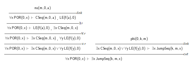
Refer to caption

Figure 4: Prooftool output of the base case proof.

Similarly, with the sequence of commands below we can output the step case proof in prooftool, see Figure 5.

scala> val step = GradedStrictMonotoneSequenceSchema.omegaSc
scala> prooftool( step )

Refer to caption

Figure 5: Prooftool output of the step case proof.

Note that to obtain the proof schema from Example 20 we have to instantiate the parameter kk with 00. In fact, we can instantiate the proof schema GradedStrictMonotoneSequenceSchema with an arbitrary value for parameters nn and mm (having kk fixed). The sequence of commands below instantiates the proof schema with the value n=2n=2 and m=1m=1.

scala> val proof1 = instantiateProof.Instantiate( le"omega (s (s 0))
                    0 (s 0) " )
scala> prooftool( proof1 )

Note that for this command it is important to import the context ctx of GradedStrictMonotoneSequenceSchema as well! We will not show the output of prooftool here, as the proof is too large to be displayed. Instead, we will output the so-called sunburst view of the proof. The sunburst view is accessible via prooftool and was introduced to obtain a means of displaying very large proofs. It can be interpreted as a structure which can be unrolled to a proof in tree-like structure. Indeed, the point in the middle of the sunburst corresponds to the end-sequent of a proof in tree-like structure. The different colors represent different types of inferences. Cut rules are displayed in green, structural rules and axioms are displayed in gray, the orange parts correspond to unary logical rules, the yellow ones to binary logical rules, strong quantifier rules are displayed in red and weak quantifier rules in blue. The sunburst of proof1 is illustrated in Figure 6.

Refer to caption

Figure 6: Sunburst output of GradedStrictMonotoneSequenceSchema for parameter n=2n=2 and m=1m=1 (k=0k=0).

The sunburst view of the instantiated proof schema for n=4n=4 and m=3m=3 is displayed in Figure 7, we obtain it with the sequence of commands below.

scala> val proof2 = instantiateProof.Instantiate( le"omega
                    (s (s (s (s 0)))) 0 (s (s (s 0))) " )
scala> prooftool( proof2 )

Refer to caption

Figure 7: Sunburst output of GradedStrictMonotoneSequenceSchema for parameter n=4n=4 and m=3m=3.

Instantiated proof schemata are essentially LK-proofs extended with an equational theory and thus, any of the proof analytic tools and methods of Gapt can be applied. The command

scala> val cs = CharacteristicClauseSet(StructCreators.extract(
                proof2))

constructs an instance of the clause representation of the characteristic NNF formula (the running example in this work). It can be also displayed in prooftool. It is also possible to construct a resolution refutation from cs using the command

scala> val res = SPASS.extendToManySortedViaErasure.getResolution
                 Proof( cs )
scala> prooftool( res )

The output is illustrated in Figure 8.

Refer to caption

Figure 8: The resolution refutation of the characteristic formula schema of the GradedStrictMonotoneSequenceSchema for parameter n=4n=4 and m=3m=3.

Moreover, we can extract an expansion proof from the resolution refutation and output it in prooftool with the sequence of commands below.

scala> val ep = ResolutionToExpansionProof( res.get )
scala> prooftool( ep )

The output in prooftool is illustrated in Figure 9.

Refer to caption

Figure 9: Expansion proof of the resolution refutation of GradedStrictMonotoneSequenceSchema for parameter n=4n=4 and m=3m=3.

There are also tools specifically designed for uninstantiated proof schemata. One of the most interesting benefits of the interactive features of Gapt is the representation of the cut-structure of a proof schema as an inductive definition. The sequence of commands

scala> val SCS = SchematicStruct( "omega" ).getOrElse( Map() )

stores the SchematicStruct in SCS. Given its type it is not possible to display it in prooftool. With the code

  val SCS: Map[CLS, ( Struct, Set[Var] )] = SchematicStruct(
           "phi" ).getOrElse( Map() )

  val CFPRP = CharFormPRP( SCS )

  CharFormPRP.PR( CFPRN )

the schematic characteristic formula is stored in CFPRP and the primitive recursive definitions of the formula is constructed with CharFormPRP.PR(CFPRP).

8 Future Work and Applications

The initial intention of this research was to develop a schematic resolution calculus and thus allowing interactive proof analysis using CERES-like methods [3] in the presence of induction. More precisely, the resolution calculus introduced in this work will provide the basis for a schematic CERES method more expressive than the methods proposed in [10, 14]. As already indicated, the key to proof analysis using CERES lies in the fact that it provides a bridge between automated deduction and proof theory. In the schematic setting a bridge has been provided [10, 14], and the formalism presented here provides a setting to study automated theorem proving for schematic first-order logic.

Our recursive semantics (Section 5) separates local resolution derivations from the global “shape” of the refutation, an essential characteristic of induction. While constructing a recursive resolution refutation for a recursive unsatisfiable formula is incomplete, it is not clear whether the problem remains incomplete when the call graph is fixed. In other words, we may instead ask: “Is providing a recursive resolution refutation, with respect to a given call graph, for recursive formulas complete?” The answer to this question is not so clear in that it depends on the resolution calculus itself as well as the associated unification problem. Both concepts are developed in this paper.

Concerning the resolution calculus presented in Section 4, both the Andrew’s calculus-like sequent rules and the introduction of global variables provide the necessary extensions to resolution accommodating the recursive nature of our formula. The unification problem discussed in Section 3 has not been addressed so far, and furthermore it may have interesting decidable fragments impacting schematic proof analysis as well as other fields.

Overall, the avenues we leave for future investigations provide ample opportunities for studying schematic theorem proving.

References

  • [1] Andrews, P.B.: Resolution in type theory. J. Symb. Log. 36(3), 414–432 (1971)
  • [2] Aravantinos, V., Echenim, M., Peltier, N.: A resolution calculus for first-order schemata. Fundamenta Informaticae (2013)
  • [3] Baaz, M., Hetzl, S., Leitsch, A., Richter, C., Spohr, H.: Ceres: An analysis of Fürstenberg’s proof of the infinity of primes. Theoretical Computer Science 403(2-3), 160–175 (Aug 2008). https://doi.org/10.1016/j.tcs.2008.02.043, http://dx.doi.org/10.1016/j.tcs.2008.02.043
  • [4] Baaz, M., Hetzl, S., Leitsch, A., Richter, C., Spohr, H.: CERES: an analysis of fürstenberg’s proof of the infinity of primes. Theor. Comput. Sci. 403(2-3), 160–175 (2008)
  • [5] Baaz, M., Leitsch, A.: Cut-elimination and redundancy-elimination by resolution. Journal of Symbolic Computation 29, 149–176 (2000)
  • [6] Brotherston, J.: Cyclic proofs for first-order logic with inductive definitions. In: Tableaux’05, Lecture Notes in Comp. Sci., vol. 3702, pp. 78–92 (2005)
  • [7] Brotherston, J., Simpson, A.: Sequent calculi for induction and infinite descent. Journal of Logic and Computation 21(6), 1177–1216 (2010)
  • [8] Cerna, D.M., Leitsch, A.: Schematic cut elimination and the ordered pigeonhole principle. In: Automated Reasoning - 8th International Joint Conference, IJCAR 2016, Coimbra, Portugal, June 27 - July 2, 2016, Proceedings. pp. 241–256 (2016), peer Reviewed
  • [9] Dunchev, C., Leitsch, A., Libal, T., Riener, M., Rukhaia, M., Weller, D., Woltzenlogel-Paleo, B.: Prooftool: a gui for the gapt framework. arXiv preprint arXiv:1307.1942 (2013)
  • [10] Dunchev, C., Leitsch, A., Rukhaia, M., Weller, D.: Cut-elimination and proof schemata. In: TbiLLC. Lecture Notes in Computer Science, vol. 8984, pp. 117–136. Springer (2013)
  • [11] Ebner, G., Hetzl, S., Reis, G., Riener, M., Wolfsteiner, S., Zivota, S.: System description: Gapt 2.0. In: International Joint Conference on Automated Reasoning. pp. 293–301. Springer (2016)
  • [12] Hetzl, S., Leitsch, A., Weller, D., Paleo, B.W.: Herbrand sequent extraction. In: Intelligent Computer Mathematics. pp. 462–477. Springer (2008)
  • [13] Kersani, A.: Preuves par induction dans le calcul de superposition. (Induction proof in superposition calculus). Ph.D. thesis, Grenoble Alpes University, France (2014), https://tel.archives-ouvertes.fr/tel-01551801
  • [14] Leitsch, A., Peltier, N., Weller, D.: CERES for first-order schemata. J. Log. Comput. 27(7), 1897–1954 (2017). https://doi.org/10.1093/logcom/exx003, https://doi.org/10.1093/logcom/exx003
  • [15] Mcdowell, R., Miller, D.: Cut-elimination for a logic with definitions and induction. Theoretical Computer Science 232 (1997)
  • [16] Schnorr, C.: Rekursive Funktionen und ihre Komplexität. B. G. Teubner Stuttgart (1974)
  • [17] Takeuti, G.: Proof Theory, Studies in logic and the foundations of mathematics, vol. 81. American Elsevier Pub. (1975)