Disclosing connections between black holes and naked singularities: Horizon remnants, Killing throats and bottlenecks
Abstract
We study the properties of black holes and naked singularities by considering stationary observers and light surfaces in Kerr spacetimes. We reconsider the notion of Killing horizons from a special perspective by exploring the entire family of Kerr metrics. To this end, we introduce the concepts of extended plane, Killing throats and bottlenecks for weak (slowly spinning) naked singularities. Killing bottlenecks (or horizon remnants in analogy with the corresponding definition of throats in black holes) are restrictions of the Killing throats appearing in special classes of slowly spinning naked singularities. Killing bottlenecks appear in association with the concept of pre-horizon regime introduced in de-Felice1-frirdtforstati; de-Felice-first-Kerr. In the extended plane of the Kerr spacetime, we introduce particular sets, metric bundles, of metric tensors which allow us to reinterpret the concept of horizon and to find connections between black holes and naked singularities throughout the horizons. To evaluate the effects of frame-dragging on the formation and structure of Killing bottlenecks and horizons in the extended plane, we consider also the Kerr-Newman and the Reissner–Norström spacetimes. We argue that these results might be significant for the comprehension of processes that lead to the formation and eventually destruction of Killing horizons.
August 11, 2026
I Introduction
One of the most important exact solutions of Einstein vacuum field equations is the Kerr metric, which in Boyer-Lindquist (BL) coordinates can be expressed as
| (1) | |||
| (2) |
It describes an axisymmetric, stationary, asymptotically flat spacetime. The parameter is interpreted as the mass of the gravitational source, while the rotation parameter (spin) is the specific angular momentum, and is the total angular momentum of the source. The spherically symmetric (static) Schwarzschild solution corresponds to the limiting case with . If the spin-mass ratio is within the range , the spacetime corresponds to a Kerr black hole (BH). The extreme black hole case is defined by the relation , whereas a super-spinner Kerr compact object or a naked singularity (NS) geometry occurs when .
The Kerr metric tensor (1) has several remarkably properties.
(i) The metric (1) is invariant under the application of any two different transformations of the form where is one of the coordinates or the metric parameter : a single transformation leads to a spacetime with an opposite rotation with respect to the unchanged metric.
(ii) The Kerr solution is stationary and axisymmetric due to the presence of the Killing fields and , respectively.
An observer moving with uniform angular velocity along the curves constant and constant will see a spacetime which does not change at all (therefore, the covariant components and of the particle four--momentum are conserved along the circular geodesics).11 1 We use geometrical units with and the signature , Greek indices run in . The four-velocity satisfies the condition . The radius has units of mass , and the angular momentum units of , the velocities and with and . For the sake of convenience, we consider a dimensionless energy and an angular momentum per unit of mass .
(iii) As the metric is invariant under reflections with respect to the equatorial hyperplane , equatorial trajectories are confined in the equatorial geodesic plane.
For black hole and extreme black hole spacetimes, the radii
| (3) |
solutions of , are the radii of the outer and inner Killing horizons, whereas
| (4) |
solutions of , are the outer and inner ergosurfaces, respectively, with . In an extreme BH geometry, the horizons coincide, , and the relation is valid on the rotational axis (i.e., when ). In the Kerr BH spacetime, the Killing vector representing time translations at infinity, , becomes null on the outer ergosurface, , which is, however, a timelike surface. On the contrary, a Killing horizon is a lightlike hypersurface (generated by the flow of a Killing vector) on which the norm of a Killing vector vanishes. That is, the Kerr horizons are null surfaces, , whose null generators coincide with the orbits of an one-parameter group of isometries, i.e., in general there exists a Killing field , which is normal to .
Some additional properties of the Kerr spacetime include:
(iv) In the limiting case of the Schwarzschild spacetime (), is the Killing horizon with respect to the Killing vector . In general, in the special case of static (and spherically symmetric) BH spacetimes, the event, apparent, and Killing horizons with respect to the Killing field coincide.
(v) The event horizons of a spinning BH are Killing horizons with respect to the Killing field , where is the angular velocity of the horizon.
In this work, we extensively discuss the properties of the Killing vector in the case of NS geometries. In BH spacetimes, this vector plays a crucial role in defining thermodynamic variables. As we will see below, the velocity (and its limit ) and the vector (and its limit ) are important for defining horizons and establishing relations between black holes and extreme black holes. In fact, it can be shown that: (a) In the context of the rigidity theorem, represents the BH rigid rotation. Stated differently, the (strong) rigidity theorem connects the event horizon with a Killing horizon. In fact, under certain conditions, the event horizon of a stationary asymptotically flat solution (with matter satisfying suitable hyperbolic equations) is a Killing horizon. (b) The BH event horizon of this stationary solution is moreover a Killing horizon with constant surface gravity (zeroth BH law-area theorem– the surface gravity is constant on the horizon of stationary black holes) Chrusciel:2012jk; Wald:1999xu. (c) Finally, the surface area of the BH event horizon is non-decreasing in time, which is the content of the second BH law (the laws state also the impossibility to achieve by a physical process a BH state with surface gravity .)
We note here that the surface gravity of a BH may be defined as the rate at which the norm of the Killing vector vanishes from the outside. (The surface gravity is related to the acceleration of a particle corotating with the BH at the horizon and it can be written as (). It is, therefore, a conformal invariant of the metric).
Possibly, we could isolate the contribution of the rotation in the expression of the surface gravity by comparing it with the static (and spherically symmetric) metric of Schwarzschild. In fact, the Kerr BH surface gravity can be written as the combination , where is the Schwarzschild surface gravity, while is the contribution due to the additional component of the BH intrinsic spin; is, therefore, the angular velocity (in units of ) on the event horizon.
These laws, which depend also on the horizon angular velocity, impose important constraints on any physical process in the BH spacetime, but they also allow to distinguish the static solution, , from the Kerr BH solution. The first law of BH thermodynamics, applied to a Kerr BH spacetime, actually relates the variation of the BH mass, horizon area and angular momentum, including the surface gravity and angular velocity on the horizon, i.e., . In here, the term dependent on the BH angular velocity represents the “work term” of the first law, while the fact that the surface gravity is constant on the BH horizon, together with other considerations, allows us to associate it with the concept of temperature. This aspect tends to emphasize the difference (also topological) between Kerr’s BH and its extreme solution: in the extreme case, where (), it is easy to see that the surface gravity is zero and, considering the association with the temperature, there is , with consequences also with respect to the stability against Hawking radiation. Nevertheless, the entropy (or BH area) of an extremal BH is not nullChrusciel:2012jk; Wald:1999xu; WW; Li:2013sea; Jacobson:2010iu; Sha-teu91; Goswami:2005fu; ze. (An analogue implication of the third law it is said that a non-extremal BH cannot reach an extremal case in a finite number of steps.)
We investigate the properties of Kerr BHs and NSs from the point of view of stationary observers. In particular, we explore the characteristics of light surfaces, which correspond to the limiting frequencies of stationary observers. From the analysis of these orbital frequencies (and associated orbits), we introduce the concept of Killing throats, arising in NS spacetimes as the “opening” and disappearance of Killing horizons. More precisely, the Killing throat is a region bounded by a particular set of curves that we identify with the frequency of a stationary observer, which depends on the radial distance and the spin parameter of the source. We define a Killing bottleneck as a particular case of a of Killing throat that appears in weak naked singularities (WNS). Thus, bottlenecks can be interpreted as throats “restrictions" that characterize WNS . The concept of strong and weak NSs depends on the value of the spin parameter and has been explored in several works Pugliese:2010he; Pu:Kerr; Pu:Neutral; Pu:Charged; Pu:KN; ergon; Pu:class; observers. However, in general, they are also differently defined as strong curvature singularities, for example, in strong. Regarding various NSs properties and characteristics of the gravitational collapse, possible formation and stability of naked singularities as well as other analysis concerning observational phenomena related to possible NSs existence, we refer also to Bini; deFelice; FDEFELICE1; Chakraborty:2016mhx; Blaschke:2016uyo; Bejger:2012yb; Stuchlik:2004wk; Stuchlik:2012zza; Nakao:2017rgv; Gao:2012ca; Evo; Pradhan:2012yx; Kolos:2013bca; Stuchlik:2010zz; Esitenza; Joshi-Book; Giacomazzo:2011cv; miller; Wald:1991zz. In this work, WNSs are characterized by spin-mass ratios close to the value of the extreme BH. To explore these NS effects and to compare BHs with NSs, it is convenient to introduce the concept of “metric bundles” and “extended planes”. A metric bundle is a curve on the extended plane, i.e., a family of spacetimes defined by one characteristic photon orbital frequency and characterized by a particular relation between the metrics parameters. This turns out to establish a relation between BHs and NSs in the extended plane. All the metric bundles are tangent to the horizon curve in the extended plane. Then, the horizon curve emerges as the envelope surface of the set of metric bundles. As a consequence, WNSs turn out to be related to a part of the inner horizon, whereas strong naked singularities (SNSs) with are related to the outer horizon.
This work is organized as follows. In Sec. (II), we study the main definitions and properties of stationary observers and light surfaces in BH and NS Kerr geometries. Killing throats and bottlenecks are the focus of Sec. (III). In Sec. (IV), we introduce the concept of metric bundles and discuss the resulting connections between BHs and NSs. These results are generalized to include the cases of the Kerr-Newman and Reissner-Nordström spacetimes in Sec.(V). Concluding remarks and future perspectives follow in Sec. (VI). This article closes with two Appendices. The off-equatorial case in the Kerr and Kerr-Newman geometries is considered in Appendix A. In Appendix B, we study the areas of the horizons and regions of the extended plane delimited by different metric bundles. Throughout this work, we introduce a considerable number of symbols and notations which are necessary to explain all the details of the results we will obtain. For clarity, we list in Table 1 the main symbols and their definitions.
| limiting frequencies for stationary observers: Eqs.(7)-(8) | |
| limiting frequency at the singularity and frequency of the metric bundle: Eq. (9)-Sec. (IV) | |
| null Killing vector (generators of Killing event horizons): Eq. (10) | |
| light surfaces radii: Eq. (11) | |
| frequencies at the horizons : Eq. (12) | |
| photon orbits with frequencies at the horizons: Eq. (13)–Fig. 1 | |
| metric bundles in the extended plane : Sec. (IV) | |
| in terms of the bundle frequency : Eq. (15) | |
| horizon curve in the extended plane: Fig. (8) | |
| closing radii of the metric bundle in (= for ): Eq. (16) | |
| spin of metric bundle tangent to the horizons in : Eq. (17)– Fig. (13) | |
| bundle origin, i.e., with : Figs. 14, 15, 16; Tables 3 and 2 | |
| horizons relations I | , , |
| (, ): Fig. (13) | |
| horizons relations II | , , (), where and : Fig. 14 |
| SNS | (=) strong naked singularities , for |
| for : Fig. (13) | |
| WNS | weak naked singularities : Fig. (13) |
| for , and for : Fig. (13) | |
| Left region Fig. (13) | |
| Right regionFig. (13) | |
| up-sector Fig. (13) | |
| down-sector Fig. (13) | |
| second frequency of a metric bundle: Eq. (22) | |
| metric bundles parameterized for the tangent point : Eq. (23) | |
| tangent curve to the horizon in terms of : Eq. (24) | |
| solution of the tangency condition : Eq. (25), Fig. (17) | |
| metric bundles in terms of the charge : Eq. (35) |
II Stationary observers and light surfaces
Stationary observers have a tangent vector which is a spacetime Killing vector; their four-velocity is, therefore, a linear combination of the two Killing vectors and as:
| (5) | |||
| (6) |
where (a dimensionless quantity) is the (uniform) angular velocity, while is a normalization factor ().
Because of the symmetries, the coordinates and of a stationary observer are constants along its worldline, consequently a stationary observer does not see the spacetime changing along its trajectory. Timelike stationary observers have angular velocity bounded in the range
| (7) | |||
()22 2 This equation corrects a typo in Eq. (8) of Ref. observers. Zero Angular Momentum Observers (ZAMOs) are defined by the condition and have angular velocities , which depend on the spin. A ZAMO, well defined in the ergoregion, corotates with the BH. ZAMOs have interesting properties in the case of slowly spinning naked singularities and certainly offer a particularly appropriate and convenient description of the spacetime in the ergoregion –see for example observers; ergon and Gariel:2014ara; Pelavas:2000za; Herdeiro:2014jaa; Cardoso:2007az; CoSch; Frolov:2014dta; Stu80; CCQ-suer; Schee:2013bya; Torok:2005ct; BiStuBa89; Patil; erg1. Static observers are defined by the limiting condition and cannot exist in the ergoregion. The particular frequencies provide an alternative definition of the horizons. Since the horizons are null surfaces, it should hold that , which is the limiting angular velocity for physical observers corresponding in fact to orbital photon frequencies. The quantity in parenthesis in the r.h.s. of Eq. (6) becomes null for photon-like particles and the rotational frequencies , as in Eq. (7). On the equatorial plane, the limiting orbital frequencies are
| (8) |
The following limits are valid
| (9) |
The limit is used to formally explore the behavior in the strong NS singularity regime, for a given constant value of , and more generally in the limit . As already mentioned in Sec. (I), the Killing vector
| (10) |
can be read as generator of null curves () as the Killing vectors , null at r = , are also generators of Killing event horizons.
III Killing throats and bottlenecks
The concept of Killing throats emerges through the analysis of the radii (the frequencies ) with respect to the orbital frequency (the radius ) of light-like particles – see Figs. 2 and 3. A Killing throat in NS geometries is a connected region in the plane, which is bounded by or equivalently , and contains all the stationary observers allowed within the limiting frequencies . Conversely, a BH Killing throat is either a disconnected region in the Kerr spacetime (in a sense similar to the concept of a path-connected space) or a region bounded by non-regular surfaces in the extreme Kerr BH spacetime. A Killing bottleneck in a NS spacetime is a narrowing of the Killing throat which appears only for specific naked singularities and involves a narrow range of frequencies and orbits–Figs (1). The limiting case of a Killing bottleneck occurs in the extreme Kerr spacetime, as seen in the BL frame, where the narrowing actually closes33 3 Killing throats and bottlenecks, represented Figs (1) and (2), were grouped in Tanatarov:2016mcs in structures named “whale diagrams”, considering the escape cones, particles motion and collisionals problems in the Kerr and Kerr-Newman spacetimes–see also Mukherjee:2018cbu; Zaslavskii:2018kix. at the BH horizon .
More generally, the Kerr horizons determine the following frequencies:
| (12) |
It should be noted then that while the horizons radii are functions of the metric parameters only, meaning that there is only one frequency, , on the horizons , respectively, the Killing bottlenecks depend on both frequency and radius, corresponding to the fact that the throat never closes, but in the limit of the extreme Kerr spacetime.
Considering again the horizons frequencies , we introduce the radii representing the set of photon orbits with frequencies at the BH horizons
| (13) | |||
| (14) |
with – see Fig. 1. In Sec. IV, this property is displayed in a different context, showing a close connection between BHs and NSs. Moreover, the Killing horizons, , are defined as the tangent (envelope surfaces) of the curves defined by the conditions constant.


The existence of implies that an observer could eventually measure the frequency of the outer horizon on the equatorial plane, while no information can be obtained from for the inner horizon frequency . In this sense, we may call this property as inner horizon confinement. This situation can be used to distinguish between slow rotating BHs and fast spinning BHs since the distance decreases with the spin. The existence of these radii may be related to the bottleneck presence.
Figure 2 shows the formation of the Killing throat as the spin of the naked singularity varies. The emergence of the Killing bottleneck in terms of the frequency ( plane) and of the radius ( plane) is evident in the case of weak naked singularities, i.e., slow spinning singularities. We specify below the limiting spin values which define weak naked singularities.

 |

 |
 |
To evaluate the effects of the spacetime dragging on the formation of a Killing bottleneck, we investigate in Sec. (V) the Kerr-Newman geometry, the limiting static case of the Reissner Nordström geometry, and the off-equatorial case.
Three distinct phases are significant in the process of formation of bottlenecks:
(1) Coalescence of the Killing horizons, which occurs in the extreme Kerr BH solution;
(2) Formation of the Killing throat and emergence of the bottleneck in weak NSs;
(3) Disappearance of the Killing bottleneck in strong NSs.
The analysis carried out in Figs. 2 and 5 suggests that the Killing bottlenecks can be defined through the conditions and . On the other hand, the radii and, analogously, characterize the curvatures of the curves and .
Killing bottlenecks, identified in observers as ripples in the plane (see Figs. 3 and 4), were interpreted in the BL frame as “remnants” of the disconnection between the Killing throat present in BH-geometries and the singular bottleneck of the extreme BH.
 

 |
  |


The radii and the frequencies , as shown in Fig. 5, define closed and limited surfaces. This implies that a Killing throat can always exist, but a Killing bottleneck appears only for certain frequencies and values of the dimensionless spin . In fact, is defined for NSs with spin , where . On the other hand, and are not closed and tends to the horizon frequency for very small spins. This means that the Killing bottleneck actually survives only for , where, at . However, the bottleneck frequencies satisfy the inequalities . Increasing the spin , at constant mass, a bending of the frequency appears44 4 Note that the Killing bottleneck and Killing throat inherit some of the properties of the Killing vectors, particularly, regarding conformal transformations of the metric or vectors. Consider a Killing throat defined by two Killing vectors . The linear combination defines a Killing vector and we can define a Killing field up to a conformal transformation. In other words, identifies a Killing throat up to a conformal transformation. The simplest case is when one considers a conformal expanded (or contracted) spacetime where . This holds also for a conformal expanded Killing tensor . .
There are several notable radii associated with the frequencies and light surfaces , which are related to the extremes and saddle points of the curves in the region (see observers). The function is considered in Figs. 6 and 7. The radius , solution of , clearly shows the presence of closed surfaces for and , and provides a characterization of the Killing bottleneck. An analysis of and in Figs. 6 and 7 shows the emergence of horizons as the envelope surface in the plane of the limiting frequencies . This important aspect will be addressed in details in Sec. IV, revealing the role played by the Killing horizons in BHs-NSs connections.


 |

 |
IV Unveiling BHs–NSs connections
In this section, we explore the entire parameterized family of Kerr solutions with . To this end, we introduce the concept of extended plane , where the entire collection of metrics of a parametrized family of solutions can be considered.
We may say that a quantity in the plane induces a realization of the extended plane, where is a parameter that characterizes the entire family of solutions. For the case considered in this work, is the dimensionless spin parameter. A special and simple example of an extended plane realization is given in Fig. 8, where we investigate constant frequency surfaces defining families of spacetime geometries that we call “metric-bundles”, , labeled by a frequency parameter constant. Such definitions are set from the properties of stationary observes and their limiting frequencies . In the extended plane, naked singularities and black holes can belong to the same metric bundle. In the extended plane of Fig. 8, BHs horizons correspond to the spin-curve ; we shall see that in such a plane the BHs horizons define properties for all possible Kerr geometries, including BHs and NSs, that unveil an interesting connection between BHs and NSs.
Metric bundles
Here, we specify the idea of metric bundles for the Kerr family of solutions. Solving Eq. (8) for the spin , we obtain the following two quantities
| (15) |
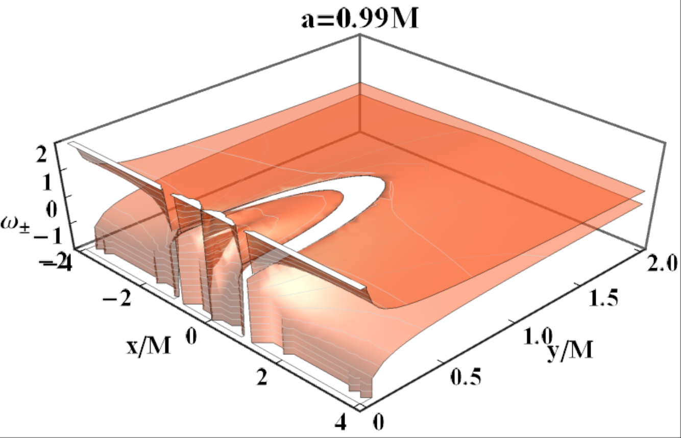
which are plotted in Figs 8 and 9 as functions of , for different values of the frequency . Note that in the region , negative orbital frequencies are possible because they are associated to the retrograde (counterrotating) motion with respect to the central object; this fact implies the possibility of negative values of for –see Figs. 8. However, in this section, we restrict our analysis to the ergoregion , where and –see Figs. 8 and 9. Each spacetime of the Kerr family is represented (restricted to the equatorial plane) in the extended plane of Fig. 8 by a constant surface constant (horizontal lines in Fig. 8).
The metric bundles are defined by the curves of constant frequency in – Fig. 8. Each for a fixed frequency is represented by closed and bounded curves which are continuous almost everywhere in . Below, we will discuss extensively the properties of these curves.
The bundles contain an (almost) continuum and infinite set of metric parameter values . Each value of sets a specific Kerr geometry. From Fig. 8, it is clear that eventually some bundles contain both BHs and NSs spacetimes, others define only BHs, while none of the bundle is constituted by NS only. In fact, all the metric bundles are tangent at least in one point to the horizons . Thus, from the quantities (15) an alternative definition of BHs Killing horizons emerge. Indeed, from Fig. 8, it follows that the horizons arise as the envelope surfaces of the curves , i.e., the metric bundles in . This will be a crucial property of the metric bundles with significant consequences that allow us to connect NSs to BHs in the extended plane. In fact, since the curve is tangent to all metric bundles , the (inner and outer) horizons contain all the frequencies defining each metric bundle and, therefore, describing both NSs and BHs in the extended plane.

 |
 |


 |
From Fig. 8, it follows that a metric bundle has its origin on the vertical axis of and closes on the tangent point to . The closeness of the metric bundles is due to the spacetime rotation. To investigate the solutions (15), which define the closed bundles, we solve the condition and find
| (16) | |||
The frequency of Eq. (16) is a solution of the equation (see Fig. 10); the function is, therefore, the frequency associated to the orbits , where defines the metric bundle. In fact, does not depend on the spacetime spin because the information on the corresponding geometry can be extracted from through , i.e., from the condition . Consequently, is a function of the radius . The pairs identify the corresponding spin origin (also origin of the metric bundle), which is defined by the frequencies and at –Fig. 10. Asymptotically, for very large values of , the value is approached as shown in Fig. 8, where is valid on the line , that is, approaching the limiting geometry of the static and spherically symmetric Schwarzschild spacetime.
We note that is negative for positive values of the frequency. As we are restricting our analysis in this work to the case , we shall not consider ; nevertheless, an analysis of the case would, in fact, provide additional information about the spacetime structure even in the equatorial plane. A very small , on the other hand, corresponds to a very large (origin) spin . Note that the spin corresponds to the frequency , which was introduced in Eq. (8) by considering the behavior of the stationary observer frequencies near the singularity ; this is of importance in NS geometries as described in Sec. III. The properties of this special frequency have also been extensively discussed in observers. More generally, as noted in Secs. II and III, the dimensionless spin parameter is related to the quantity though the frequencies of the light surfaces (see observers). Then, the function in Eq. (16) is obtained as . As shown in Fig. 10, the condition is valid only at the spacetime singularity ; otherwise, , while the condition (a NS) is reached asymptotically for large values of .
Note that the asymptotic limit of is relevant as it corresponds to a metric bundle at constant frequency , which defines the point of the envelope corresponding to the extreme Kerr BH solution . Figure 12 refers to the analysis of Fig. 8 and sketch the correspondence between BHs and NSs derived from the analysis of . The envelope of the curves is defined as the set of points for which , i.e., as the curve tangent to all or also as the boundary of the region filled by the curves . Then, small changes of and shifts along the orbit radius leave almost constant as are continuum functions.
The relation between the radius , the spin and frequencies has to be confronted with Eq. (12) for the frequencies at the horizons and radii of the BH Killing horizons. These quantities play an important role also for the Killing bottleneck emergence considered in Sec. III, as the surfaces constant are related to the solutions of Eq. (8) and shown in Fig. (11). The relation of Eq. (16) is also used in Fig. 12 to unveil some BHs and NSs properties: The points on the lines constant for lead to the Killing bottleneck emergence of Fig. 11.
BHs and NSs in metric bundles
As discussed above, a metric bundle can comprise only BHs or BHs and NSs. Moreover, the horizons describe BHs and NSs in the extended plane. In the remaining of this section, we describe this last aspect and the BHs-NSs relation more closely.
Firstly, Fig. 10-left represents BHs and NSs in the plane. The plane is divided into regions, where the metric bundles include BHs or NSs; there are regions with only BHs or NSs and transition regions that cross different sections and are connected to Killing horizons and bottlenecks–see also Fig. 11. A special transition region is, for example, around the extreme BH horizon with frequency value , which corresponds to the extreme Kerr BH.
We concentrate on the restricted plane determined by in Figs. 8. The restriction of the extended plane to exploits the symmetry by reflection around the axis , where negative origins of metric bundles build up the horizons . The plane has the following remarkable sections: , , , , and . The line includes BHs and NSs. represents the collection of all origins . A variation of the dimensionless spin of the singularity (at ) corresponds to a variation of in . This line also represents the singularity frequencies . Moreover, we define and the set for the Killing horizons. Curves at constant closes on and have origins in . The line describes the limiting case of the Schwarzschild solution. crosses in and . Finally, the set describes the extreme Kerr spacetime and crosses at and . The collection of all the points constant generates the light-curves shown in Fig. 11, where the Killing bottleneck and Killing throat emerge at .
According to Fig. 8, metric bundles can be classified in two classes. (1) The first class includes the curves tangent to , including those bundles which are “entirely” contained in the BH sector of , i.e., and . (2) The second class includes metric bundles tangent to the outer horizon , containing BHs and NSs in the same bundle. These two classes are separated by the limiting bundle with origin and tangent to the maximum of ; that is, the point in with , for and frequency , describing the extreme Kerr spacetime. Bundles with origins in the BH sector are completely contained in an “inaccessible” region between the singularity, , and the inner horizon . Bundles with origin in the the naked singularity sector comprise BH and NS geometries, which are, therefore, related because they are contained in the same metric bundle. (Notice that the definition of , through the stationary observes definition, provides a BH-NS relation). The case of very strong NSs (very large , asymptotic value ) corresponds to the limiting point and –see Fig. 8. This suggests that the NS sector is closely related to the BH sector. We explore this connection more deeply below.

 |
The horizons as an envelope surface of the metric bundles
An important consequence of the approach presented here is that it allows us to establish a relation between BHs and NSs. In fact, the outer horizon in emerges as an envelope surface of metric bundles with only NSs origins. That is, the BH outer Killing horizon relates a BH with with a NS with .


 |
The inner horizon in can be constructed by metric bundles with NS and BH origins. Viceversa, the BH horizons are tangent to all the metric bundles. All the BHs and NSs frequencies are, therefore, related to the horizon frequency , and all horizon frequencies are the limiting orbital photon frequencies in NS and BH spacetimes–Figs (8). As the horizon is tangent to all the metric bundles, each metric bundle is defined by one frequency , which coincides with the horizon frequency on the tangent point in the extended plane. Frequencies in (15) are actually the limiting frequencies . It follows that the metric bundles, connected the singularities frequencies , are defined by the origins of the metric bundles and the horizon frequencies .
Remarkably, the construction of the inner horizon is confined to metric bundles contained entirely in the BH sector. This fact could lead to important consequences, when considering the collapse towards a BH and the process of formation of the inner horizon. These metric bundles are all confined in the region and . This implies that the inner horizon of a BH with spin is related to a metric bundle with origin in the BH or WNS () regions, while the outer horizon is related to a NS metric bundle.
Before continuing, it is convenient to return to the concept of metric bundle, as shown in Fig. 8, and analyze three particular curves in detail: (1) the horizontal lines constant of ; (2) the vertical lines constant and; (3) the curves corresponding to horizons.
(1) The horizontal lines =constant
For a BH or a NS with , there are two curves of the bundle, which are tangent at a point on the horizons. Each metric bundle is associated to a constant frequency, , defined by the bundle origin . Considering a bundle, there is a pair of points and with constant and , which are located respectively on the two curves of the bundle. A special case is the pair of points present on the origin line, , where . Also the horizons for the extreme Kerr spacetime are special. Note that, in general, the condition on the horizon for leads to Eq. (13). On the orbits , light-like orbital frequencies are equal to , where . There are two special geometries associated to the closure points and : represents the singularity with , corresponding to a spacetime with spin . Moreover, the second special geometry is always a BH, whose (inner or outer) horizon has the frequency , i.e., the frequency of the bundle. We investigate the spin of this specific spacetime below.
We note that metric bundles cross each other in . This means that, in a fixed spacetime with a fixed radius, there are two limiting frequency values . Therefore, the maximum number of crossing points between metric bundles is two. Consequently, there are two crossing metric bundles with origins at , respectively.
(2) Vertical lines constant.
Let us now focus on the vertical lines in and the intersections on each metric bundle. For a fixed orbit , there are, in general, two Kerr geometries corresponding to the spins of the same bundle. In addition, there are the following limiting cases: 1. At there is an infinite number of origins, where on a bundle. 2. The point is the tangent point of the vertical line to the bundle, satisfying the condition – see Eq. (16) and Fig. 10. The condition is satisfied only in special geometries . In general, for , there are two geometries , corresponding to two BHs or one BH and one NS. This implies that at a fixed , there are two geometries with frequencies . The case of the geometries identified in the extended plane by the vertical lines will be clarified at the end of this section because it is necessary to consider the tangency conditions as shown in Fig. 17. With respect to this property, , there are two exceptions represented by the metric bundles with vertical lines tangent to the horizon. There are two asymptotic cases, where ; these cases with respect to the horizon points and () correspond to the limit of the Schwarzschild spacetime– Fig. 17. In general, a vertical line on a metric bundle defines two geometries with and . More details on this point will be addressed at the end of this section. In other words, this property relates limiting frequencies of different spacetimes. This result is in agreement also with the results presented in Sec. III.
(3) The horizon surfaces
All the metric bundles have the frequencies at the horizon in the extended plane. As the metric bundle frequency is also a limiting photon orbital frequency or and as all frequencies represent also the horizon frequency , then the limiting photon frequencies on an orbit in all the spacetimes are the horizons frequencies in the extended plane. Viceversa, the set of the horizon frequencies in the extended plane is the collection of all the limiting orbital photon frequencies in any BH or NS spacetime. This issue will be discussed in detail below.
BHs-NSs correspondence
The relation between BHs and NSs can be formalized by introducing the functions and of the origin as follows
| (17) | |||
| (18) |
The behavior of these functions is plotted in Figs. 13. For a fixed value of the origin , the function defines univocally the outer or the inner horizon. This relation includes the Schwarzschild limiting case, which corresponds to the limit , and the extreme Kerr spacetime, which is connected with the naked singularity value –see also Figs. 12. More precisely, is the solution of the equations , where –while is the solution of the equations , providing information about the orbits where the curves close at the horizons. The analysis of off-equatorial and charged generalizations considered in Sec. V reaffirms this result.

According to Figs. 8, each point on the horizon is univocally related to a NS or a BH metric in the plane. Each frequency is in correspondence with a point on or . In this sense, we might say that the information contained on the horizon (the frequency ) is extracted by the functions .
Furthermore, it is immediate to see that from the expression of Eq. (17), we obtain a relation between the horizon tangent spin (horizon frequency) and the bundle origin (bundle frequency), namely, ; in particular, from , it is seen that the bundle frequencies represent all (and only) the horizon frequencies on the tangent point, i.e., . This implicitly relates also the horizons frequencies with the singularity frequencies; there are then particular BH spacetimes, where the outer horizon or the inner and outer horizon are defined by bundles with NSs. We detail this aspect below. Here we note that there is only one fixed point for the transformation , namely , and for .
We now introduce the concept of couples of related metric bundles, say, BD and BC (see Fig. 14). In the first couple, the first bundle has its origin in the NS region (tangent to the outer horizon) and the second bundle is completely or partially contained in the BH region (tangent to the inner horizon). The two bundles with origins () share equal tangent spin . That is, if , then the bundle with origin , frequency , has the contact spin in with horizon frequency . The second bundle of the couple has its origin at , frequency , tangent spin in and horizon frequency . Bundles and determine, in the sense of the envelope surface, respectively, the outer horizon and the inner horizon of the BH spacetime with spin . The relation between the tangent points and the origin and the relations between BHs and NSs through the bundles will be addressed in full details below. Importantly, the condition of the bundle correspondence, i.e., , leads to the non-trivial solution (see DD and BB model bundles of Figs. 14, 15, and 16 and Tables 3 and 2). In terms of the horizon frequency (equal to the bundles frequencies), there is ; in fact, using Eq. (12), this relation can be written in compact form as (or we can write ), which is independent of the spin , in general. In Fig. 14, the solutions correspond to and .
In the second couple, BC, the origin spin of one bundle is the tangent point of the second bundle with origin (therefore, is always a BH and the other bundles are all BHs). An example of these couples are the models BB and CC of Figs. 14, 15, and 16 and Tables 3 and 2.
To enlighten some properties of the BC and BD bundles, we consider the difference as a function of and the recurrence relation for , i.e., where . Then, decreases with the cycle order (see Fig. 14). In fact, in BC bundles, the cycles are confined to the inner horizon in the extended plane (apart from the starting point ). Naturally, the only fixed point, , of this relation is in , corresponding to the extreme BH.
Bundles BD have coincident cycles and bundles BC have partially coincident cycles; therefore, BD and BC bundles are related by partially coincident cycles (see Table 2 and Fig. 14).
| 1 (BB) | 0.8 | 0.689655 | 0.616366 | 0.562903 | 0.521586 | 0.48837 | 0.460889 |
|---|---|---|---|---|---|---|---|
| 2 (CC) | 1. | 0.8 | 0.689655 | 0.616366 | 0.562903 | 0.521586 | 0.48837 |
| 4 (DD) | 0.8 | 0.689655 | 0.616366 | 0.562903 | 0.521586 | 0.48837 | 0.460889 |
| 1/2 (AA) | 0.470588 | 0.445902 | 0.424787 | 0.406451 | 0.39033 | 0.376008 | 0.363172 |
| (1/2)=8 | 0.470588 | 0.445902 | 0.424787 | 0.406451 | 0.39033 | 0.376008 | 0.363172 |
| (1/2)=0.470588 | 0.445902 | 0.424787 | 0.406451 | 0.39033 | 0.376008 | 0.363172 | 0.351579 |

 |

 |
To conclude this analysis, we note that it is possible to find a linear relation between the horizons curves (in the extended plane) by re-expressing the curve of the inner horizon as a function of the outer horizon (on the lines costant) and, viceversa, i.e., and –Fig. 14.
BH-NS correspondence: one-to-one relation
There is a one-to-one correspondence between the points of the horizons, the horizon frequencies, and the spins for NSs or BHs. BHs are related to a part of the curve, SNSs () correspond to , and WNSs () are in correspondence with the envelope surfaces of the inner horizon, i.e., for . The limiting cases of Schwarzschild, , and extreme Kerr BH, , are connected with the limit and the double point , respectively.
In fact, we can say that , and, viceversa, there is one and only one , where is the horizon frequency, i.e., we connect points of to points of of the horizons by considering that each metric bundle relates univocally an origin of with a tangent point of . ( is solution of ). Any origin of the metric bundle , associated to a frequency constant, is associated to one and only one point or the outer , according to the origin .
A special case is the extreme Kerr BH solution, where the origin spin , associated to the metric bundle of constant frequency , crosses the horizons at and . In general, for a fixed origin , there are two frequencies and , respectively, where is the frequency of the metric bundle , and is the horizon frequency defined by the spin defined by the tangent point. .
The one-to-one BHs-NSs correspondence is described by the function as given in Eq. (17) and illustrated in Fig. (13). We can say that each BH solution is connected to one and only one in , as it emerges from the analysis of the Killing horizons and light frequencies on the equatorial plane and, viceversa, each NS is related to one BH. These considerations include the limiting cases of the Kerr extreme spacetime, where the associated metric bundle has origin , and the limiting case of the static Schwarzschild BH, which is connected to the NS with . The BH-NS relation allows us to consider a spin shift from an initial () source as corresponding to a shift of the respective (); therefore, the pair shifts to the pair . The segment of transforms into , becoming larger or smaller depending on the curve as shown in Fig.13.
To conclude this section, we analyze the relation between the tangent radius on the horizon and the bundle origin . We start with a description of Fig. 13.
Analysis of Figure 13
Figure 13 represents the spin versus . Spins and are connected through . The sectors and regions in this figure are determined by the following special boundary spins, considering that and :
the origin distinguishes NSs from BHs;
the spin defines the left region where (for BH and WNS) and right region where (for );
the spin defines the up-sector where (for ) and the down sector where (for );
the spin distinguishes strong naked singularities and .
Consequently,
a bundle origin in the BH-region corresponds through the horizon curve to singularities ();
origins in the WNS-region correspond to .
Therefore, correspond, through the tangency with the inner horizon curve , to BHWNS;
the origin in corresponds to ;
the origin in corresponds to .
Therefore, is related to .
Because , increasing the origin spin and the tangent spin increases the left region. Let us consider the BHs and NSs correspondence determined by the tangent point spin . Note that a fixed origin (down-right region) corresponds to the outer horizon tangent point (we identify ). This is sufficient for the determination of the spin and the origin of the bundle metric tangent to the inner horizon in ; therefore, this defines the inner horizon of the spacetime with spin .
Similarly, in the right-up region there are couples following related geometries : (1) and (2) .
We note that the origins () are in correspondence with a ; also the and are in correspondence with a .
Therefore, in general there is a correspondence , i.e, the origin of the bundle defines a tangent point to the horizon and or in the spacetime with ; correspondingly, there is the bundle with origin whose tangent point to the horizon is and or , respectively.
Therefore, the following triple relations hold
| (19) | |||||
| (20) |
The geometries of the triple relations given in Eq. (19) are bounded together by and the inner horizon ; on the other hand, the geometries of the two relations in Eq. (20) are bounded together by . The geometries of the last two triple relations are bounded by . The sets ((b) and (c)) and ((a) and (d)) are related by an exchange of spins , . Bundles corresponding to the tangent (same tangent point spin) belong to triplets connected by arrows. We shall see this also below considering some examples–see also Table 2.
The black hole area, delimited by the (outer) horizon, is a crucial quantity, determining the thermodynamic properties of BHs. Given the relevance of this concept, we study in Sec. (B) some properties of the areas of the regions delimited by metric bundles and compare them with the horizon area in the extended plane , i.e., the region in the plane bounded by the horizon curve .
To conclude, we show that the horizons frequency defines the bundles frequencies. We will resume part of the discussion carried out in relation with Eq. (17). We also investigate the limiting frequencies obtained from the bundles crossing and some properties of the tangents to the horizons in the extended plane.
On the frequencies
The bundle frequency is a limiting photon-like frequency, or as introduced in Sec. (II), at the point of the bundle. The second, limiting photon frequency at the point , or , respectively, is determined by the bundles crossing. As previously discussed, there is a maximum of two bundles at the intersection. This second frequency is, therefore, the solution of , where is the known frequency of the bundle , is a fixed point of the bundle. The second photon frequency , identifying the related bundle , is a function of and :
| (21) | |||||
| (22) |
The solutions for constant are shown in Fig. 15. Note that the limiting curve for the constant frequencies curves is of Eq. (16)–see also Fig.10,11.
By definition, the frequency is constant along the bundle; thus, the bundle frequency is the bundle origin frequency and, particularly, the frequency at , where is the bundle spin at the tangent point on the horizon curve. We can show that the bundle frequency coincides with the horizon frequency at the tangent point , that is, .
First, note that the bundle frequency is defined in . The analysis of the frequency variation domain gives us indications that both the inner and outer horizon frequency define the bundle frequency, as there is and (for )–see also Fig. (1). Then, condition , where is the union , leads to , relating the tangent-point-spin and the bundle origin .
Fig. 3 and Table 15 show some notable numerical examples, proving that the bundle frequencies are, in fact, the horizon frequency at the tangent point to the horizons. Connections between the two bundles and at equal , which are related to the horizons points , are also shown in Table 15. The tangent spin can be also obtained from the relation by solving for and representing the result as in Eq. (17).
Then, we can consider the bundle on the horizon () with the bundle frequency expressed as the origin frequency . In terms of frequencies, from , we obtain , where for , and for . This shows also the role of the inner horizon frequency. This relation can be also found from the spin , where . Note that we can eliminate the frequency from of Eq. (15) and parametrize the metric bundles in terms of and , using the condition in . In this case, there is as the spin is the horizon tangent-point spin :
| (23) |
The bundles are, therefore, parameterized for the tangent point –see Fig. 15. From the condition of coincidence between bundle and horizon in the extended plane (i.e., ), we obtain and assuming , then .


 |
| Models: | AA-Model | BB-Model |
|---|---|---|
| Bundle frequency: | ||
| Tangent point : | ||
| Bundle spin at : | (D) | |
| () | () | |
| Horizon frequency at : | ||
| Bundle frequency for or : | () | |
| Horizon frequency (): | ||
| Models: | CC-Model | DD-Model |
| Bundle frequency: | ||
| Tangent point : | ||
| Bundle spin at : | (B) | |
| Horizon frequency at : | () | |
| Bundle frequency for or : | (B) | |
| Horizon frequency (): |
On the tangent lines
A relevant aspect of the metric bundle is that it is tangent to the horizon the extended plane. The tangent line with respect to the horizon is horizontal only for extreme Kerr BH (where the line constant has a double contact point on the tangent bundle) and asymptotically vertical in the static case. To study the tangents at the horizon, we consider the variations55 5 The definition of metric bundle, tangent to the horizon in the extended plane presented in this work, should not be confused with the definition of bundle metric and of the tangent bundle of a differentiable manifold in differential geometry. A metric on a vector bundle is a choice of smoothly varying inner products on the fibers. While the a tangent bundle TM could be defined as the disjoint union of tangent vectors in . Although different in their definitions, it is clear that the concepts introduced in this analysis can be read in terms of tangent bundles in a differential manifold, providing a deep insight on the properties considered here. While it is not the goal of this work, it is worth noting that we may consider the horizon as a one-dimensional surface embedded in the extended plane considered as (including the reflection ). For a general and smooth curve in , the associated tangent bundle may be seen as a regular surface in , written as with . The metric bundles identify at every point on the horizon a tangent vector. We study the tangent to the horizons and the metric bundles ending Sec. (IV). , with in the form of Eq.(15) (or, alternatively, Eq. (23)). The tangent curve is:
| (24) |
and the tangent point is a parameter.
The bundle-horizon tangent line at the point is provided by the relation , where is the horizon curve in the extended plane. These solutions are shown in Fig. 16, where some properties of the tangents are highlighted.
The solution of the tangency condition leads to the functions and :
| (25) | |||
| (26) |
Figure 17 shows that coincide with .

 |
 |
The functions and reveal some properties enlightened in Table 3 and further interesting symmetry properties of the NS-BH correspondence. Fig. 17 shows the relation between the tangent point on the horizon and the bundle origin . Moreover, it points out the correspondence between the two metric bundles and , with equal tangent spin and with different origin in BH and in NS. As made explicit in Table 3, such bundles are related to the construction of the inner and outer horizon of the BH spacetime with .
It is clear that is a combination of and provides the tangent point for the origin . In fact, by fixing there is only one tangent point in equal to for , or else equal to for ; however, the second point at on the curve (shaded region) has no immediate meaning with respect to the bundle ; on the other hand, the point provides the second horizon ( or ) in the spacetime with . Therefore, the connecting bundle with is tangent to the horizon at . This case has been also represented in Table 3 with respect to the and DD models. Note that the CC model, extreme Kerr spacetime, corresponds to and ().
We return to the analysis of () in Fig. 17. Let us consider as an example the BB and DD models. For the bundles are tangent to the inner horizon (note also the saddle point at ). According to the DD model , the correct tangent point is on . The second point, for , on the is the tangent point in the BB model with . The BB and DD models share same tangent spin .
In conclusion, in this BH spacetime:
| (27) |
Consequently, we could say that represents the horizon curve as the envelope surface in the extended plane (note that asymptotically, for large values of , approaches from left). On the other hand, provides information on the corresponding metric bundle and the second horizon for . By using the couple , it is sufficient the knowledge of the bundle origin to characterize the BH spacetime defined by the tangent bundle.

V The Kerr-Newman geometries
The investigation of Sec. (III) and Sec. (IV) is performed here for the case of Kerr-Newman (KN) and Reissner-Nordström (RN) spacetimes and in the region outside the equatorial plane of the Kerr spacetime. This further analysis will allow us to better evaluate the role of the frame-dragging. The analysis of Fig. 8 is presented in Fig. 20 for electrically charged geometries with . We prove that the closure of the metric bundles is a consequence of the rotation of the singularity: the correspondent curves, defining the BHs horizons for the static RN case, are open; the analysis of the KN case represented in Fig. 20 better shows the influence of the spin in the bending and separation into the two families of closed curves on the equatorial plane.
The Kerr-Newman geometry corresponds to an electro-vacuum axially symmetric solution with a net electric charge , described by metric (1) with . The solution and constitutes the static case of the spherically symmetric and charged Reissner-Nordström spacetimes. The horizons and the outer and inner static limits for the KN geometry are respectively
| (28) |
are depicted in Fig. 18. KN naked singularities are defined for , where is the total KN charge. This condition implies that either or give rise to a NS–Pu:Neutral; Pu:Charged; Pu:KN.

Following Sec. (III), the frequencies at the horizons are given by
| (29) |
and are represented in Fig. 19.


In this section, we consider the problem faced in the Secs. (III) and (IV) and analyze the entire range and . We test the conjectures presented in Sec. (IV) and reproduce the analysis of Sec. (III), in particular, for the case of spherical symmetry, when the frame-dragging due to the source’s spin is absent, isolating the effects of the electric charge from the rotation component of the total charge . In doing so, we generalize the extended plane used in Secs. (III) and (IV), considering a two-parameter family of solutions and passing from the (1+1) dimensional problem of the Kerr spacetimes to a (1+2) problem of the KN solutions. Fixing one of the two components of the total charge, we can obtain an entire parametrized family of Einstein solutions. The off-equatorial case will also be briefly addressed.
In order to understand the effects of the two charge parameters and , it is useful to look at the solutions (28) in the extreme cases. The axial symmetry of the metric is due to the presence of the spin of the central singularity. The presence of the electric charge actually “balances” the effects of the spin in several ways, as we shall see below. In fact, we consider on the equatorial plane the static limits and the horizons of Eqs. (28) as follows
| (30) | |||
| (31) | |||
| (32) |
Here, and are solutions of . On the equatorial plane, there are two static limits, independently of the spin, only for KN BHs or NSs having . In other words, the charge component of the KN-NS (and only for NSs) is not “predominant” with respect to the spin, i.e., for KN-NSs with but . On the equatorial plane, the static limits can be compared with the event horizons of the RN BH geometry, as in the Kerr geometry the static limit coincides the Schwarzschild horizon . Conversely, this similarity appears even more clearly in the definition of in Eq. (30), which is equal to the horizons in the plane of the Kerr geometry. When , there is one static limit radius only, independently of the spin . In this sense, the spacetime dragging is totally balanced, on the equatorial plane, by the electric charge . For (, ), a static limit exists provided the charge satisfies the condition . On the other hand, for () the Killing horizon is defined for () only. The photon orbital frequencies in the KN geometry are
| (33) |
Analogously to Eq. (15), we can define the functions
| (34) | |||
| (35) |
where, in particular, for the RN static case (), we find
| (36) |
Note that while the horizons can be re-parametrized for the total charge and its variation with respect to the parameter is exactly the same as for the corresponding radii in the RN or Kerr solution, the surfaces do not depend directly on ; this means that the two parameters play a different role in the solutions =constant, although the envelope surfaces depend on alone. For , the surfaces are shown in Fig. (30). The surfaces constant of Eqs. (34) are shown in Figs. 20 and 25. This is a generalization of the case of the analysis shown in Fig. 8.


Also in this case, we consider some limiting solutions to fix the different contributions of the two charge components:
| (37) |
An analysis of the spins constant for the static limits on the equatorial plane is shown in Fig. 23.
Equations (37) show that in the limits considered the frequency is related to the spin source independently of the electric charge –Fig. 21. This suggests that we should define the origin of the KN metric bundles as dependent on the spin only.

 |
 |
It should be considered that the Killing horizons are characterized by the “rotation charge”, but does not “carry” any electric charge; that is, we can always define metric bundles considering and the horizon frequencies. Explicitly, we can generalize the analysis of Sec. IV, considering a surface in the case , where is a parameter, and we obtain
| (38) | |||
| (39) |
–Fig. 24. Adopting a notation analogue to the one used in Sec. IV, we solve the equation (similarly, we could have used ) and introduce the two functions . However, we can exploit the fact that all the curves in Figs. 20 and 25 tend to the point (, ), that is, to the Kerr singularity. Approaching the static limit in the extended plane, we consider the solutions of :
| (40) |
as shown in Fig. 22.


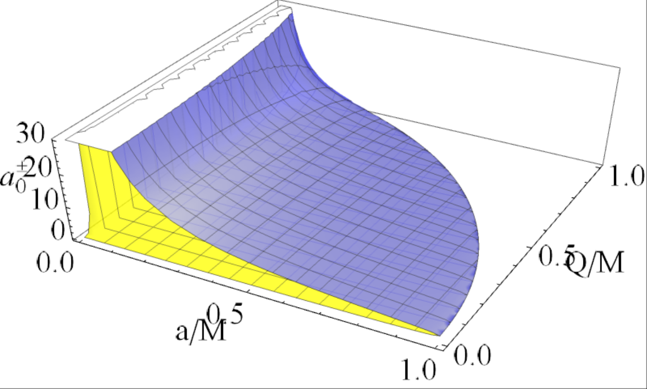

We can see that in the extended plane it is necessary to consider the entire range of parameter values , including the BH case to describe the NSs. For the equatorial plane, the analysis carried out for the case is confirmed also in presence of an electric charge. For predominant spins, any curve constant crosses the horizons at some points. We also see the bending of the curves limited above from the inner horizon , confirming the results of Sec. IV, although with differences which are evident as the electric charge increases.


The generalization of the analysis of Fig. (10) is presented in Figs. (27) and (28). We will not enter into the details of this analysis; instead, we only mention that in the KN case a more articulated situation for the Killing throat and bottleneck appears, when the effects of the electric charge are combined with those of the frame-dragging. The frequencies are plotted as functions of for different values of the charge and spin in Fig. (26). In these plots, the static and axisymmetric cases are compared and the contribution of an electric charge are confronted with those of weak NS geometries. In the static geometries, the Killing throat and bottleneck still appear, while the effects of the rotation emerge as a disruption of the symmetry around the axis of the static case and become evident in the coalescence phases of the horizons.


 |


 |
Figures (29), (31) and (30), on the other hand, show the solutions of and defining the Killing bottlenecks of naked singularities, which are generalizations of the analysis presented in Fig. (5) for the case (Kerr spacetime). The surfaces are shown in Fig. (30), giving a view of the solutions for the light surfaces in the off-equatorial case.


 |


 |

 |


VI Concluding remarks and future perspectives
In this work, specially in Sec. III, we explored the Killing throats and bottlenecks, arising from the properties of stationary observers in the Kerr geometries. In the case of WNSs (), the Killing throats show “restrictions”, which we identify as Killing bottlenecks. To explore the properties of the bottlenecks, we introduced in Sec. (IV) the concept of extended plane, which is a graph relating a particular characteristic of a spacetime in terms of the parameters entering the corresponding spacetime metrics. More precisely, the analysis of some peculiar characteristics of the bottlenecks, defined as horizons remnants, indicated some links between BHs and NSs (and in particular WNSs). To compare the BH and NS characteristics, it was convenient to introduce in Sec. IV the concept of metric bundles, i.e., curves in the extended plane , representing a collection of metrics defined by a particular photon orbital frequency, named metric bundle frequency. The bundle frequencies (and the orbital limiting frequencies in any point on the equatorial plane of any spacetime of the family) are all and only the frequencies of the horizon defined in the extended plane. This analysis has been done mainly on the equatorial plane of axisymmetric geometries. Metric bundles show, in fact, the remarkable property to be tangent to the horizon curve in the extended plane, the space where the curves representing the metric bundles are defined. In the case of the the equatorial plane of the Kerr metric, the extended plane is essentially equivalent to the function that relates the frequency with the spin. Notably, the metric bundle associated to the extreme Kerr BH corresponds to a regular curve tangent to the horizon with bundle origin . As proved in Sec. IV, all the metric bundles are tangent to the horizon in the extended plane and the horizon emerges as the envelope surface of the metric bundles in . A bundle frequency corresponds to one limiting photon orbital frequency for all BHs or some BHs and NSs geometries. The bundle frequency coincides with the frequency at the (inner or outer) horizon curve, which is tangent to the metric bundle. On the other hand, the metric bundles are all defined by all and only the frequency of the horizon in . Viceversa, all the horizon frequencies in the extended plane are metric bundle frequencies. In Sec. V, we consider the static and electrically charged Reissner-Nordström spacetime and the Kerr-Newman axisymmetric electrovacuum solution and show that the bending (closing) of the curves of the metric bundles is due to the rotation of the gravitational source. Therefore, we can say that the horizons frequencies determine the BHs and NSs limiting photon orbital frequencies. This fact establishes a connection between BHs and NSs: the inner BH horizon is connected to BH and WNS origin bundles, whereas the outer horizon sets the BHs-SNSs correspondence. In the extended plane, NSs are associated with portions of the horizon. In this sense, the inner horizon is partially constructed by BH metric bundles. The inner horizon is associated with WNS origins. This last property turns out to be related to the Killing bottlenecks appearing in the light surfaces. Interestingly, the outer horizon in is generated by SNSs metric bundles only. This fact has the interesting consequence that only the horizon frequencies determine the frequencies at each point, , on the equatorial plane of a Kerr BH or NS geometry: all the frequencies on the equatorial plane are only those of the horizon in , the horizon in contains information about all limiting photon orbits also in NS spacetimes. In Secs. III and IV, we have also introduced the concept of inner horizon confinement. In this sense, NSs are “necessary” for the construction of horizons. The outer horizon is associated with a NS (the bundle origin) in the extended plane and the inner horizon to a WNS or a BH. Therefore, we believe that this result could be of interest for the investigation of gravitational collapses in which connections between NS and BH solutions are expected and emerge Goswami:2006ph; CS181; Manko:2018yrc.
Some further aspects of these properties are currently under investigation. Firstly, it would be necessary to further analyze the off-equatorial case and test the results of Sec. IV in other kinds of geometries. In a future analysis, we shall analyze other axisymmetric spacetimes admitting Killing horizons and consider the possible thermodynamic implications of the results discussed here, particularly, in relation to the possibility of formulating the BH thermodynamic laws in terms of metric bundles. We also point out that metric bundles and horizons remnants seem to be related to the concept of pre-horizon regimes. There is a pre-horizon regime in the spacetime when there are mechanical effects allowing circular orbit observers, which can recognize the close presence of an event horizon. This concept was introduced in de-Felice1-frirdtforstati and detailed for the Kerr geometry in de-FeliceKerr; de-Felice-anceKerr. The pre-horizon was identified and analyzed in de-Felice-first-Kerr, leading to the conclusion that a gyroscope would observe a memory of the static case in Kerr metric. Clearly, this aspect could be of relevance during the gravitational collapse de-Felice3; de-Felice-mass; de-Felice4-overspinning; Chakraborty:2016mhx.
We now summarize the main aspects of our analysis focusing on the possible interpretation of the main results.
(i) We identified bottlenecks essentially as horizon remnants. Similar interpretations have been presented in de-Felice1-frirdtforstati; de-FeliceKerr; de-Felice-anceKerr; de-Felice-first-Kerr, by using the concept of pre-horizons, and in Tanatarov:2016mcs, by analyzing the so-called whale diagrams. These structures could play an important role for describing the formation of black holes and for testing the possible existence of naked singularities. Notably, the concept of remnants, as expressed here, refers to and evokes a sort of spacetime “plasticity”, which naturally led to the introduction in Sec. (IV) of the concept of the extended plane. In this new frame, we found several properties emerging from and affecting the spacetime geometries when we consider an entire family of solutions as a unique geometric object.
(ii) Considering the Kerr family as a single object, the geometric quantities (for example, the horizons) defined for a single solution acquire a completely different significance when considered for the entire family.
(iii) Considering metric bundles with WNS, we found that the inner horizon is confined in the metric bundle framework.
(iv) We proved the existence of a connection between black holes and naked singularities. To each BH corresponds the pair (WNS, SNS) or the pair (BH, SNS). This correspondence is important for the definition of the Killing horizons.
(v) We proved that WNSs (SNSs) are necessary for the construction of the inner (outer) Killing horizon. This result could shed light on the physical meaning of NSs solutions.
To conclude, we present a schematic summary of the main results presented in this work.
- •
Analysis of Killing throats and definition Killing bottlenecks for particular naked singularities–Section III. To define Killing throats, we study the limiting photons surfaces and frequencies which are defined in Eq. (11) and Eq. (8), respectively. We also interpret bottlenecks as horizons remnants in weak naked singularities.
- •
Inner horizon confinement–Sec. III. In Eq. (13), we identify the photon orbits characterized by the horizons orbital frequencies. The radii represent the set of photon orbits with frequencies at the BH horizons—Eq. (13)–Fig. 1. The inner horizon confinement, according to the constraints on , is in agreement with the confinement of the metric bundles containing BHs and WNSs (see Sec. IV).
- •
Definition of the extended plane and metric bundles in Sec. IV. Metric bundles are curves in tangent to the horizons characterized by the limiting photon frequency or .
- •
Tangency condition and horizon construction in the extended plane. We demonstrate that the horizon curve corresponds to the envelope surface of the metric bundles. All the metric bundles are tangent to the horizon curve and all the points of the horizons are associated to one and only one metric bundle tangent to that point– Figs. 14, 15, 16 and Tables 3 and 2. Consequently, all the limiting photon orbital frequencies (on the equatorial plane) are all and only the frequencies of the horizon curve in , related to two metric bundles, with frequencies and , respectively. Particularly, through the relationship between metric bundles and horizons in , a NS or BH metric can be parameterized in terms of the horizon frequency identified by the corresponding metric bundle. The inner and outer horizons in correspond to envelope surfaces. We analyze the lines constant (i.e. a single spacetime of the metric bundle) and constant in the extended plane–Fig. 8 and classify the singularities according to the horizon construction as shown in Fig. (13), i.e., strong naked singularities, , having with for and for ; WNS–weak naked singularities with and with for , and for .
- •
Demonstration of the confinement of metric bundles with origin in BHs and WNSs and identification and study of the corresponding bundles. In Table 2, we proved the confinement of the bundles in the extended plane delimited by the inner horizon curve. The horizon and bundle frequencies are related by the relation .
- •
Properties of horizons and bundles. For the entire family of Kerr geometries, we established the relations between metric bundles and horizons. We found two relations which can be specified in detail as follows. Relations I: , , where (, )–Fig. (13). Relation II: , , (or equivalently ), where and –Fig. 14.
- •
Properties of specific spacetimes. We studied the metric bundles corresponding to a single BH spacetime (with equal tangent spin ). We analyzed the Kerr spacetime in terms of metric bundles–Sec. IV.
- •
Proof of the BH-NS relation through the properties of the corresponding metric bundles.
- •
Analysis of the frequencies of the spacetime by using the maximum crossing of two metric bundles–Eq. (22). We proved he existence of the corresponding metric bundles and analyzed its significance for the horizon construction and properties of a BH spacetime–Tables 2 and 3; Figs. 13,14,15,15,16,17 and Eqs. (19) and (27).
- •
Identification of the Killing throats and bottlenecks and metric bundles in the static and charged Reissner Nordström solution and in the axisymmetric, electrically charged, Kerr-Newmann spacetime. We proved that the bending (curvature) of the Kerr metric bundles in is related to the frame-dragging of the spinning spacetimes. We noticed the different roles played by the electric and rotational charges –Eq. (28). We studied the metric bundles in terms of the electric charge –Eq. (35). In Sec. A, we analyzed the off-equatorial case of the Kerr and Kerr-Newman geometries. In Sec. B, we considered the relations between the areas of the horizon and of the metric bundles regions in the extended plane.
Acknowledgements.
D.P. acknowledges partial support from the Junior GACR grant of the Czech Science Foundation No:16-03564Y. D.P. is grateful to Donato Bini, Fernando de Felice and Andrea Geralico for discussing many aspects of this work. This work was partially supported by UNAM-DGAPA-PAPIIT, Grant No. 111617, and by the Ministry of Education and Science of RK, Grant No. BR05236322 and AP05133630.Appendix A Analysis of the Kerr and Kerr-Newman geometries: the off-equatorial case
In this appendix, we summarize the analysis presented in Secs. III, IV and V for off-equatorial stationary observers in Kerr and Kerr-Newman spacetimes. We focus on the presentation of the corresponding plots which contain all the relevant information for this case.


 |


 |


 |


 |


 |


 |

 |
Appendix B Areas of the horizon and of the metric bundles regions in
In this section, we analyze the area of the regions of in Fig. 8 bounded by the curves for constant, between and , including the entire collection of spacetimes bounded by . We compare this region with the (inaccessible) section in bounded by the horizons .
First, note that each region bounded by can be decomposed into other non-disjoint metric bundles. In fact, as can be seen in Fig. 8, the metric bundles cross each other in . This corresponds to the fact that for a fixed point , different frequencies are possible, i.e., a light-like particle can have different orbital frequencies corresponding to the two solutions . To explore this aspect and also the BH-NS connection, we introduce the radii
| (41) |
which are plotted in Fig. 11 as functions of the frequency . It is clear that the functions are limiting radii. A generalization of this study is also discussed in Sec. V, where we consider the Reissner-Nordström and Kerr-Newman geometries.
The areas correspond to the regions of the extended plane bounded by and are confronted here with the areas of the region bounded by the horizons . An analysis of these areas is shown in Figs. 32. We can write the areas as functions of the frequency of the metric bundles or, equivalently, the spin origins , as follows
| (42) | |||
| (43) | |||
where dimensionless quantities have been used. We also define the quantities and , where is a function of the frequency of the metric bundle and of the radius . Moreover, is an integration constant. From Fig. 32, it is clear that the area is a decreasing function of the frequency , which is in agreement with the results of Fig. 8. Indeed, the metric bundles shrink at the origins , that is, for frequencies , where are all contained in . Viceversa, the area grows as the spin-mass ratio of the NS increases. The right panel of Fig. 32 shows an area constant with respect to the frequency and the radius . Special cases correspond to the limiting geometries and .


Finally, the evaluation of the areas in takes into account the curvature of the curves in the plane. Therefore, it is necessary to consider some relative quantities reported below and represented in Fig. (32). Considering the quantities
| (44) |
and using in Eq. (16), we can obtain the area of the regions bounded by the curves , between the points and . The curves bending the area are related to solutions of the equation , which is solved for , while the only solutions are for the frequencies in the frequency range , where the distance between the two curves is extreme. These quantities, considering the variation of with respect to the frequencies and the radius respectively, are related to the curvature of the , where the extreme radius as function of the frequency is
| (45) | |||
| (46) |
References
- (1) F. de Felice, Mont. Notice R. astr. Soc. 252, 197-202, (1991).
- (2) F. de Felice and S. Usseglio-Tomasset, Class. Quantum Grav. 8., 1871-1880 (1991).
- (3) P. T. Chrusciel, J. Lopes Costa and M. Heusler, Living Rev. Rel. 15, 7 (2012).
- (4) R. M. Wald, Class. Quant. Grav. 16, A177 (1999).
- (5) R. M. Wald, Living Rev. Relativ. 4(1), 6 (2001).
- (6) Z. Li and C. Bambi, Phys. Rev. D 87, 124022 (2013).
- (7) T. Jacobson and T. P. Sotiriou, J. Phys. Conf. Ser. 222, 012041 (2010).
- (8) S. L. Shapiro and S. A. Teukolsky, Phys. Rev. Lett. 66, 994 (1991).
- (9) R. Goswami, P. S. Joshi and P. Singh, Phys. Rev. Lett. 96, 031302 (2006).
- (10) J. P. S. Lemos, G. M. Quinta and O. B. Zaslavskii, Phys. Rev. D 93, no. 8, 084008 (2016)
- (11) D. Pugliese, H. Quevedo and R. Ruffini, in Proceedings, 12th Marcel Grossmann Meeting on General Relativity, Paris, France, July 12-18, 2009. Vol. 1-3,” p.1017-1021, edited: T. Damour, R. T. Jantzen and R. Ruffini, Singapore, Singapore: World Scientific (2012).
- (12) D. Pugliese, H. Quevedo and R. Ruffini, Phys. Rev. D 84, 044030 (2011).
- (13) D. Pugliese, H. Quevedo and R. Ruffini, Phys. Rev. D 83, 024021 (2011).
- (14) D. Pugliese, H. Quevedo and R. Ruffini, Phys. Rev. D 83, 104052 (2011).
- (15) D. Pugliese, H. Quevedo and R. Ruffini, Phys. Rev. D 88, 024042 (2013).
- (16) D. Pugliese and H. Quevedo, Eur. Phys. J. C 75, 5, 234 (2015).
- (17) D. Pugliese, H. Quevedo and R. Ruffini, Eur. Phys. J. C 77, 4, 206 (2017).
- (18) D. Pugliese and H. Quevedo, Eur. Phys. J. C 78, 1, 69, (2018).
- (19) C.J.S. Clarke, F. De Felice, Gen. Rel. Grav., 16, 2, 139-148 (1984).
- (20) D. Bini, F. de Felice, Gen. Rel. Grav., 47, 131, 11, (2015).
- (21) F. de Felice, A&A, 34, 15 (1974).
- (22) F. de Felice , Nature 273, 429–431 (1978).
- (23) C. Chakraborty, M. Patil, P. Kocherlakota, et al., Phys. Rev. D 95, 8, 084024 (2017).
- (24) M. Blaschke, Z. Stuchlík, Phys. Rev. D 94 , 8, 086006 (2016).
- (25) M. Bejger, T. Piran, M. Abramowicz and F. Hakanson, Phys. Rev. Lett. 109, 121101 (2012).
- (26) Z. Stuchlik, P. Slany, G. Torok and M. A. Abramowicz, Phys. Rev. D 71, 024037 (2005).
- (27) Z. Stuchlik and J. Schee, Class. Quant. Grav. 29, 065002 (2012).
- (28) K. i. Nakao, P. S. Joshi, J. Q. Guo, et al. Phys. Lett. B 780, 410 (2018).
- (29) S. Gao and Y. Zhang, Phys. Rev. D 87, 4 044028 (2013).
- (30) Z. Stuchlik, Bull. Astron. Inst. Czech. 32, 68 (1981).
- (31) P. Pradhan and P. Majumdar, Eur. Phys. J. C 73, 6 2470 (2013).
- (32) M. Kolos and Z. Stuchlík, Phys. Rev. D 88 065004, (2013).
- (33) Z. Stuchlik and J. Schee, Class. Quant. Grav. 27, 215017 (2010).
- (34) I. V. Tanatarov and O. B. Zaslavskii, Gen. Rel. Grav. 49, no.9, 119 (2017).
- (35) S. Mukherjee and R. K. Nayak, Astrophys. Space Sci. 363 no.8, 163 (2018).
- (36) O. B. Zaslavskii, Phys. Rev. D 98, no.10, 104030 (2018).
- (37) E. Barausse, V. Cardoso, and G. Khanna, Phys. Rev. Lett. 105, 261102 (2010).
- (38) P. S. Joshi, Gravitational Collapse and Spacetime Singularities, Cambridge Monographs on Mathematical Physics, New York (2007).
- (39) B. Giacomazzo, L. Rezzolla and N. Stergioulas, Phys. Rev. D 84, 024022 (2011).
- (40) A. Helou, I. Musco and J. C. Miller, Class. Quant. Grav. 34, 13, 135012 (2017).
- (41) R. M. Wald and V. Iyer, Phys. Rev. D 44, 3719 (1991).
- (42) J. Gariel, N. O. Santos and J. Silk, Phys. Rev. D 90, 063505 (2014).
- (43) N. Pelavas, N. Neary and K. Lake, Class. Quant. Grav. 18, 1319 (2001).
- (44) C. Herdeiro and E. Radu, Phys. Rev. D 89, 1240 18 (2014).
- (45) V. Cardoso, P. Pani, M. Cadoni and M. Cavaglia, Phys. Rev. D 77, 124 044 (2008).
- (46) N. Comins and B. F. Schutz, Proc. R. Soc. A 364, 1717 211-226 (1978).
- (47) A. V. Frolov and V. P. Frolov, Phys. Rev. D 90, 12, 124010, (2014).
- (48) Z. Stuchlik, Bull. Astron. Inst. Czech 31, 129 (1980).
- (49) Z. Stuchlik, J. Schee, Class. Quant. Grav. 30, 7, 075012 (2013).
- (50) J. Schee and Z. Stuchlik, JCAP 1304, 005 (2013).
- (51) G. Torok and Z. Stuchlik, Astron. Astrophys. 437, 775 (2005).
- (52) J. Biéak, Z. Stuchlik, and V. Balek, Bull. Astron. Inst. Czech 40, 2 65–92 (1989).
- (53) M. Patil and P. S. Joshi, Class. Quant. Grav. 28, 235012 (2011).
- (54) O. B. Zaslavskii, Gen. Rel. Grav. 48, 10, 132 (2016).
- (55) R. Goswami and P. S. Joshi, Phys. Rev. D 76 084026 (2007).
- (56) T. Crisford and J. E. Santos Phys. Rev. Lett. 118, 181101 (2017).
- (57) V. S. Manko and E. Ruiz, arXiv:1803.03301 [gr-qc] (2018).
- (58) F. de Felice, Class. Quantum Grav. 11, 1283-1292 (1994).
- (59) F. de Felice and S. Usseglio-Tomasset, Gen. Rel. Grav. 28, 2 (1996).
- (60) F. de Felice and S. Usseglio-Tomasset, Gen. Rel. Grav. 24, 10 (1992).
- (61) F. de Felice and L. Di G. Sigalotti Ap.J. 389, 386-391 (1992).
- (62) F. de Felice and Y. Yunqiang, Class. Quantm Grav. 10, 353-364 (1993).