Circulation in high Reynolds number isotropic turbulence is a bifractal

Figure 1 shows circulation traces for inertial range separations, normalized by its standard deviation, along the length of the simulation domain of size $L_{0}$, at the Taylor scale Reynolds number, $R_{\lambda}=1300$. Two different inertial separations $r$ corresponding to the lower end and the middle of the inertial range plateau in $-\langle(\Delta_{r}u)^{3}\rangle/r\langle{\epsilon}\rangle$, are shown here. These particular signals do not show frequent excursions to very high values (unlike highly intermittent phenomena).

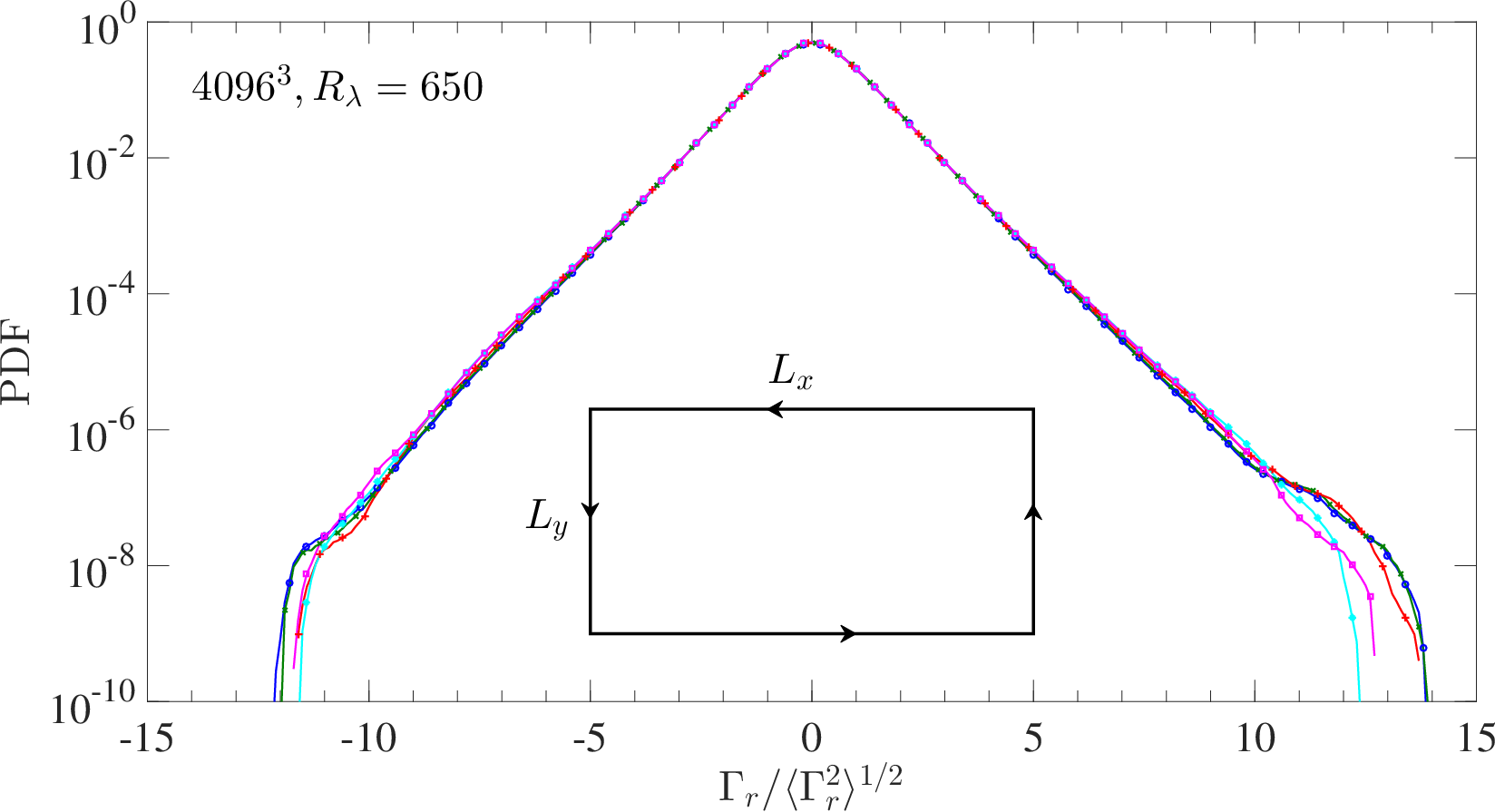
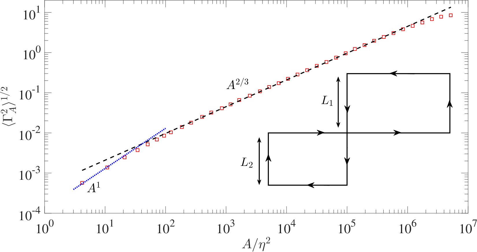
Figure 2 shows the PDFs of $\Gamma_{r}$ for a number of rectangular loops of the same area but differing aspect ratios. The data collapse to a very good accuracy. Even though the result will have to be confirmed for loops of different shapes, this figure supports the expectation that only the area of the loop, not its shape, decides the PDF of circulation. It is thus sometimes convenient to use the symbol $\Gamma_{A}$ to describe the circulation around a loop of area $A$; henceforth, when we speak of $\Gamma_{r}$, it means circulation around a square of side $r$.

The inset to 3 shows a figure-$8$ loop with two different squares touching at a common vertex. If K41 is valid, it readily follows that the standard deviation of circulation $\langle\Gamma_{A}^{2}\rangle^{1/2}\sim(L_{1}^{2}+L_{2}^{2})^{2/3}=A^{2/3}$. On the other hand, if one traverses along the loop in the direction of the arrows marked on the loop, the areas circumscribed by the two squares will have different signs. If the resulting vector area is the right quantity to use, the standard deviation $\langle\Gamma_{A}^{2}\rangle^{1/2}$ for the figure-$8$ loop should scale as

$$\langle\Gamma_{A}^{2}\rangle^{1/2}\sim(L_{1}^{2}-L_{2}^{2})^{2/3}=(\Delta(L_{1}+L_{2}))^{2/3}\sim A^{1/3}\;,$$

(3)

since, $\Delta=L_{1}-L_{2}$ is a fixed constant. The main part of Fig. 3 shows convincingly that the mean-square circulation varies as $A^{2/3}$, where $A$ is the scalar sum of the areas of the two loops, for most of the range. For small $A$, the variance is clearly linear in $A$ as expected from Taylor expansion, whereas it saturates for large $A$ because of many cancellations.

As already stated, straightforward application of K41 shows that $\Gamma_{r}\sim r^{4/3}$. Migdal Migdal 1994 argued that the PDF of $\Gamma_{r}$ decays as some power of ${\Gamma_{r}}^{3}/r^{4}$. We show the PDF of ${\Gamma_{r}^{3}}/{r^{4}}\langle{\epsilon}\rangle$ in Fig. 4 for various inertial range separations. The PDFs show good collapse, with some deviations in the negative PDF tails; the two insets, highlighting the positive and negative tails of the PDF, are not power laws. They can be fitted nominally by unequal stretched exponentials, as described in the caption to Fig. 4. The mean and the mean square of this distribution yield the third-order and sixth-order moments of circulation. These and other moments are computed separately in Sec. III.1.

The results so far are already interesting and tantalizing because they contain the suggestion that K41 may have currency for circulation. This would be quite unlike, say, for velocity increments or enstrophy density. We now explore this feature further by computing the scaling properties.

We first evaluate various even order moments of $\Gamma_{r}$ and show moments $\langle\Gamma_{r}^{p}\rangle$ for $p=2,4,6$ and $8$ for $R_{\lambda}=1300$ as functions of $r$ in Fig. 5. They all display proper power laws, $\langle\Gamma_{r}^{p}\rangle\sim r^{\lambda_{p}}$, in the inertial range, as reinforced by the constancy of the local slopes, shown in the inset of Fig. 5.

The odd moments of $\Gamma_{r}$ do not display equally clean power laws because they have negligible intensity via cancellation, which leads to poor convergence. Their scaling improves if one considers absolute values of circulation, $\langle|\Gamma_{r}|^{p}\rangle\sim r^{\lambda_{|p|}}$ (while, obviously, those of even orders remain unchanged). Absolute values enable us to define scaling exponents for fractional $p$ as well, up to (but not including) $p=-1$, for which the moments diverge Chen et al. 2005. The practice of using absolute moments for odd orders is justified, at least a posteriori, as long as the exponents so obtained are monotonic when plotted together with even-order data. This monotonic behavior is not quite true for velocity structure functions even for very high Reynolds numbers typical of atmospheric flows (see Ref. Sreenivasan and Dhruva 1998 at $R_{\lambda}=10,340$) but seems to hold for circulation for which the absolute moment data do not zigzag with respect to even-order data.

In Fig. 6 we plot the scaling exponents ${\lambda_{|p|}}$ for circulation as a function of the power index $p$ for all orders at $R_{\lambda}=1300$. The exponents seem to organize themselves into two straight lines, one below about 3 and the other above it. The low-order data can be fitted asymptotically by the K41 line, ${\lambda_{|p|}}=4p/3$, but one needs a different line with a smaller slope for higher orders. The latter line (with the slope of 7/6 and an intercept of 1/2) can be expressed in terms of the $\beta$-model Frisch et al. 1978,

$${\lambda_{|p|}}=\frac{4p}{3}+(3-D)(1-\frac{p}{3})\;,$$

(4)

with $D\approx 2.5$ as the self-similarity dimension Mandelbrot 1974; Frisch et al. 1978.

We have so far considered results for the two highest Reynolds numbers of the dataset computed by us. It is instructive to examine how the results depend on the Reynolds number, and assess the asymptotic state.

We have already seen the PDFs in two forms: The PDF for circulation around various shapes of loops within the inertial range in Fig. 2 and those for ${\Gamma_{r}^{3}/r^{4}\langle{\epsilon}\rangle}$ in Fig. 4. We now plot the PDFs of $\Gamma_{r}$ for several values of $r$ in the inertial range, normalized by their own standard deviations. The PDFs collapse on each other for magnitudes below about 5 standard deviations (see inset (a)) and differ mostly in the tails. This shows that we do not have perfect self-similarity. The PDFs also depart strongly from the Gaussian distribution indicated by the dashed line, both at the tails and the core region (see inset (a)). The peaks of the PDFs gradually drop towards the Gaussian value of about 0.4 through the inertial range, as can be seen more explicitly in inset (b), but the tails are of the stretched exponential type $\sim exp(-\beta\Gamma_{r}^{{\alpha(r)}})$. The stretching exponent $\alpha(r)$ is plotted in inset (c) of Fig. 7 as a function of the inertial range separation $r$; we have $\alpha(r)$ varying weakly with $r$, supporting the notion that circulation has weak intermittency Vainshtein et al. 1994. We note that the variation of $\alpha(r)$ in the inertial range is gentler than that of the corresponding stretching exponents of velocity increments, which are known to rapidly change with scale Kailasnath et al. 1992.

The circulation flatness is defined as

$$F(r)\equiv\frac{\langle\Gamma_{r}^{4}\rangle}{\langle\Gamma_{r}^{2}\rangle^{2}}\;.$$

(5)

Figure 8 shows that $F(r)$ varies through the inertial range $(\eta\ll r\ll L)$ but its evolution with Reynolds number is the more interesting point; the figure also compares $F(r)$ at three different Reynolds numbers. At $R_{\lambda}=240$, $F(r)$ increases smoothly from the Gaussian value of $3$, for $r\sim O(L)$, to the dissipation range limit of $\langle\omega^{4}\rangle/\langle\omega^{2}\rangle^{2}$, where $\omega$ is the vorticity component normal to the plane of circulation. With increasing $R_{\lambda}$, however, $F(r)$ appears to develop a plateau in the inertial range, indicating that it may be approaching a constant, independent of scale. The inset of Fig. 8 compares the circulation flatness to those of the longitudinal and transverse velocity increments at $R_{\lambda}=1300$. Here, the transverse increment $\Delta_{r}v\equiv v(x+r)-v(x)$, where the separation distance $r$ is transverse to the velocity component $v$. Even at $R_{\lambda}=1300$, the flatness factors of both $\Delta_{r}u$ and $\Delta_{r}v$ smoothly grow with decreasing scale, showing that the velocity increments are highly intermittent, whereas $F(r)$ displays the tendency towards constancy, suggesting that $\Gamma_{r}$ at high Reynolds numbers is only weakly intermittent. It should be stressed that, at lower $R_{\lambda}$, all flatness factors of $\Gamma_{r}$, $\Delta_{r}u$ and $\Delta_{r}v$ increase rapidly with decreasing scale in the inertial range, as already shown in Refs. Cao et al. 1996; Zhou et al. 2008.

Our point is that the flatness $F(r)$ has the potential to become a constant in the inertial range of $r$ as the Reynolds number increases further. If so, this will be the intermittency-free limit in which we expect the logarithmic local slope of flatness $d[\log F(r)]/d[\log r]\to 0$ in the inertial range. To quantify this approach to the intermittency free limit, we plot the logarithmic local slope of $F(r)$ as a function of spatial separation in the inset of Fig. 9 for two different Reynolds numbers. For $R_{\lambda}=1300$, the local slopes are closer to zero over a wider range of inertial scales than for $R_{\lambda}=240$. The peaks of the flatness local slopes decrease linearly with $R_{\lambda}$ as shown in Fig. 9, suggesting that it will be zero at $R_{\lambda}\approx 1900$. This result should be regarded merely as an indication and will be discussed further in Sec. IV.1 below.

Figure 10 shows the behavior of $\delta_{\lambda_{p}}$, the difference between the measured scaling exponents and the corresponding Kolmogorov values, for moment orders $4$, $6$, $8$ and $10$, as functions of the Reynolds number. For each order, this difference seems to approach K41 roughly as a power law. The rates of approach vary inversely with the order of the moment. We cannot speculate about the behaviors at infinitely large Reynolds numbers, but may expect that this behavior will persist up to some higher Reynolds number. The fact that the approach to the K41 values is slower for the high-order moments suggests that, in principle, the scaling will remain a bifractal for all finite Reynolds numbers, with the “phase transition” point moving to a higher $p$ with increasing Reynolds numbers. In practice, however, moments may fall on the K41 line for sufficiently high values of $p$ that the bifractal behavior may essentially yield place to a space-filling monofractal.

Since circulation is very closely related to vorticity, it is natural to ask why the simplicity that is apparent in circulation does not translate to locally averaged enstrophy density, which is known to be a strongly multifractal quantity Meneveau et al. 1990; Yeung et al. 2018. The corresponding question is relevant also with respect to velocity increments. We address this issue here briefly.

The area integral formula for circulation from Eq. 1 reads as

$$\Gamma_{r}=\int\omega dA\;,$$

(6)

where $\omega$ is the vorticity component perpendicular to the loop with area, $A=r^{2}$, along an arbitrary direction. Taking the square of above equation and invoking Schwarz’s inequality, we get

	$\displaystyle\Gamma_{r}^{2}$	$\displaystyle=$	$\displaystyle\Big[\int\omega dA\Big]^{2}\;,$		(7)
		$\displaystyle\leq$	$\displaystyle r^{2}\int\omega^{2}dA\;.$		(8)

Taking averages on both sides of the above inequality we get

$$\langle\Gamma_{r}^{2}\rangle\leq r^{2}\Big\langle\int\omega^{2}dA\Big\rangle\;.$$

(9)

Now, define $\Omega=\omega_{i}\omega_{i}$ and use statistical isotropy. Then, for any general power, $p\geq 1$,

$$\Big\langle\Big(\int\omega^{2}dA\Big)^{p}\Big\rangle\leq\frac{1}{3}\Big\langle\Big(\int\Omega dA\Big)^{p}\Big\rangle,\$$

(10)

with equality valid for $p=1$. Substituting Eq. 10 in Eq. 9 for $p=1$, we obtain

$$\langle\Gamma_{r}^{2}\rangle\leq\frac{1}{3}r^{2}\Big\langle\int\Omega dA\Big\rangle\;\;.$$

(11)

We can define the local 2D average of enstrophy as

$$\Omega_{r}\equiv\frac{1}{r^{2}}\int\Omega dA\;,$$

(12)

and rewrite Eq. 11 as

$$\langle\Gamma_{r}^{2}\rangle\leq\frac{1}{3}r^{4}\langle\Omega_{r}\rangle\;.\\$$

(13)

Generalizing the above inequality to any even power $2p$, we get

$$\langle\Gamma_{r}^{2p}\rangle\leq\frac{1}{3}{r}^{4p}\langle\Omega_{r}^{p}\rangle\;.\\$$

(14)

This inequality shows that the moments of locally averaged enstrophy are quite likely to be larger than those of circulation, and it is this that states that the multifractal character of enstrophy density need not necessarily carry over to circulation.

With respect to moments of the velocity increments, we can use the second hypothesis of Kolmogorov (Kolmogorov 1962) which can be expressed as

$$\Delta_{r}u=V(r\epsilon_{r})^{1/3}\equiv V^{\prime}(r\nu\Omega_{r})^{1/3},$$

(15)

where $V$ and $V^{\prime}$ are universal variables with the constraint that, $\langle V^{3}\rangle=\langle V^{\prime 3}\rangle=-4/5$, and $\nu$ (as before) is the kinematic viscosity. Then, Eq. 14 becomes

$$\langle\Gamma_{r}^{2p}\rangle\leq\frac{1}{3}{r}^{3p}\frac{\langle(\Delta_{r}u)^{3p}\rangle}{\nu^{p}\langle V^{\prime 3p}\rangle}\;.\\$$

(16)

Under homogeneity, the first moments of dissipation, enstrophy and their local averages are related as $\nu\langle\Omega_{r}\rangle=\langle\epsilon_{r}\rangle=\langle\epsilon\rangle$, using which, inequality (14) (corresponding to $p=1$) can be written as

$$\psi(r)\equiv\frac{\langle\Gamma_{r}^{2}\rangle\nu}{r^{4}\langle\epsilon\rangle}\leq\frac{1}{3}\;.\\$$

(17)

Using $p=1$ and the inertial range result $\langle(\Delta_{r}u)^{3}\rangle=(-4/5)r\langle\epsilon\rangle$, we end up with the same inequality as Eq. 17. Inequality 17 is more general, since it shows that $\psi(r)$ is bounded for all $r$.

As a check, we note that in the dissipative limit $r\to 0$, we have

$$\lim_{r\to 0}\psi(r)=\lim_{r\to 0}\frac{\langle\Gamma_{r}^{2}\rangle\nu}{r^{4}\langle\epsilon\rangle}=\frac{\langle\omega^{2}\rangle\nu}{\langle\epsilon\rangle}=\frac{1}{3}\frac{\langle\Omega\rangle\nu}{\langle\epsilon\rangle}=\frac{1}{3}\;,$$

(18)

where the relation $\langle\Omega\rangle=3\langle\omega^{2}\rangle$ uses isotropy.

It is interesting to consider the double limit of $\psi(r)$, namely

$$\lim_{\nu\to 0}\lim_{r\to 0}\frac{\langle\Gamma_{r}^{2}\rangle}{r^{4}}\left[\frac{\nu}{\langle\epsilon\rangle}\right]\;.$$

(19)

Since the mean dissipation is known not to depend on viscosity Sreenivasan 1984; Sreenivasan 1998; Pearson et al. 2002; Kaneda et al. 2003, the term within square brackets that is $r$-independent, tends to $0$ in the asymptotic limit. This means that in the small-$r$ limit we have, $\langle\Gamma_{r}^{2}\rangle/r^{4}=\langle\omega^{2}\rangle\to\infty$ for high Reynolds numbers. It follows that vorticity can attain very high moment values in turbulent flows even when those of circulation are bounded. This observation does not necessarily imply that circulation (around finite contours) is always bounded, but it does suggest that it is a more tractable quantity to work with, as compared to vorticity.

Figure 11 shows that the DNS data are quite consistent with the dissipative limit. Furthermore, $\psi(r)$ at different Reynolds numbers shows good collapse for $r\ll L$, where $L$ is the integral scale.

These arguments show that the simplicity in the structure of circulation does not contradict the known multifractal properties of velocity increments or enstrophy density. We thus believe that we have covered new ground here.

References

- da Vinci (2010) L. da Vinci, The notebooks of Leonardo da Vinci, edited by J. P. Richter (Pac PS, 2010).
- Kaneda et al. (2003) Y. Kaneda, T. Ishihara, M. Yokokawa, K. Itakura, and A. Uno, Phys. Fluids 15, L21 (2003).
- Kolmogorov (941a) A. N. Kolmogorov, Dokl. Akad. Nauk. SSSR 30, 299 (1941a).
- Monin and Yaglom (1975) A. S. Monin and A. M. Yaglom, Statistical Fluid Mechanics, Vol. 2 (MIT Press, 1975).
- Benzi et al. (1984) R. Benzi, G. Paladin, G. Parisi, and A. Vulpiani, J. Phys. A: Math. Gen. 17, 3521 (1984).
- Frisch (1995) U. Frisch, Turbulence (Cambridge University Press, 1995).
- Eyink (1995) G. L. Eyink, J. Stat. Phys. 78, 353 (1995).
- Sreenivasan and Antonia (1997) K. R. Sreenivasan and R. A. Antonia, Annu. Rev. Fluid Mech. 29, 435 (1997).
- Migdal (1994) A. A. Migdal, Int. J. Mod. Phys. A 9, 1197 (1994).
- Umeki (1993) M. Umeki, J. Phys. Soc. Jpn. 69, 3788 (1993).
- Sreenivasan et al. (1995) K. R. Sreenivasan, A. Juneja, and A. K. Suri, Phys. Rev. Lett. 75, 433 (1995).
- Cao et al. (1996) N. Cao, S. Chen, and K. R. Sreenivasan, Phys. Rev. Lett. 76, 616 (1996).
- Benzi et al. (1997) R. Benzi, L. Biferale, M. V. Struglia, and R. Tripiccione, Phys. Rev. E 55, 3739 (1997).
- Zhou et al. (2008) Q. Zhou, C. Sun, and K. Q. Xia, J. Fluid Mech. 598, 361–372 (2008).
- Yeung et al. (2015) P. K. Yeung, X. M. Zhai, and K. R. Sreenivasan, Proc. Nat. Acad. Sci. 112, 12633 (2015).
- Yeung et al. (2018) P. K. Yeung, K. R. Sreenivasan, and S. B. Pope, 3, 064603 (2018).
- Kolmogorov (941b) A. N. Kolmogorov, Dokl. Akad. Nauk. SSSR 434, 16 (1941b).
- Iyer et al. (2017) K. P. Iyer, K. R. Sreenivasan, and P. K. Yeung, Phys. Rev. E 95, 021101 (2017).
- Eswaran and Pope (1988) V. Eswaran and S. B. Pope, Comput. Fluids 16, 257 (1988).
- Donzis and Yeung (2010) D. A. Donzis and P. K. Yeung, Physica D 239, 1278 (2010).
- Rogallo (1981) R. S. Rogallo, NASA Tech. Memo (1981).
- Ishihara et al. (2009) T. Ishihara, T. Gotoh, and Y. Kaneda, Annu. Rev. Fluid Mech. 41, 165 (2009).
- Iyer (2014) K. P. Iyer, Studies of turbulence structure and turbulent mixing using Petascale computing, Ph.D. thesis, Georgia Institute of Technology (2014).
- Chen et al. (2005) S. Y. Chen, B. Dhruva, S. Kurien, K. R. Sreenivasan, and M. A. Taylor, J. Fluid Mech. 533, 183 (2005).
- Sreenivasan and Dhruva (1998) K. R. Sreenivasan and B. Dhruva, Prog. Theor. Phys. Suppl. 130, 103 (1998).
- Frisch et al. (1978) U. Frisch, P. L. Sulem, and M. Nelkin, J. Fluid Mech. 87, 719–736 (1978).
- Mandelbrot (1974) B. B. Mandelbrot, J. Fluid Mech. 62, 331–358 (1974).
- Vainshtein et al. (1994) S. I. Vainshtein, K. R. Sreenivasan, R. T. Pierrehumbert, V. Kashyap, and A. Juneja, Phys. Rev. E 50, 1823 (1994).
- Kailasnath et al. (1992) P. Kailasnath, K. R. Sreenivasan, and G. Stolovitzky, Phys. Rev. Lett. 68, 2766 (1992).
- Kolmogorov (1962) A. N. Kolmogorov, J. Fluid Mech. 13, 82 (1962).
- Meneveau and Sreenivasan (1987) C. Meneveau and K. R. Sreenivasan, Phys. Rev. Lett. 59, 1424 (1987).
- She and Leveque (1994) Z. S. She and E. Leveque, Phys. Rev. Lett. 72, 336 (1994).
- Yakhot (2001) V. Yakhot, Phys. Rev. E 63, 026307 (2001).
- Migdal (1995) A. A. Migdal, in The first Landau Institute summer school, Selected proceedings, edited by V. P. Mineev (London: Gordon and Breach Publishers, 1995) pp. 177–204.
- Meneveau et al. (1990) C. Meneveau, K. R. Sreenivasan, P. Kailasnath, and M. S. Fan, Phys. Rev. A 41, 894 (1990).
- Sreenivasan (1984) K. R. Sreenivasan, Phys. Fluids 27, 1048 (1984).
- Sreenivasan (1998) K. R. Sreenivasan, Phys. Fluids 10, 528 (1998).
- Pearson et al. (2002) B. Pearson, P.-Å. Krogstad, and W. Van De Water, Phys. Fluids 14, 1288 (2002).