We consider one or several charges $Q_{a}$ which are almost conserved, meaning that they change much more slowly than most other (“fast”) degrees of freedom in the hot plasma. The fast degrees of freedom equilibrate on a much shorter time scale than the slow ones. We are interested in the long time behavior, that is on the time evolution of the slow variables, so that the fast ones are always in equilibrium. We assume small deviations $\delta Q_{a}\equiv Q_{a}-Q_{a}^{\rm eq}$ from thermal equilibrium, so that the time evolution of $\delta Q_{a}$ is determined by linear equations.³³ 3 In [17, 18] the conserved charges and the equilibrium values of the slow charges are assumed to vanish. Here we allow for non-zero values for both of them. Without the Hubble expansion these effective kinetic equations are of the form

$\displaystyle\dot{Q}_{a}=-\gamma_{ab}\delta Q_{b}.$

(2.1)

Both $Q_{a}^{\rm eq}$, and the rates $\gamma_{ab}$ only depend on the temperature of the fast degrees of freedom, and of the values of the strictly conserved charges. The rates can be written as [17, 18] ⁴⁴ 4 We assume that the operators $Q_{a}$ commute at equal times.

$\displaystyle\gamma_{ab}=\frac{1}{V}\lim\limits_{\omega\rightarrow 0}\frac{1}{\omega}{\rm Im}\Pi^{\rm ret}_{ac}(\omega)\left(\Xi^{-1}\right)_{cb}$

(2.2)

where $V$ is the volume, which will be taken to infinity, and

$\displaystyle\Pi^{\rm ret}_{ab}(\omega)\equiv i\int\limits_{0}^{\infty}\!dt\,e^{i\omega t}\left\langle\left[\dot{Q}_{a}(t),\dot{Q}_{b}(0)\right]\right\rangle$

(2.3)

is a retarded correlation function, which is computed in thermal equilibrium. The matrix of susceptibilities $\Xi$ is determined by the fluctuations of $\delta Q_{a}$ in thermal equilibrium,

$\displaystyle\Xi_{ab}\equiv\frac{1}{TV}\langle\delta Q_{a}\delta Q_{b}\rangle,$

(2.4)

taken at fixed values of strictly conserved charges.

At leading order in the $Q_{a}$-violating interaction strength one can neglect these interactions in the expectation values in (2.3) and (2.4), so that the $Q_{a}$ violation appears only in the operators $\dot{Q}_{a}$ in (2.3). Then one can introduce chemical potentials $\mu_{a}$ for the $Q_{a}$. For the charge densities $n_{a}\equiv Q_{a}/V$ we have at linear order

$\displaystyle\delta n_{a}=\Xi_{ab}\mu_{b}.$

(2.5)

Thus the kinetic equations (2.1) are equivalent to

$\displaystyle\dot{n}_{a}=-\Gamma_{ab}\mu_{b},$

(2.6)

with

$\displaystyle\Gamma_{ab}=\frac{1}{V}\lim\limits_{\omega\rightarrow 0}\frac{1}{\omega}{\rm Im}\Pi^{\rm ret}_{ab}(\omega).$

(2.7)

The coefficients $\Gamma_{ab}$ are functions of the temperature and of the values of strictly conserved charges.

The equations (2.6) for $n_{a}$ can be closed as follows. One introduces chemical potentials not only for the slowly varying charges but also for the strictly conserved ones. One computes the pressure $P$ as a function of these chemical potentials. Then the charge densities are given by

$\displaystyle n_{A}=\frac{\partial P}{\partial\mu_{A}},$

(2.8)

where upper case indices label both slowly violated and strictly conserved charges. These are relations between all charge densities and all chemical potentials. They can be solved to give the chemical potentials of the slowly varying charges in terms of all charge densities.

We assume all charge densities to vanish for zero chemical potentials. If the charge densities are sufficiently small, the required relations are

$\displaystyle n_{A}=\chi_{AB}\mu_{B}$

(2.9)

with the matrix of susceptibilities

$\displaystyle\chi_{AB}\equiv\left.\frac{\partial^{2}P}{\partial\mu_{A}\partial\mu_{B}}\right|_{\mu=0}.$

(2.10)

Let us now apply the above formulas to the equilibration of right-handed electrons. In the Standard Model the lepton number

$\displaystyle L_{e{\rm R}}\equiv\int d^{3}x\,e_{\rm R}^{\dagger}e_{\rm R}^{\phantom{\dagger}}$

(2.11)

carried by right-handed electrons is violated by their Yukawa interaction

$\displaystyle\mathscr{L}_{{\rm int}}=-h_{e}\overline{e_{\rm R}}\varphi^{\dagger}\ell+{\rm H.c.}$

(2.12)

with the Higgs field $\varphi$ and the left-handed electron doublet $\ell$. The electron Yukawa coupling $h_{e}$ is chosen to be real. $L_{e{\rm R}}$ is also violated by the chiral anomaly which can lead to the creation of hypercharge magnetic fields [5].

The time derivative of $L_{e\rm R}$ due to the Yukawa interaction (2.11) reads

$\displaystyle\dot{L}_{e{\rm R}}=-i\int d^{3}x\left(h_{e}\overline{e_{\rm R}}\varphi^{\dagger}\ell-{\rm H.c.}\right).$

(2.13)

This will be used to compute

$\displaystyle\Gamma\equiv\Gamma_{L_{e{\rm R}}L_{e{\rm R}}}.$

(2.14)

by means of (2.3), (2.7). The chiral anomaly term does not contribute to (2.7), since the hypercharge gauge field is abelian, and unlike in non-abelian gauge theories the corresponding winding number does not diffuse.

To determine the chemical potentials on the right-hand side of (2.7), we have to identify the strictly conserved charges and determine their correlations. In the symmetric phase, the conservation of baryon number $B$ and the lepton numbers $L_{\alpha}$ in flavor $\alpha$ are violated by electroweak sphalerons. However, in the Standard Model the charges

$\displaystyle X_{\alpha}\equiv L_{\alpha}-\frac{B}{3}$

(2.15)

are conserved. Furthermore, gauge charges are conserved. In the symmetric phase the non-abelian gauge charges are not correlated with the weak hypercharge $Y$ or with non-gauge charges. However, the correlation of $L_{e\rm R}$ with the weak hypercharge does not vanish, $\chi_{L_{e\rm R}Y}\neq 0$, and must be included in (2.9). In the imaginary time formalism the temporal component of the hypercharge gauge field $B_{0}$ is purely imaginary. It has a non-zero expectation value [19], which plays the role of a hypercharge chemical potential,

$\displaystyle\mu_{Y}=ig^{\prime}B_{0},$

(2.16)

ensuring hypercharge neutrality.

To illustrate the use of (2.6) and (2.9) consider three important examples. We need the inverse of the susceptibility matrix $\chi$, which is computed in appendix A.

1. 1.

   Only Standard Model interactions, $L_{e{\rm R}}$ is the only slow variable. Assume $X_{e}$ to be non-zero, and $X_{\mu}=X_{\tau}=0$. Then (2.9) gives

   $\displaystyle\mu_{L_{e{\rm R}}}=\left(\chi^{-1}\right)_{L_{e{\rm R}}L_{e{\rm R}}}n_{L_{e\rm R}}+\left(\chi^{-1}\right)_{L_{e{\rm R}}X_{e}}n_{X_{e}}.$

   (2.17)

   which we write as

   $\displaystyle\mu_{L_{e{\rm R}}}=\left(\chi^{-1}\right)_{L_{e{\rm R}}L_{e{\rm R}}}\left(n_{L_{e{\rm R}}}-n_{L_{e{\rm R}}}^{{\rm eq}}\right)$

   (2.18)

   with

   $\displaystyle n_{L_{e{\rm R}}}^{\rm eq}=-\frac{\left(\chi^{-1}\right)_{L_{e{\rm R}}X_{e}}}{\left(\chi^{-1}\right)_{L_{e{\rm R}}L_{e{\rm R}}}}\,n_{X_{e}}$

   (2.19)

   Combining this with (2.6) yields

   $\displaystyle\dot{n}_{L_{e{\rm R}}}=-\gamma\left(n_{L_{e{\rm R}}}-n_{L_{e{\rm R}}}^{\rm eq}\right)$

   (2.20)

   with

   $\displaystyle\gamma=\left(\chi^{-1}\right)_{L_{e{\rm R}}L_{e{\rm R}}}\Gamma.$

   (2.21)

   Equation (A) then gives

   	$\displaystyle\gamma$	$\displaystyle=\frac{4266}{481}T^{-2}\Gamma,$		(2.22)
   	$\displaystyle n_{L_{e{\rm R}}}^{\rm eq}$	$\displaystyle=\frac{185}{711}n_{X_{e}}.$		(2.23)

2. 2.

   Only Standard Model interactions, $L_{e{\rm R}}$ is the only slow variable. Now allow for all $X_{\alpha}$ to be non-vanishing, with the constraint $B-L=\sum_{\alpha}X_{\alpha}=0$. Then we have

   $\displaystyle\dot{n}_{L_{e{\rm R}}}=-\Gamma\left[\left(\chi^{-1}\right)_{L_{e{\rm R}}L_{e{\rm R}}}n_{L_{e{\rm R}}}+\sum_{\alpha}\left(\chi^{-1}\right)_{L_{e{\rm R}}X_{\alpha}}n_{X_{\alpha}}\right].$

   (2.24)

   By means of (A) this turns into

   $\displaystyle\dot{n}_{L_{e{\rm R}}}=-T^{-2}\Gamma\left[\frac{4266}{481}n_{L_{e{\rm R}}}-\frac{30}{13}n_{X_{e}}+\frac{24}{37}\left(n_{X_{\mu}}+n_{X_{\tau}}\right)\right].$

   (2.25)

   This equation can be recast in the form of (2.20) with (2.22) and

   $\displaystyle n_{L_{e{\rm R}}}^{\rm eq}=\frac{1}{3}n_{X_{e}},$

   (2.26)

   which agrees with the result in [2].

3. 3.

   Type-I see-saw models realizing leptogenesis. Here one supplements the Standard Model with right-handed Majorana neutrinos whose Yukawa interactions violate $X_{\alpha}$-conservation. If leptogenesis takes place around the same time as the equilibration of right-handed electrons, then both the $X_{\alpha}$ and $L_{e{\rm R}}$ have to be treated as slow variables. The time derivatives of $X_{\alpha}$ are uncorrelated with (2.13), and therefore the rate coefficients $\Gamma_{L_{e\rm R}X_{\alpha}}$ vanish. In this case (2.24) and (2.25) hold again, and so does (2.22). This time the terms with $n_{X_{\alpha}}$ do not contribute to $n_{L_{e{\rm R}}}^{\rm eq}$, but constitute individual source terms, so that $n_{L_{e\rm R}}^{\rm eq}=0$ and

   	$\displaystyle\gamma_{L_{e\rm R}X_{e}}$	$\displaystyle=-\frac{30}{13}T^{-2}\Gamma,$		(2.27)
   	$\displaystyle\gamma_{L_{e\rm R}X_{\alpha}}$	$\displaystyle=\frac{24}{37}T^{-2}\Gamma\qquad(\alpha=\mu,\tau).$		(2.28)

We evaluate $\Gamma$ at vanishing chemical potentials, which is appropriate when the charge densities are small. This way we avoid the problem of infrared divergences in processes with Higgs bosons in the initial or final state (see [20]).

We start from the imaginary-time correlator

$\displaystyle\Pi_{L_{e{\rm R}}L_{e{\rm R}}}(i\omega_{n})=\int\limits_{0}^{1/T}\!d\tau\,e^{i\omega_{n}\tau}\langle\dot{L}_{e{\rm R}}(-i\tau)\dot{L}_{e\rm R}(0)\rangle,$

(3.4)

with bosonic frequency $\omega_{n}$. Without soft gauge interactions, (3.4) reads

	$\displaystyle\Pi_{L_{e{\rm R}}L_{e{\rm R}}}(i\omega_{n})=-2Vh_{e}^{2}T^{2}\widetilde{\sum\limits_{p^{0},k^{0}}}\int_{{\bf p},{\bf k}}{\rm tr}\left[S_{\ell}(p)S_{e_{\rm R}}(k)\right]\Delta_{\varphi}(p-k+i\omega_{n}u)$
	$\displaystyle+(i\omega_{n}\rightarrow-i\omega_{n}),$		(3.5)

with $u=(1,{\bf 0})$ the four-velocity of the plasma. We write the scalar field propagator as

$\displaystyle\Delta_{a}(p)$

$\displaystyle=\frac{-1}{(v\cdot p)(\overline{v}\cdot p)-{\bf p}_{\perp}^{2}-m_{a}^{2}}.$

(3.6)

Here, $v=(1,{\bf v})$ with a unit vector ${\bf v}$, which defines the longitudinal direction, and $\overline{v}=(1,-{\bf v})$. Chiral symmetry is unbroken, even with thermal masses. Therefore the non-vanishing components of the fermion propagators in the Weyl representation can be written as 2$\times$2 matrices,

	$\displaystyle S_{\ell}(p)$	$\displaystyle=\sigma\cdot p\Delta_{\ell}(p),$		(3.7)
	$\displaystyle S_{e_{\rm R}}(p)$	$\displaystyle=\overline{\sigma}\cdot p\Delta_{e_{\rm R}}(p),$		(3.8)

where $\sigma^{\mu}$, $\overline{\sigma}^{\mu}$ are the usual Pauli matrices. There are two different kinematic situations which we have to take into account: either all momenta satisfy $v\cdot p\sim g^{2}T$, $\overline{v}\cdot p\sim T$ or the same but with $v\leftrightarrow\overline{v}$. The second case gives the same result as the first but with $i\omega_{n}\to-i\omega_{n}$. For $v\cdot p\sim g^{2}T$ the scalar propagator can be approximated as

$\displaystyle\Delta_{a}(p)=\frac{1}{2p_{\parallel}}D_{a}(p)$

(3.9)

where $p_{\parallel}\equiv{\bf v}\cdot{\bf p}$ is the large component of ${\bf p}$, and

$\displaystyle D_{a}(p)\equiv\frac{-1}{v\cdot p-({\bf p}_{\perp}^{2}+m_{a}^{2})/(2p_{\parallel})}.$

(3.10)

Similarly, the fermion propagators can be written as (see e.g. [10])

	$\displaystyle S_{\ell}(p)$	$\displaystyle=\eta({\bf p})\eta^{\dagger}({\bf p})\,D_{\ell}(p),$		(3.11)
	$\displaystyle S_{e_{\rm R}}(p)$	$\displaystyle=\chi({\bf p})\chi^{\dagger}({\bf p})\,D_{e_{\rm R}}(p)$		(3.12)

with the spinors

	$\displaystyle\eta({\bf p})$	$\displaystyle=\left[1-\frac{1}{2p_{\parallel}}\left({\bm{\sigma}}\cdot{\bf p}_{\perp}\right)\right]\begin{pmatrix}0\\ 1\end{pmatrix},$		(3.13)
	$\displaystyle\chi({\bf p})$	$\displaystyle=\left[1+\frac{1}{2p_{\parallel}}\left({\bm{\sigma}}\cdot{\bf p}_{\perp}\right)\right]\begin{pmatrix}1\\ 0\end{pmatrix}.$		(3.14)

In (3.11) through (3.14) we keep only the leading order contributions to the equilibration rate. It is convenient to associate the spinors in (3.11), (3.12) with the adjacent vertices rather than with the propagators.

After performing the sum over Matsubara frequencies we encounter a factor

$\displaystyle\mathscr{F}(p_{\parallel},k_{\parallel})=f_{\rm F}^{\prime}(k_{\parallel})\left[f_{\rm F}(p_{\parallel})+f_{\rm B}(p_{\parallel}-k_{\parallel})\right].$

(3.15)

We can then analytically continue $i\omega_{n}$ to arbitrary complex $\omega$ which gives

$\displaystyle\Pi_{L_{e{\rm R}}L_{e\rm R}}(\omega)=2h_{e}^{2}V\int_{{\bf k},{\bf p}}\frac{\mathscr{F}(p_{\parallel},k_{\parallel})}{k_{\parallel}-p_{\parallel}}\,\eta^{\dagger}({\bf p})\chi({\bf k})\chi^{\dagger}({\bf k})\eta({\bf p})\frac{\delta E}{\delta E-\omega}{}+(\omega\to-\omega),$

(3.16)

where

$\displaystyle\delta E=\delta E({\bf p}_{\perp},{\bf k}_{\perp})\equiv\frac{m_{e_{\rm R}}^{2}+{\bf k}_{\perp}^{2}}{2k_{\parallel}}-\frac{m_{\ell}^{2}+{\bf p}_{\perp}^{2}}{2p_{\parallel}}-\frac{m_{\varphi}^{2}+({\bf k}_{\perp}-{\bf p}_{\perp})^{2}}{2(k_{\parallel}-p_{\parallel})}$

(3.17)

is the change of energy in the decay $\varphi\to\ell\,\overline{e}_{\rm R}$. When we take the imaginary part of the retarded correlator

$\displaystyle\Pi^{\rm ret}_{L_{e{\rm R}}L_{e\rm R}}(\omega)=\Pi_{L_{e{\rm R}}L_{e\rm R}}(\omega+i0^{+})$

(3.18)

with $\omega$ real, $\delta E$ becomes equal to $\pm\omega$. For both signs one obtains the same imaginary part. Since we need this to compute the rate using (2.2) we can drop terms of order $\omega^{2}$ and higher. Pulling out a factor $\eta^{\dagger}({\bf p})\chi({\bf k})$, corresponding to the leftmost vertex in figure 2 (without gauge bosons) we may write

$\displaystyle{\rm Im}\Pi^{\rm ret}_{L_{e{\rm R}}L_{e\rm R}}(\omega)=8h_{e}^{2}V\omega{\rm Im}\int_{{\bf k},{\bf p}}\frac{\mathscr{F}(p_{\parallel},k_{\parallel})}{k_{\parallel}-p_{\parallel}}\,\eta^{\dagger}({\bf p})\chi({\bf k})\,j({\bf p}_{\perp},{\bf k}_{\perp})$

(3.19)

where $j$ satisfies

$\displaystyle\big(\delta E-i0^{+}\big)j({\bf p}_{\perp},{\bf k}_{\perp})=\frac{1}{2}\chi^{\dagger}({\bf k})\eta({\bf p}).$

(3.20)

Note that in the integrand of (3.19) the delta function $\delta(\delta E)$ appears which enforces energy conservation for the (inverse) Higgs decay. The coefficient $\Gamma$ is then obtained by plugging (3.19) into (2.7).

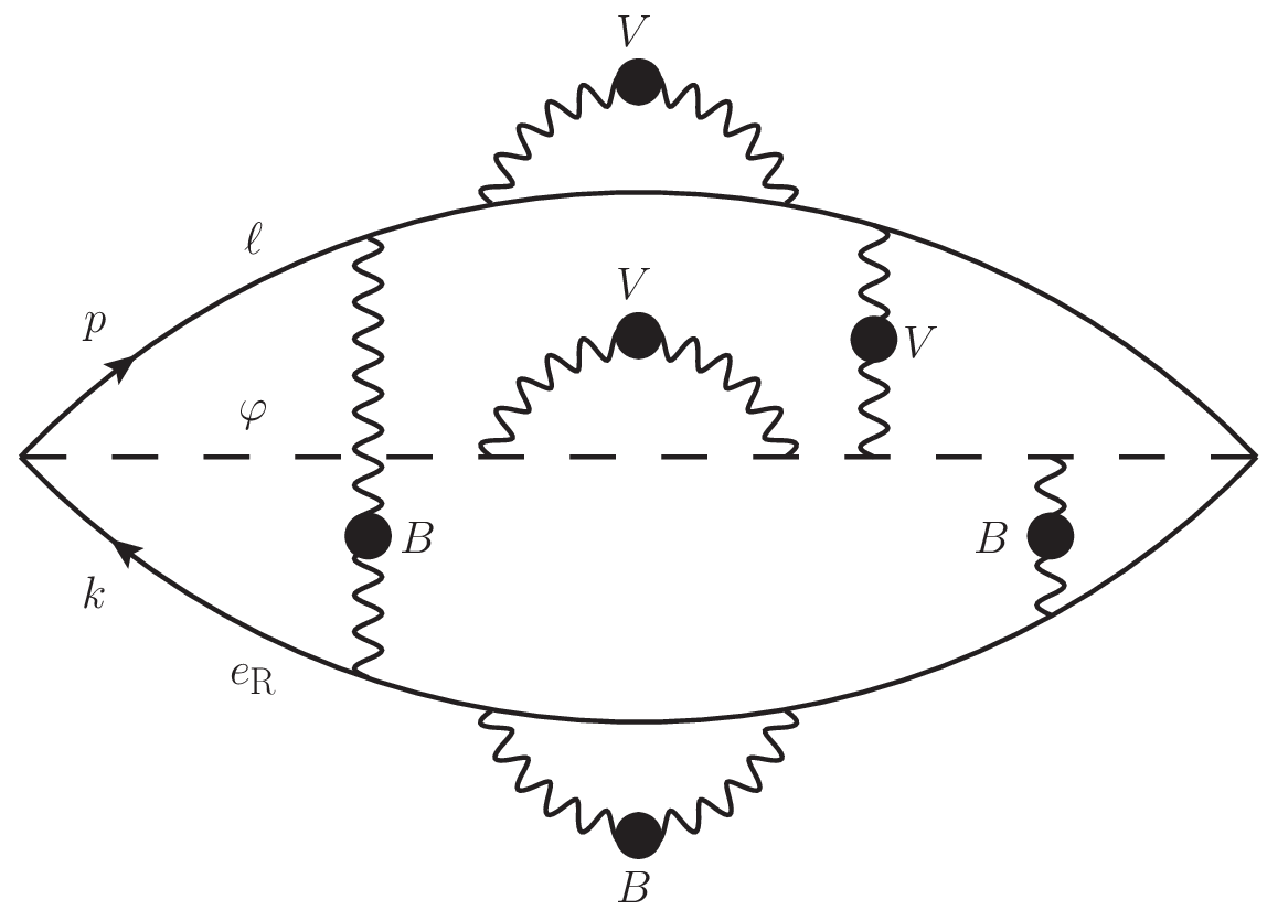
Now we include the effect of multiple scattering mediated by soft gauge bosons, as sketched in figure 2.⁶⁶ 6 The range of the gauge interactions is one power of $g$ smaller than the mean free path of the fermions and the Higgs. Therefore crossed gauge bosons, rainbow self-energies, or gauge boson vertex corrections do not contribute at leading order . The result can again be described by (3.19), where $j$ now satisfies

	$\displaystyle\delta E({\bf p}_{\perp},{\bf k}_{\perp})\;j({\bf p}_{\perp},{\bf k}_{\perp})$	$\displaystyle-i\int\frac{d^{2}q_{\perp}}{(2\pi)^{2}}\Big\{\mathscr{C}({\bf q}_{\perp}^{2})\big[j({\bf p}_{\perp},{\bf k}_{\perp})-j({\bf p}_{\perp}-{\bf q}_{\perp},{\bf k}_{\perp})\big]$
	$\displaystyle{}+\mathscr{C}^{\prime}({\bf q}_{\perp}^{2})\Big(y_{\varphi}y_{\ell}\big[$	$\displaystyle j({\bf p}_{\perp},{\bf k}_{\perp})-j({\bf p}_{\perp}-{\bf q}_{\perp},{\bf k}_{\perp})\big]$
	$\displaystyle{}+y_{\ell}\,y_{e_{\rm R}}\big[$	$\displaystyle j({\bf p}_{\perp},{\bf k}_{\perp})-j({\bf p}_{\perp}-{\bf q}_{\perp},{\bf k}_{\perp}-{\bf q}_{\perp})\big]$
	$\displaystyle{}-y_{\varphi}\,y_{e_{\rm R}}\big[$	$\displaystyle j({\bf p}_{\perp},{\bf k}_{\perp})-j({\bf p}_{\perp},{\bf k}_{\perp}-{\bf q}_{\perp})\big]\Big)\Big\}=\frac{1}{2}\chi^{\dagger}({\bf k})\eta({\bf p}).$		(3.21)

Here ${\bf q}_{\perp}$ is the transverse momentum of an exchanged gauge boson. We have introduced

	$\displaystyle\mathscr{C}({\bf q}_{\perp}^{2})$	$\displaystyle\equiv\frac{3}{4}g^{2}T\left(\frac{1}{{\bf q}_{\perp}^{2}}-\frac{1}{{\bf q}_{\perp}^{2}+m_{\rm D}^{2}}\right),$		(3.22)
	$\displaystyle\mathscr{C}^{\prime}({\bf q}_{\perp}^{2})$	$\displaystyle\equiv{g^{\prime}}^{2}T\left(\frac{1}{{\bf q}_{\perp}^{2}}-\frac{1}{{\bf q}_{\perp}^{2}+{m_{\rm D}^{\prime}}^{2}}\right)$		(3.23)

with the Debye masses [26]

$\displaystyle m_{\rm D}^{2}=\frac{11}{6}g^{2}T^{2},\quad\quad{m_{\rm D}^{\prime}}^{2}=\frac{11}{6}{g^{\prime}}^{2}T^{2}.$

(3.24)

In the integral in (3.21) the terms containing $j({\bf p}_{\perp},{\bf k}_{\perp})$ correspond to self-energy insertions, which can be easily checked by an explicit calculation.⁷⁷ 7 Note that $y_{\varphi}y_{\ell}+y_{\ell}y_{e_{\rm R}}-y_{\varphi}y_{e_{\rm R}}=\left(y_{\varphi}^{2}+y_{\ell}^{2}+y_{e_{\rm R}}^{2}\right)/2$. The terms with $\mathscr{C}$ and $\mathscr{C}^{\prime}$ correspond to interactions mediated by $W$ or $B$ bosons, respectively. By themselves, the self-energies are infrared divergent due to the $1/{\bf q}_{\perp}^{2}$ term in $\mathscr{C}$ and $\mathscr{C}^{\prime}$. The subtracted terms in the square brackets in (3.21) correspond to gauge boson exchange between different particles and render the ${\bf q}_{\perp}$-integrals finite. The first two square brackets in (3.21) also appear in the computation of the production rate of ultrarelativistic sterile neutrinos [10]. The other two represent the exchange of weak hypercharge gauge bosons by the right-handed electrons. Replacing the integral in (3.21) by $0^{+}$, one neglects multiple soft scatterings and one recovers the equation (3.20) describing Higgs decay.

Thanks to three-dimensional rotational invariance, the solution to (3.21) can be found as a function of a single transverse momentum [27],

$\displaystyle j({\bf p}_{\perp},{\bf k}_{\perp})=J({\bf P}),$

(3.25)

with

	$\displaystyle{\bf P}\equiv x_{k}{\bf p}_{\perp}$	$\displaystyle-x_{p}{\bf k}_{\perp},$		(3.26)
	$\displaystyle x_{k}\equiv\frac{k_{\parallel}}{p_{\parallel}-k_{\parallel}},\quad$	$\displaystyle\quad x_{p}\equiv\frac{p_{\parallel}}{p_{\parallel}-k_{\parallel}}.$		(3.27)

In fact, (3.17) now takes the simple form

$\displaystyle\delta E=\beta\left({\bf P}^{2}+M^{2}\right)$

(3.28)

with

$\displaystyle\beta$

$\displaystyle\equiv\frac{p_{\parallel}-k_{\parallel}}{2p_{\parallel}k_{\parallel}},$

(3.29)

and

$\displaystyle M^{2}$

$\displaystyle\equiv\beta^{-1}\left[\frac{m_{e_{\rm R}}^{2}}{2k_{\parallel}}-\frac{m_{\ell}^{2}}{2p_{\parallel}}-\frac{m_{\varphi}^{2}}{2(k_{\parallel}-p_{\parallel})}\right].$

(3.30)

The right-hand side of (3.21) turns into

$\displaystyle\frac{1}{2}\chi^{\dagger}({\bf k})\eta({\bf p})=-\frac{\beta}{2}\left(P_{x}-iP_{y}\right).$

(3.31)

The function $J({\bf P})$ can be expressed as

$\displaystyle J({\bf P})=\frac{i\beta}{4}\left[f_{x}({\bf P})-if_{y}({\bf P})\right],$

(3.32)

where the two-component vector ${\bf f}$ is a solution to

	$\displaystyle-i\delta E\;{\bf f}({\bf P})-\int\frac{d^{2}q_{\perp}}{(2\pi)^{2}}\Big\{\mathscr{C}({\bf q}_{\perp}^{2})\big[$	$\displaystyle{\bf f}({\bf P})-{\bf f}({\bf P}-x_{k}{\bf q}_{\perp})\big]$
	$\displaystyle{}+\mathscr{C}^{\prime}({\bf q}_{\perp}^{2})\Big(y_{\varphi}y_{\ell}\big[$	$\displaystyle{\bf f}({\bf P})-{\bf f}({\bf P}-x_{k}{\bf q}_{\perp})\big]$
	$\displaystyle{}+y_{\ell}\,y_{e_{\rm R}}\big[$	$\displaystyle{\bf f}({\bf P})-{\bf f}({\bf P}+{\bf q}_{\perp})\big]$
	$\displaystyle{}-y_{\varphi}\,y_{e_{\rm R}}\big[$	$\displaystyle{\bf f}({\bf P})-{\bf f}({\bf P}+x_{p}{\bf q}_{\perp})\big]\Big)\Big\}=2{\bf P}.$		(3.33)

This is the same integral equation as in [10] (with the appropriate hypercharge assignments), but with two additional terms representing the gauge interaction of right-handed electrons.

Now we choose the unit vector ${\bf v}$ in the direction of ${\bf k}$. Using ${\bf f}({\bf P})\propto{\bf P}$ and integrating over the transverse momentum ${\bf k}_{\perp}$, we obtain

$\displaystyle\Gamma^{\rm LPM}=\frac{h_{e}^{2}}{8\pi^{3}}\int\limits_{0}^{\infty}\!dk\!\int\limits_{-\infty}^{\infty}\!\!dp_{\parallel}\,\frac{\left(p_{\parallel}-k\right)^{3}}{p_{\parallel}^{2}k^{2}}\mathscr{F}(p_{\parallel},k)\;{\rm Re}\!\int\frac{d^{2}P}{(2\pi)^{2}}{\bf P}\cdot{\bf f}({\bf P})$

(3.34)

for the rate coefficient. We solve (3.33) using the algorithm described in [10] and numerically integrate (3.34) (see appendix B).

We first consider the case that the exchanged particles have hard momenta. Then the equilibration rate can be determined via the Boltzmann equation [28, 29]. We can write the time derivative of the $L_{e\rm R}$ density as

$\displaystyle\dot{n}_{L_{e\rm R}}=\int_{\bf k}\frac{\partial}{\partial t}\left[f_{{\bf k}}-\bar{f}_{{\bf k}}\right]$

(4.1)

where $f_{{\bf k}}$ and $\bar{f}_{{\bf k}}$ are the occupation numbers of right-handed electrons and positrons. We replace the time derivatives on the right-hand side by the collision term for $2\to 2$ particle scattering. It contains the occupancies of the participating particles in the form

$\displaystyle f_{1}f_{2}[1\pm f_{3}][1-f_{{\bf k}}]-[1\pm f_{1}][1\pm f_{2}]f_{3}f_{{\bf k}},$

(4.2)

corresponding to gain and loss term. The upper and lower signs are for bosons and fermions, respectively.

All Standard Model particles are in kinetic equilibrium due to their gauge interactions. Therefore their occupancies are determined by the temperature and by the chemical potentials of the slowly varying charges and of the strictly conserved ones. To compute $\Gamma$ at lowest order in chemical potentials, we can put all chemical potentials except $\mu_{e_{\rm R}}$ equal to zero. For the occupancy of right-handed electrons we can therefore write

$\displaystyle f_{{\bf k}}=f_{\rm F}(k^{0}-\mu_{e_{\rm R}})$

(4.3)

with $k^{0}=|{\bf k}|$, $\mu_{e_{\rm R}}=\mu_{L_{e\rm R}}$, and for the other Standard Model particles

$\displaystyle f_{i}=f_{\rm B,F}(p_{i}^{0}).$

(4.4)

In thermal equilibrium the gain and the loss term cancel,

$\displaystyle f_{1}f_{2}[1\pm f_{3}][1-f_{{\rm F}}(k^{0})]-[1\pm f_{1}][1\pm f_{2}]f_{3}f_{{\rm F}}(k^{0})=0,$

(4.5)

so that the collision term vanishes. Expanding to first order in $\mu_{e_{\rm R}}$ and making use of (4.5) together with

$\displaystyle f^{\prime}_{\rm F}=-\frac{1}{T}f_{\rm F}[1-f_{\rm F}],$

(4.6)

the contribution to the rate coefficient becomes

	$\displaystyle\Gamma^{2\to 2,{\rm hard}}=\frac{2}{T}\sum\limits_{\rm processes}\int_{{{\bf k}},{{\bf p}}_{1},{{\bf p}}_{2},{{\bf p}}_{3}}\frac{\sum|\mathscr{M}|^{2}}{16p_{1}^{0}\,p_{2}^{0}\,p_{3}^{0}\,k^{0}}\,(2\pi)^{4}$	$\displaystyle\delta^{(4)}(p_{1}+p_{2}-p_{3}-k)$
		$\displaystyle f_{1}f_{2}[1\pm f_{3}][1-f_{\rm F}(k^{0})]\Big|_{\rm hard}.$		(4.7)

Both terms on the right-hand side of (4.1) give the same contribution which gives rise to the factor $2$.

One can write (4.7) in terms of the $e_{\rm R}$-production rate at vanishing $e_{\rm R}$-density,

$\displaystyle\Gamma^{2\to 2,{\rm hard}}=\frac{2}{T}\int_{{\bf k}}\left[1-f_{\rm F}(k^{0})\right](2\pi)^{3}\left.\frac{dn_{e_{\rm R}}}{dtd^{3}k}\right|_{n_{e_{\rm R}}=0,\,{\rm hard}},$

(4.8)

which is closely related to the production rate of sterile neutrinos computed in [9]. The difference between the two processes is that the sterile neutrinos have no Standard Model gauge interactions, and therefore do not interact once they are produced (at LO in their Yukawa couplings). In contrast, the right-handed electrons carry weak hypercharge. Scatterings mediated by soft hypercharge gauge bosons contribute to the LO rate, as discussed in section 3. However for the $2\to 2$ scattering of hard particles the soft scattering is a higher order effect and can be neglected here.

The diagrams contributing to the ${e_{\rm R}}$-production are shown in figure 3. The matrix elements for the processes with quarks and $W$ bosons can be read off from [9] by setting $g^{\prime}\to 0$,

	$\displaystyle\text{quarks}:$	$\displaystyle\qquad\Sigma|\mathscr{M}|^{2}=6\,h_{t}^{2}\,h_{e}^{2},$		(4.9)
	$\displaystyle W\overline{\varphi}\rightarrow\overline{\ell}e_{\rm R}:$	$\displaystyle\qquad\Sigma|\mathscr{M}|^{2}=3g^{2}\,h_{e}^{2}\,\frac{u}{t},$		(4.10)
	$\displaystyle W\ell\rightarrow\varphi e_{\rm R}:$	$\displaystyle\qquad\Sigma|\mathscr{M}|^{2}=3g^{2}\,h_{e}^{2}\,\frac{-u}{s},$		(4.11)
	$\displaystyle\ell\overline{\varphi}\rightarrow We_{\rm R}:$	$\displaystyle\qquad\Sigma|\mathscr{M}|^{2}=3g^{2}\,h_{e}^{2}\,\frac{s}{-t},$		(4.12)

where (4.9) holds for any of the processes $\overline{t}Q_{3}\rightarrow\ell e_{\rm R},\,Q_{3}\ell\rightarrow te_{\rm R},\,\overline{t}\ell\rightarrow\overline{Q}_{3}e_{\rm R}$. For the processes with hypercharge gauge bosons we find

	$\displaystyle B\overline{\varphi}\rightarrow\overline{\ell}e_{\rm R}:$	$\displaystyle\qquad\Sigma|\mathscr{M}|^{2}={g^{\prime}}^{2}\,h_{e}^{2}\,\left[4+\frac{u}{t}+\frac{4t}{u}\right],$		(4.13)
	$\displaystyle B\ell\rightarrow\varphi e_{\rm R}:$	$\displaystyle\qquad\Sigma|\mathscr{M}|^{2}={g^{\prime}}^{2}\,h_{e}^{2}\,\left[-4+\frac{-u}{s}+\frac{4s}{-u}\right],$		(4.14)
	$\displaystyle\ell\overline{\varphi}\rightarrow Be_{\rm R}:$	$\displaystyle\qquad\Sigma|\mathscr{M}|^{2}={g^{\prime}}^{2}\,h_{e}^{2}\,\left[-4+\frac{s}{-t}+\frac{4(-t)}{s}\right].$		(4.15)

Here we have summed over polarizations, color and weak isospin. The Boltzmann equation can now be integrated as in [9], with some additional integrals due to the terms containing a factor $4$ in (4.13) through (4.15). We rewrite the contributions proportional to $1/(-u)$ as a process proportional to $1/(-t)$ by interchanging the incoming particles, which may change the statistics of particles 1 and 2.

In the integrals describing lepton exchange in $t$-channel we need to handle the infrared divergence appearing when the momentum of the exchanged lepton becomes small. We proceed as in [9] by introducing a transverse momentum cutoff $q_{\rm cut}$ for the exchanged particle with $gT\ll q_{\rm cut}\ll T$. We isolate the piece which is singular for $q_{\rm cut}\to 0$ and integrate it analytically. Its logarithmic $q_{\rm cut}$ dependence drops out when combined with the soft contribution (see section 4.2) which includes only transverse momenta less than $q_{\rm cut}$. The remaining finite integral is then computed numerically.

The soft contribution is obtained from the retarded correlator using (2.7), where either of the lepton propagators is HTL resummed. The corresponding diagrams are shown in figure 4. A straightforward computation in imaginary time, in which we make use of the sum rule found in [9], and analytic continuation to real frequency leads to

$\displaystyle\Gamma^{{\rm soft}}=\frac{h_{e}^{2}\,T}{64\,\pi}\,\left[m_{\ell}^{2}\log\left(\frac{q_{\rm cut}}{m_{\ell}}\right)+m_{e_{\rm R}}^{2}\log\left(\frac{q_{\rm cut}}{m_{e_{\rm R}}}\right)\right].$

(4.16)

Adding the hard singular and finite as well as the soft contributions, $q_{\rm cut}$ drops out, and the contribution from $2\to 2$ scatterings to the rate coefficient $\Gamma$ is finite. Evaluating the remaining integrals numerically, we find

	$\displaystyle\Gamma^{2\rightarrow 2}=\frac{h_{e}^{2}\,T^{3}}{2048\,\pi}\Bigg\{h_{t}^{2}c_{t}+\left(3g^{2}+{g^{\prime}}^{2}\right)$	$\displaystyle\left[c_{\ell}+\log\frac{1}{3g^{2}+{g^{\prime}}^{2}}\right]$
	$\displaystyle{}+\,4{g^{\prime}}^{2}$	$\displaystyle\left[c_{e_{\rm R}}+\log\frac{1}{4{g^{\prime}}^{2}}\right]\Bigg\}$		(4.17)

with

$\displaystyle c_{t}=2.82,\quad\quad\quad c_{\ell}=3.52,\quad\quad\quad c_{e_{\rm R}}=2.69.$

(4.18)

References

- [1] B. A. Campbell, S. Davidson, J. R. Ellis and K. A. Olive, On the baryon, lepton flavor and right-handed electron asymmetries of the universe, Phys. Lett. B297 (1992) 118–124, [hep-ph/9302221].
- [2] J. M. Cline, K. Kainulainen and K. A. Olive, Protecting the primordial baryon asymmetry from erasure by sphalerons, Phys. Rev. D49 (1994) 6394–6409, [hep-ph/9401208].
- [3] E. K. Akhmedov, V. A. Rubakov and A. Yu. Smirnov, Baryogenesis via neutrino oscillations, Phys. Rev. Lett. 81 (1998) 1359–1362, [hep-ph/9803255].
- [4] T. Asaka and M. Shaposhnikov, The nuMSM, dark matter and baryon asymmetry of the universe, Phys. Lett. B620 (2005) 17–26, [hep-ph/0505013].
- [5] M. Joyce and M. E. Shaposhnikov, Primordial magnetic fields, right-handed electrons, and the Abelian anomaly, Phys. Rev. Lett. 79 (1997) 1193–1196, [astro-ph/9703005].
- [6] M. Beneke, B. Garbrecht, C. Fidler, M. Herranen and P. Schwaller, Flavoured Leptogenesis in the CTP Formalism, Nucl. Phys. B843 (2011) 177–212, [1007.4783].
- [7] B. Garbrecht, F. Glowna and P. Schwaller, Scattering Rates For Leptogenesis: Damping of Lepton Flavour Coherence and Production of Singlet Neutrinos, Nucl. Phys. B877 (2013) 1–35, [1303.5498].
- [8] D. G. Figueroa and M. Shaposhnikov, Anomalous non-conservation of fermion/chiral number in Abelian gauge theories at finite temperature, JHEP 04 (2018) 026, [1707.09967].
- [9] D. Besak and D. Bodeker, Thermal production of ultrarelativistic right-handed neutrinos: Complete leading-order results, JCAP 1203 (2012) 029, [1202.1288].
- [10] A. Anisimov, D. Besak and D. Bodeker, Thermal production of relativistic Majorana neutrinos: Strong enhancement by multiple soft scattering, JCAP 1103 (2011) 042, [1012.3784].
- [11] L. D. Landau and I. Pomeranchuk, Limits of applicability of the theory of bremsstrahlung electrons and pair production at high-energies, Dokl. Akad. Nauk Ser. Fiz. 92 (1953) 535–536.
- [12] L. D. Landau and I. Pomeranchuk, Electron cascade process at very high-energies, Dokl. Akad. Nauk Ser. Fiz. 92 (1953) 735–738.
- [13] A. B. Migdal, Bremsstrahlung and pair production in condensed media at high-energies, Phys. Rev. 103 (1956) 1811–1820.
- [14] R. Baier, Y. L. Dokshitzer, A. H. Mueller, S. Peigne and D. Schiff, Radiative energy loss of high-energy quarks and gluons in a finite volume quark - gluon plasma, Nucl. Phys. B483 (1997) 291–320, [hep-ph/9607355].
- [15] B. G. Zakharov, Fully quantum treatment of the Landau-Pomeranchuk-Migdal effect in QED and QCD, JETP Lett. 63 (1996) 952–957, [hep-ph/9607440].
- [16] P. B. Arnold, G. D. Moore and L. G. Yaffe, Photon and gluon emission in relativistic plasmas, JHEP 06 (2002) 030, [hep-ph/0204343].
- [17] D. Bodeker and M. Laine, Kubo relations and radiative corrections for lepton number washout, JCAP 1405 (2014) 041, [1403.2755].
- [18] D. Bodeker and M. Sangel, Lepton asymmetry rate from quantum field theory: NLO in the hierarchical limit, JCAP 1706 (2017) 052, [1702.02155].
- [19] S. Yu. Khlebnikov and M. E. Shaposhnikov, Melting of the Higgs vacuum: Conserved numbers at high temperature, Phys. Lett. B387 (1996) 817–822, [hep-ph/9607386].
- [20] J. Ghiglieri and M. Laine, GeV-scale hot sterile neutrino oscillations: a derivation of evolution equations, JHEP 05 (2017) 132, [1703.06087].
- [21] H. A. Weldon, Effective Fermion Masses of Order gT in High Temperature Gauge Theories with Exact Chiral Invariance, Phys. Rev. D26 (1982) 2789.
- [22] P. B. Arnold, G. D. Moore and L. G. Yaffe, Photon emission from ultrarelativistic plasmas, JHEP 11 (2001) 057, [hep-ph/0109064].
- [23] P. Aurenche, F. Gelis, G. D. Moore and H. Zaraket, Landau-Pomeranchuk-Migdal resummation for dilepton production, JHEP 12 (2002) 006, [hep-ph/0211036].
- [24] R. Baier, Y. L. Dokshitzer, A. H. Mueller, S. Peigne and D. Schiff, Radiative energy loss and p(T) broadening of high-energy partons in nuclei, Nucl. Phys. B484 (1997) 265–282, [hep-ph/9608322].
- [25] B. G. Zakharov, Radiative energy loss of high-energy quarks in finite size nuclear matter and quark - gluon plasma, JETP Lett. 65 (1997) 615–620, [hep-ph/9704255].
- [26] M. E. Carrington, The Effective potential at finite temperature in the Standard Model, Phys. Rev. D45 (1992) 2933–2944.
- [27] P. Arnold and S. Iqbal, The LPM effect in sequential bremsstrahlung, JHEP 04 (2015) 070, [1501.04964].
- [28] H. A. Weldon, Simple Rules for Discontinuities in Finite Temperature Field Theory, Phys. Rev. D28 (1983) 2007.
- [29] M. Laine, Thermal 2-loop master spectral function at finite momentum, JHEP 05 (2013) 083, [1304.0202].
- [30] P. Hernández, M. Kekic, J. López-Pavón, J. Racker and J. Salvado, Testable Baryogenesis in Seesaw Models, JHEP 08 (2016) 157, [1606.06719].
- [31] J. Ghiglieri and M. Laine, GeV-scale hot sterile neutrino oscillations: a numerical solution, JHEP 02 (2018) 078, [1711.08469].
- [32] K. Kamada and A. J. Long, Baryogenesis from decaying magnetic helicity, Phys. Rev. D94 (2016) 063501, [1606.08891].
- [33] A. J. Long, E. Sabancilar and T. Vachaspati, Leptogenesis and Primordial Magnetic Fields, JCAP 1402 (2014) 036, [1309.2315].
- [34] D. T. Son and P. Surowka, Hydrodynamics with Triangle Anomalies, Phys. Rev. Lett. 103 (2009) 191601, [0906.5044].
- [35] P. B. Arnold, G. D. Moore and L. G. Yaffe, Transport coefficients in high temperature gauge theories. 1. Leading log results, JHEP 11 (2000) 001, [hep-ph/0010177].