A level-set multigrid technique for nonlinear diffusion in the numerical simulation of marble degradation under chemical pollutants
Abstract
Having in mind the modelling of marble degradation under chemical pollutants, e.g. the sulfation process, we consider governing nonlinear diffusion equations and their numerical approximation. The space domain of a computation is the pristine marble object. In order to accurately discretize it while maintaining the simplicity of finite difference discretizations, the domain is described using a level-set technique. A uniform Cartesian grid is laid over a box containing the domain, but the solution is defined and updated only in the grid nodes that lie inside the domain, the level-set being employed to select them and to impose accurately the boundary conditions. We use a Crank-Nicolson scheme in time, while for the space variables the discretization is performed by a standard Finite-Difference scheme for grid points inside the domain and by a ghost-cell technique on the ghost points (by using boundary conditions). The solution of the large nonlinear system is obtained by a Newton-Raphson procedure and a tailored multigrid technique is developed for the inner linear solvers. The numerical results, which are very satisfactory in terms of reconstruction quality and of computational efficiency, are presented and discussed at the end of the paper.
1 Introduction
Quantitative forecasts of damage by gaseous pollutants to monuments are becoming more and more important, since they allow to schedule monitoring, preservation and, when needed, restoration activities in the management of cultural heritage [22]. Phenomena involving chemical reactions of the constitutive material of a work of art with chemicals in the surrounding environment have long been recognized very important for the damage to cultural heritage sites. In a recent review of the related mathematical models [51], the employment of models based on partial differential equations has been advocated for the next generation of models with regulatory powers.
Differential models in this field typically involve a, possibly nonlinear, diffusion term describing the penetration of the gas in the bulk material, coupled with reaction terms modelling the chemistry of the interaction. A typical example is the sulfation process that turns marble into gypsum, for which a model was proposed in [4]. More recent models include the effects of the Darcy velocity [2], of the surface rugosity [8]; a kinetic approach to the derivations of the models of sulfation was proposed in [1]. More complex models including free boundaries can take into account the swelling of the material [15] or treat appropriately the heterogeneity of the crust layer [46]. Modelling of layered material with moving interfaces has been exploited also for copper corrosion in [14].
In this paper we focus on the model of [4], since it is quite simple but yet contains the more relevant numerical difficulties. Previous numerical work on this model have considered the one-dimensional version of the model [33] or Cartesian grids in two space dimensions [52]. Of course this kind of meshes cannot stand one of the main difficulties of this kind of computations, which is the accurate discretization of the domain. This is quite relevant, since, despite the simplicity of the numerical techniques in [52], the computational model have shown the importance of two-dimensional effects near corners and other sharp features of the domain. In a real case should coincide with the pristine work of art and only rarely this can be accurately represented on a Cartesian grid.
One of the simplest methods to overcome this difficulty consists of approximating by small cuboids, whose size and shape are eventually adapted close to the boundary of in such as way that the most external corners lie on the boundary. This approach is adopted by the Shortley-Weller discretization [54], providing the simplest approach falling under the class of boundary-fitted grid methods, where the grid is suitably adapted to the boundary of the domain. Although the Shortley-Weller discretization is designed for Dirichlet boundary conditions and can be highly accurate for the solution and its gradient [53], the extension to Neumann boundary conditions is not straightforward.
More accurate and well-known boundary-fitted methods are represented by the Finite Element Methods (FEM), successfully adopted in several scientific contexts (e.g., [10, 11, 36, 6, 9, 41, 38, 27, 37, 23]). However, fitting the mesh to a complex domain with several corners or highly variable curvature might be computationally demanding. Another alternative for working with a Cartesian structure is furnished by the Isogeometric approach, adopted for example in [57, 40], where an evident difficulty is given by the need of using several patches when the domain is complicate and of course this is a concrete possibility when treating the degradation e.g. of a statue from our cultural heritage.
For all these reasons, the mathematical models proposed in this paper, where the domain coincides with the realistic monument with its sharp features, would be more efficiently solved by numerical approaches where the boundary is embedded in a steady Cartesian grid and implicitly described by a level-set function. Another advantage of this approach is that it would be easier to generalize the methods to the case of evolving boundaries or the presence of internal interfaces, advocated by the more modern models in [15, 46, 14].
The first methods falling under this category were the Immersed Boundary Method [50] and the Immersed Interface Methods [43], proposed to model blood flows in the heart.
More recent numerical approaches to discretise partial differential equations on complex domains in a Cartesian grid are the Ghost-Fluid Methods proposed in [29, 34, 35, 45], where the solution and the Dirichlet boundary condition are extrapolated to define ghost values outside the domain in order to maintain a standard discretization stencil on internal grid points without compromising the overall accuracy order.
An improved version that accounts for Neumann boundary conditions was proposed by Coco and Russo in [19, 21, 18]. In this method a high order accuracy is achieved not only for the solution but also for the gradient of the solution.
Other recent methods for Neumann boundary conditions were proposed in [39], while the accuracy order for the gradient of the solution has been improved in [7].
Among the other unfitted-boundary approaches, we mention the matched interface (MIB) method [58], the Immersed Finite Volume Methods (IFVM) [47, 28], the arbitrary Lagrangian Eulerian method (ALE) [30, 26], and the penalization methods [42, 3, 12].
Within this paper we consider a novel numerical technique for the approximation of nonlinear (possibly degenerate) parabolic equations, which relies on the finite difference discretization and efficient solvers of [52, 24, 25] and on the level-set domain description and handling of boundary conditions of [19]. As in [52], the time discretization is the implicit Crank-Nicolson, a large nonlinear system at each time step is solved by a Newton-Raphson procedure, with a tailored multigrid technique for the linear systems. The spatial discretization is achieved by finite differences on a uniform Cartesian grid and, in the bulk of the domain, the numerical scheme is the same as in [24]. However, here, the domain can be of arbitrary shape and is implicitly defined by , where the level-set function is known at least at the grid nodes. The grid nodes are defined, according to , as internal (those inside ), ghosts (first layer of points around the internal ones) and external. The method of [24] is applied only on the internal grid points. In order to close the method, the resulting nonlinear system of equations is augmented, as in [19], by the equations expressing the fulfillment of the boundary conditions on in terms of the ghost values and of their first internal neighbour points. The resulting system is then solved by Newton-Raphson and the special smoothing technique of [19] is employed in the multigrid linear solver.
The outline of the paper is the following. In §2 we introduce the mathematical model. The numerical method is discusses in §3, discussing the details of the time discretization in §3.1, the space discretization in §3.2 and §3.3, the Newton-Raphson solver in §3.4 and the multigrid method in §3.5. The numerical tests of §4 include accuracy and efficiency tests, as well as examples of application to nontrivial geometries §4.3. Finally, the main conclusions of the paper and perspectives for future work are discussed in §5.
The numerical results, which are very satisfactory both from the viewpoint of the reconstruction quality and of the computational efficiency, are presented and discussed at the end of the paper.
2 Mathematical Model
Here we recall briefly the model of marble sulfation introduced in [4], referring the reader to the original paper for the details and more comprehensive study of the properties of the solutions. In [4], the authors consider the (simplified) chemical reaction
to account for the transformation of of the marble stone into (gypsum), that is triggered in a moist atmosphere by the availability of at the marble surface and inside the pores of the stone.
Letting represent the pristine marble piece, the equations governing the process of marble sulfation are:
| (1) |
where represents the marble concentration, initially set to , and is the gas concentration, initially set to . The evolution equations (1) are characterized by a diffusion term for , that is nonlinear since the diffusion coefficient depends on , and by reaction terms coupling the two variables. Boundary conditions are of Dirichlet type and impose a value of on the boundary of , representing the pollution level of the surrounding air. It is assumed that, the gypsum concentration is and so, as time goes by, the calcium carbonate concentration is reduced from the initial value , as is progressively replaced by a gypsum crust that forms on the outer shell of the monument and whose thickness and evolution are of interest to the managers of cultural heritage.
The time evolution is described by the diffusion term in the gas equation and by the reaction terms in both differential equations. The porosity of the material controls the diffusion of the gas in the pores of the marble. Since marble and gypsum have different porosities, is not a constant but a function of the , making the diffusion equation a nonlinear one. For simplicity, as in [4], we assume that
We point out that more complex relations may be employed, since our method does not rely strongly on the linearity of the above relation.
The third equation is the boundary condition for and describes the condition surrounding the work of art. We assume for simplicity a Dirichlet boundary condition, although the method proposed in this paper can be extended to more sophisticated boundary conditions on fluxes such as in the free boundary model proposed in 1D in [15]. We observe that no boundary condition is needed for , since the second equation of (1) does not involve spatial derivatives. Last two equations represent the initial conditions.
Although the model can be cast in higher dimensions, in this paper we focus on the 2D case for simplicity, since it contains already the main difficulties of the full 3D model. Let be the computational domain, the domain representing the marble monument, the boundary of the domain. The numerical method will consider a regular grid in and a level-set function defined on the grid will be used both to detect the grid points inside and to describe the exact location and outward normal for the boundary of .
3 Numerical method
3.1 Time discretization
Equations (1) are discretized in time using the second order accurate Crank-Nicolson scheme
| (2) |
where
are the differential operators representing the right-hand side of (1), while and are functions of space only and represent approximations of the solutions and , respectively, at time , for (with ).
3.2 Level-set function
The domain is represented by an auxiliary level-set function :
Level-set methods have been firstly proposed by Sethian and Osher [49] and widely used since then to solve PDEs in complex-shaped geometries and moving domains [48]. The level-set function is convenient to gather geometric information, such as the outward unit normal vector and the curvature of the boundary :
| (3) |
Among the infinite level-set functions that can describe a domain , the signed distance function has the advantage to maintain a stable algorithm since steep or shallow gradients are avoided. If the signed distance function is not available, it can be approximated from a generic level-set function by approximating the solution of the following PDE up to steady state (reinitialization step):
where is a fictitious time parameter [48]. The numerical methods proposed in this paper are designed for generic level-set function and therefore do not rely on the availability of the signed-distance function.
We observe that in real applications the level-set function must be derived from image data, usually starting from a cloud of points given by a 3D laser scanner. The level-set function can be obtained as follows. First, a provisional level-set function is defined by setting inside the domain and outside the domain, introducing a stepwise effects on the boundary. Then, the level-set function is slightly diffused (few iterations of diffusion equation), and the stepwise effects on the boundary disappear without affecting the important features of the monument. In this paper, we adopt the simplified 2D version of this technique to pixelated black and white images representing a woman head profile, a shark and a necklace (see §4.3).
3.3 Spatial discretization
Discretization in space is performed by a standard finite-difference scheme for the grid points lying inside the domain and by a ghost-cell technique on the ghost points (to impose high order accurate boundary conditions).
Let be the computational domain and let be the number of intervals in each direction. We call the spatial step. Observe that we are assuming for simplicity that , although the method can be easily generalised to the case .
The set of grid points is . Let be the discrete counterpart of .
We say that a grid point is a ghost point if and only if both of the following conditions are satisfied:
| (4) |
In other words, a ghost point is a grid point that is outside the domain and that has one of its four neighbour grid points inside . We call the set of ghost points (see Fig. 2).
Let and be the sets of inside indices and ghost indices, respectively, and and be their cardinalities.
We aim at approximating the solution in for any time step. Therefore, the numerical solution at each time step is expressed by a vector , whose components are and , with varying in .
The components of are ordered by choosing a mapping
| (5) |
For the purpose of describing the numerical method, we order all variables before the ones, i.e. . Of course, the actual layout of the vector in the computer memory will be chosen to achieve optimal efficiency, e.g. like .
In order to compute from , a system of nonlinear equations in unknowns must be solved at each time step. The nonlinear system is obtained as follows. The nonlinear equations related to inside grid points are obtained by discretizing the first two equations of (2) on inside grid points using the standard five-point stencil (Fig. (2)) finite-difference scheme:
| (6) |
| (7) |
where
and is the set of four neighbouring index pairs for , namely:
Eq. (7) is discretized also on ghost points (provided that the initial conditions for and are extrapolated outside the domain with second order accuracy, using for example the extrapolation technique proposed in [5]), leading to additional nonlinear equations. The remaining equations are obtained by enforcing the boundary condition for on
| (8) |
using a ghost point extrapolation technique that was already successfully adopted in other contexts (elliptic [19, 21, 18, 17, 16] and hyperbolic [13, 20] equations) and described as follows. Let be a ghost point and be the approximated outward unit normal vector computed by a central finite-difference discretization of Eq. (3):
| (9) |
Let be the nine-point stencil in the upwind direction with respect to . More precisely,
where and , with or if or , respectively, and (conventionally) . Since this nine-point stencil is taken in the upwind direction with respect to the normal , it can be easily proven that , provided that the grid is sufficiently fine (i.e. is sufficiently small).
The linear equations are obtained by prescribing the boundary condition (8) on , where is the normal projection of onto , obtained by the following algorithm (see Fig. 4):
- •
compute (we have provided that the grid is sufficiently fine, i.e. is sufficiently small);
- •
apply the bisection method to solve in the unknown (with the tolerance criterion: ), where is a biquadratic interpolation of on the stencil ;
- •
compute .
Finally, the linear equations are:
| (10) |
where is the biquadratic interpolations of on the stencil .
We observe that when only Dirichlet boundary conditions are considered, other boundary discretization approaches can result more efficient and easier to implement, such as Shortley-Weller methods [54] or the symmetric positive-definite discretization proposed in [34]. However, the method proposed here is robust for all types of boundary conditions (Dirichlet, Neumann, Robin, mixed) and an extension to Neumann boundary conditions is proposed in §3.6 and tested in §4.1 (Test 1N and Test 2N), making the approach suitable for an extension to more complex models of monument conservation, such as the free boundary models proposed in 1D in [15], where a non-homogenous free boundary conditions involving fluxes is proposed to account for the swelling of the external gypsum layer, The 3D implementation is currently under investigation.
3.4 Newton-Raphson method
Eqs. (6), (7), (10) constitute the system of nonlinear equations that we need to solve in order to advance in time from to . Let be an operator such that the nonlinear system ((6), (7), (10)) can be represented by . This system is solved by the Newton-Raphson method, i.e. by the following iterative scheme:
- 1.
take the initial guess ;
- 2.
for , repeat the steps:
- (a)
solve the linear system
(11) where is the Jacobian matrix of ;
- (b)
update the current guess .
until a suitable tolerance is reached, e.g.:
- (a)
The Jacobian matrix can be represented in the compact form
| (12) |
where are the four matrices detailed below. Note that (12) describes the logical structure of the Jacobian matrix, and that its actual layout in the computer memory may be different and will match the layout chosen for the vectors .
We represent the rows of a matrix by stencils in the following way: we say that the stencil
represents the -th row of a matrix , with , if for any we have that
We have boxed the central element to emphasize that this element is on the main diagonal of the matrix , i.e. . Sometimes (in particular for ghost points) it may be easier to have the element of the main diagonal not necessarily at the center of the stencil. Therefore, we use for instance the stencil
if we want to represent the -th row of as:
Representation of the matrix .
Using this notation, if the -th row of is:
| (13) |
Let and , (see Fig. 4 and Eq. (9)). Referring to Fig. 5, observe that the three coefficients
| (14) |
are the 1D quadratic interpolation coefficients on for grid points , , , respectively, with .
The 2D biquadratic interpolation (15) is obtained as dimension by dimension quadratic interpolations. Therefore, the -th row of is represented by
| (15) |
with
The other three possible cases , and are obtained similarly. Observe that the coefficients of the other three cases are the same as in (15), but in a different order, and that the boxed coefficient (i.e. the coefficient that will populate the main diagonal of the matrix) has the same expression in all cases.
Representation of the matrix .
The -th row of is
| (16) |
if , or a null row if .
Representation of the matrix .
The -th row of is
| (17) |
both if or .
Representation of the matrix .
The -th row of is represented by
| (18) |
both if or .
Summarizing, the four sub-matrices of the Jacobian matrix (12) can be represented in matrix form (see Eqs. (13), (15), (16), (17), (18)):
where , , , are four diagonal matrices, , are two penta-diagonal matrices, while is a nine-diagonal matrix that does not depend on and then can be precomputed at the beginning of the numerical simulation.
3.5 Multigrid method
The linear system (11) is solved by a multigrid tecnique, as described in this section. In particular, we will introduce the relaxation operator (§3.5.1) and the transfer (restriction and interpolation) operators (§3.5.2 and 3.5.3). The multigrid method can then be easily implemented from these operators (we refer the reader to any book on multigrid methods for a comprehensive presentation, such as [56]). In this paper we implement the cycle multigrid scheme and compare its convergence factor against the one predicted by the Local Fourier Analysis for cycle multigrid schemes in rectangular domains. Extensions to multigrid schemes more efficient than cycle such as Full-multigrid [56, Ch. 2.6] can be also easily implemented following the same approach proposed in this paper.
3.5.1 Relaxation operator
Let us write the linear system (11) as:
In order to have an efficient multigrid method, the relaxation operator must satisfy the smoothing property, i.e. the high frequency components of the defect should be dumped quickly after few relaxations, in such a way that the residual linear system is well represented on a coarser grid (see [56, Ch. 2.1]). Well known relaxation operators that satisfy the smoothing property for scalar elliptic equations are Gauss-Seidel and weighted-Jacobi (with ). It is known that the classical Gauss-Seidel scheme may underperform for systems of partial differential equations, where the collective Gauss-Seidel scheme is usually preferred ([56, Ch. 8]). In this paper we implement a collective Gauss-Seidel scheme, i.e. a linear system is solved at each internal grid point to update and simultaneously, while an appropriate relaxation is performed on ghost points ([19, 21, 18]). In detail, the relaxation scheme spans all . If , then and are updated as follows:
where and are the th components of the vectors and , respectively, and is the th row of the matrix (see Eqs. (13), (16), (17), (18)). We have denoted by and the current approximations of the Gauss-seidel iteration, i.e. they are vectors whose th component is defined by:
| (19) |
and
| (20) |
We observe that the classical (pointwise) Gauss-Seidel scheme can be obtained by replacing the matrix (20) with
| (21) |
If , then and are updated as follows:
| (22) |
where is the th row of the matrix (see Eqs. (15)). If we choose as in (21) to have a Gauss-Seidel iteration, i.e.
the relaxation scheme may not converge (we observe for example that rows (15) are not diagonally dominant). Following the idea proposed in [19, 21, 18], the parameter is chosen in such a way that a proper CFL condition is satisfied for the iterations (22). In particular, we want to ensure that the absolute value of the coefficient of in the right-hand side of (22) is smaller than one, i.e.
| (23) |
We choose a parameter that satisfies the condition (23) for any . This is achieved by: For practical purposes, we use
Finally, although in this paper we will use the lexicographic order of the map (5), more efficient (collective) Gauss-Seidel schemes for multigrid methods, such as Red-Black Gauss-Seidel, can be easily implemented.
3.5.2 Restriction operator
After pre-relaxation iterations (§3.5.1), we compute the defects and :
that will be restricted to the coarser grid (with spatial step ) by a suitable restriction operator :
We observe that the defect is discontinuous across the boundary, because the defect on is related to the internal equations, while its values on are referred to the boundary conditions. For this reason, the restriction of the internal equations must use values only from . (see [19]) To this purpose, the restriction operator is appropriately modified for internal grid points in the vicinity of . We recall the full-weighting restriction operator (see [56, Ch. 2.3.3]):
| (24) |
In general, by the stencil notation
| (25) |
we will denote the restriction operator defined by:
where only a finite number of coefficients is different from zero, and for some positive integer . A second order restriction is achieved with .
Following the same idea of [19, 21], we modify the restriction operator close to the boundary in order to disregard the values of the defects on ghost points (see Fig. 6 and [19, 21] for more details).
The restriction of the boundary condition is performed using the same idea, namely using only points outside the domain (i.e. either ghost points or inactive grid points), provided that the defect is firstly defined in the neighbouring inactive points by extrapolating the ghost value constantly along the normal direction to the boundary . This can be achieved by solving the transport equations
for a few steps of a fictitious time , (using for example Euler explicit method), where is the unit normal vector.
3.5.3 Interpolation operator
The defect equations
are solved recursively on the coarser grid (where are approximated in the coarser grid using the same technique as in the fine grid), and then the error is interpolated back to the finer grid:
Since errors and are continuous across the boundary, we can use values from both sides of the boundary in the same stencil and therefore we can adopt a standard linear interpolation operator for all points:
Finally, post-relaxation iterations (§3.5.1) are performed on the finer grid.
3.6 Neumann boundary conditions
In this section we extend the numerical approach to the case of Neumann boundary conditions for . The implementation of more sophisticated boundary conditions (Robin, mixed, etc.) will then be straightforward. We consider the Neumann boundary condition
instead of (8).
The spatial discretization (10) becomes:
| (26) |
where and are the the biquadratic interpolations of and , respectively, on the stencil . The -th row of when (Eq. (15)) is obtained by using the condition (26):
| (27) |
Since the coefficients of the 1D quadratic approximation of the first derivative on are (see Fig. 5)
| (28) |
for grid points , , , respectively, then the -th row of is represented by (from (27), see Fig. 4):
| (29) |
with
where the product operator means the product component-wise between the two matrices and the sum over all components (inner products between the two vector representations of the two matrices).
4 Numerical tests
In this section we confirm numerically the second order accuracy of the numerical method and we evaluate the efficiency of the multigrid approach. We choose the following parameters in Eq. (1) (see [52]):
| (31) |
We choose and we compute the numerical solution up to the final time . The W-cycle iteration scheme of the multigrid is performed with pre-relaxation, post-relaxation and with an grid as the coarsest grid.
4.1 Accuracy tests
In order to test the accuracy, we modify the numerical method to solve a more general problem than (1) by adding source terms :
We choose in such a way that the exact solutions are:
and then we compute the errors at time on the solutions
and on the gradients
where and are the numerical solutions and and are computed by central differences. We perform two tests. In Test 1, the domain is represented by a circle and the level-set function is:
| (32) |
In Test 2 the domain is represented by the union of a square and four circles centred on the vertices
| (33) |
where
The domains for Test 1 and Test 2 are represented in Fig. 7. and errors for the solutions and the gradients for Test 1 can be found in Table 1 (for ) and Table 2 (for ), and for Test 2 in Table 3 (for ) and Table 4 (for ). Bestfit lines in bilogarithmic plots for the errors versus can be found in Figs. 9 ( in Test 1), 9 ( in Test 1), 11 ( in Test 2) and 11 ( in Test 2). We repeat the two tests for the case of Neumann boundary conditions for as described in §3.6) (Test 1N and Test 2N) and present the results in Tables 5, 6, 7 and 8 and in Figures 13, 13, 15 and 15. We note that in all cases second order convergence is achieved.


| No. of points | error of | order | error of | order |
| 16 16 | 2.00 | - | 1.93 | - |
| 32 32 | 4.03 | 2.31 | 4.67 | 2.05 |
| 64 64 | 7.38 | 2.45 | 8.35 | 2.48 |
| 128 128 | 1.43 | 2.37 | 1.42 | 2.56 |
| 256 256 | 3.03 | 2.24 | 1.95 | 2.86 |
| No. of points | error of | order | error of | order |
| 16 16 | 1.20 | - | 1.30 | - |
| 32 32 | 2.88 | 2.06 | 3.25 | 2.00 |
| 64 64 | 7.03 | 2.03 | 8.13 | 2.00 |
| 128 128 | 1.73 | 2.02 | 2.03 | 2.00 |
| 256 256 | 4.30 | 2.01 | 5.08 | 2.00 |
| No. of points | error of | order | error of | order |
| 16 16 | 2.04 | - | 1.92 | - |
| 32 32 | 4.60 | 2.15 | 5.10 | 1.91 |
| 64 64 | 8.52 | 2.43 | 1.12 | 2.19 |
| 128 128 | 1.63 | 2.39 | 1.98 | 2.50 |
| 256 256 | 3.45 | 2.24 | 2.80 | 2.82 |
| No. of points | error of | order | error of | order |
| 16 16 | 6.36 | - | 6.89 | - |
| 32 32 | 1.60 | 1.99 | 2.08 | 1.73 |
| 64 64 | 4.06 | 1.98 | 5.74 | 1.86 |
| 128 128 | 1.02 | 1.99 | 1.52 | 1.92 |
| 256 256 | 2.57 | 1.99 | 3.92 | 1.95 |
| No. of points | error of | order | error of | order |
| 16 16 | 1.01 | - | 1.16 | - |
| 32 32 | 1.83 | 2.47 | 1.35 | 3.11 |
| 64 64 | 2.88 | 2.67 | 8.83 | 0.61 |
| 128 128 | 1.65 | 4.13 | 2.36 | 5.22 |
| 256 256 | 1.10 | 0.59 | 1.59 | 3.89 |
| No. of points | error of | order | error of | order |
| 16 16 | 1.12 | - | 2.81 | - |
| 32 32 | 2.86 | 1.97 | 6.87 | 2.03 |
| 64 64 | 7.49 | 1.93 | 7.64 | -0.15 |
| 128 128 | 1.75 | 2.10 | 5.31 | 3.85 |
| 256 256 | 4.30 | 2.03 | 6.92 | 2.94 |
| No. of points | error of | order | error of | order |
| 16 16 | 7.20 | - | 1.20 | - |
| 32 32 | 4.13 | 4.12 | 6.76 | 4.15 |
| 64 64 | 7.37 | 2.49 | 1.15 | 2.55 |
| 128 128 | 1.10 | 2.74 | 1.50 | 2.94 |
| 256 256 | 4.96 | 1.15 | 5.57 | 1.43 |
| No. of points | error of | order | error of | order |
| 16 16 | 7.20 | - | 1.86 | - |
| 32 32 | 1.66 | 2.12 | 2.94 | 2.66 |
| 64 64 | 4.19 | 1.99 | 8.68 | 1.76 |
| 128 128 | 1.05 | 1.99 | 2.27 | 1.94 |
| 256 256 | 2.67 | 1.98 | 6.35 | 1.84 |
| No. of points | error of | order | error of | order |
| 16 16 | 7.43 | - | 9.10 | - |
| 32 32 | 1.53 | 2.28 | 2.41 | 1.92 |
| 64 64 | 2.14 | 2.84 | 4.79 | 2.33 |
| 128 128 | 1.45 | 3.88 | 6.37 | 2.91 |
| 256 256 | 1.11 | 0.39 | 1.59 | 2.00 |
| No. of points | error of | order | error of | order |
| 16 16 | 1.19 | - | 1.29 | - |
| 32 32 | 2.89 | 2.04 | 3.26 | 1.98 |
| 64 64 | 7.01 | 2.04 | 8.11 | 2.01 |
| 128 128 | 1.73 | 2.02 | 2.03 | 2.00 |
| 256 256 | 4.31 | 2.01 | 5.44 | 1.90 |
| No. of points | error of | order | error of | order |
| 16 16 | 1.82 | - | 5.37 | - |
| 32 32 | 3.00 | 2.60 | 1.02 | 2.40 |
| 64 64 | 5.63 | 2.41 | 5.85 | 0.80 |
| 128 128 | 8.83 | 2.67 | 1.50 | 1.96 |
| 256 256 | 4.53 | 0.96 | 4.59 | 1.71 |
| No. of points | error of | order | error of | order |
| 16 16 | 6.35 | - | 6.88 | - |
| 32 32 | 1.60 | 1.99 | 2.09 | 1.72 |
| 64 64 | 4.06 | 1.98 | 5.92 | 1.82 |
| 128 128 | 1.03 | 1.98 | 1.92 | 1.63 |
| 256 256 | 2.62 | 1.97 | 6.02 | 1.67 |
| No. of points | error of | order | error of | order |
| 16 16 | 1.16 | - | 1.74 | - |
| 32 32 | 2.70 | 2.10 | 7.48 | 1.22 |
| 64 64 | 3.18 | 3.09 | 7.79 | 3.26 |
| 128 128 | 1.74 | 4.19 | 2.64 | 4.89 |
| 256 256 | 1.07 | 0.69 | 1.57 | 4.07 |
| No. of points | error of | order | error of | order |
| 16 16 | 1.16 | - | 3.77 | - |
| 32 32 | 3.32 | 1.81 | 2.86 | 0.40 |
| 64 64 | 7.89 | 2.07 | 7.05 | 2.02 |
| 128 128 | 1.81 | 2.12 | 5.91 | 3.58 |
| 256 256 | 4.44 | 2.03 | 7.03 | 3.07 |
| No. of points | error of | order | error of | order |
| 16 16 | 8.57 | - | 1.82 | - |
| 32 32 | 8.35 | 3.36 | 4.00 | 2.19 |
| 64 64 | 8.09 | 3.37 | 1.16 | 5.11 |
| 128 128 | 1.23 | 2.71 | 1.61 | 2.85 |
| 256 256 | 5.32 | 1.22 | 5.62 | 1.52 |
| No. of points | error of | order | error of | order |
| 16 16 | 7.53 | - | 3.51 | - |
| 32 32 | 1.81 | 2.05 | 1.48 | 1.24 |
| 64 64 | 4.22 | 2.11 | 9.41 | 3.98 |
| 128 128 | 1.06 | 1.99 | 2.44 | 1.94 |
| 256 256 | 2.68 | 1.98 | 6.84 | 1.84 |
4.2 Multigrid efficiency
In this section we solve Eq. (1) with data (31) and the following initial and Dirichlet boundary conditions:
| (34) |
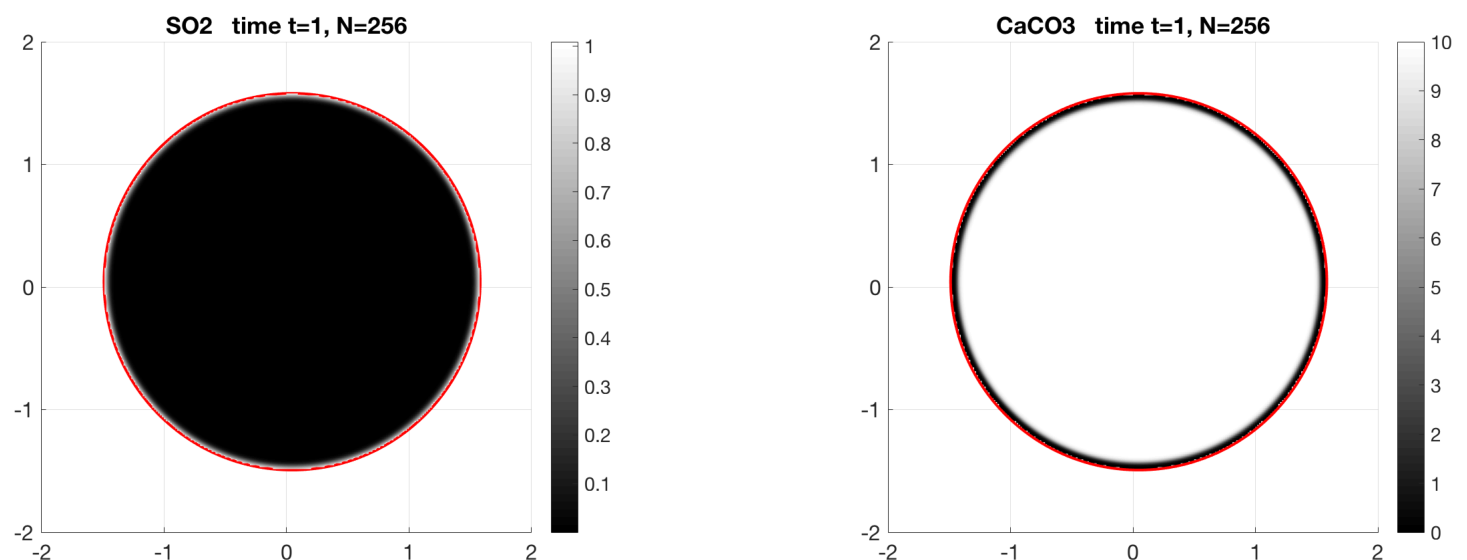
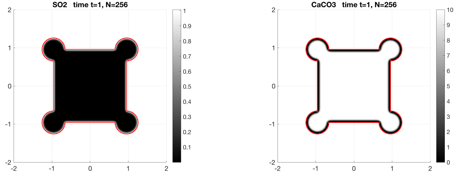
We perform two tests: Test 3 and Test 4, with the domain represented by the level-sets (32) and (33), respectively (see Fig. 7).
Solutions at time are plotted in Figs. 16 and 17. For each W-cycle of the multigrid method, we compute the convergence factor as:
where
is the defect after W-cycles. Convergence factors are plotted in Fig. 18 versus the W-cycle iterations. The first convergence factor obtained in each linear system (11) (either of the same Newton-Raphson step or a new time step) is circled (in red). The convergence factors of the first few linear systems are slightly higher due to the inconsistency of the initial and boundary conditions for . After a few linear systems, the convergence factors are mainly distributed around , which is the predicted value by the Local Fourier Analysis for scalar multigrid in rectangular domains [56, Table 4.1, page 117], showing that the multigrid efficiency has not been degraded by the non-rectangular domain and the ghost-point approach.
4.3 Complex geometries
In this section we show how the method performs on more complex geometries. We use data (31) and (34) and we test three domains: a woman head profile (Test 5), a shark (Test 6) and a necklace (Test 7). The solutions at time are represented in Figs. 19, 21 and 23, respectively, while zooms on some relevant regions, with the contour plot of at times , , and , are represented in Figs. 20, 22 and 24, respectively. In general, we can see that the reaction is quicker around corner points, i.e. regions where the boundary has a higher curvature. For example, in Test 5 the eyelash of the woman is entirely gypsum already at time (top-right plot of Fig. 20), while the hair strands progressively draw back at times , and , and almost disappear at time (top-left plot of Fig. 20). The gypsum formation is also quicker around reentrant corners, as we can see in the bottom-left and bottom-right plots of Fig. 20, for example. Similar conclusions may be drawn for the shark in Test 6, where the teeth (top-right plot of Fig. 22) and the secondary dorsal fin (top-left plot of Fig. 22) are transformed quickly. The damage on the caudal fin is quicker around the tips (top-left plot of Fig. 22) and around the reentrant corner of the pectoral fin (bottom-left plot of Fig. 22) and of the primary dorsal fin (bottom-right plot of Fig. 22). Tests 5 and 6 confirm the qualitative observation made by practitioners in the field of conservation of cultural heritage that the parts of a manufact that are most quickly affected by the sulfation of marble are the higher details of the decoration and the sharp edges. It is important to take into account that gypsum is soluble in water and very prone to breaking due to thermal shocks and thus that the areas with high gypsum content, in a real case, would be quickly lost by dissolution into rainwater or by exfoliation by the dilatation due to the cyclic seasonal temperature variations. Test 7 shows qualitatively analogous results. In fact, the lace connecting the beads is the most quickly damaged part, due to its reduced thickness, followed by the beads in order of size. The larger beads and the diamond shaped pendant are less sulfated and suffer damages almost only close to the reentrant corners. Fig. 23 shows that in this case gypsum dissolution in water or its exfoliation would cause a dramatic topological change, disconnecting the necklace into many separated pieces.


5 Conclusion
Having in mind the modeling of marble degradation under chemical pollutants e.g. the sulfation process, we considered the governing nonlinear equations and their numerical approximation. The space domain is implicitly defined using a level-set approach. We employed a Crank-Nicolson in time, while for the space variables the discretization is performed by a standard Finite-Difference scheme for grid points inside the domain and by a ghost-cell technique on the ghost points (by using boundary conditions).
The solution of the large nonlinear system has been obtained by a Newton-Raphson procedure and by a tailored multigrid technique. All the numerical experiments have given very satisfactory results both from the viewpoint of the reconstruction quality and of the computational efficiency.
As future steps we can include, from the numerical analysis point of view, the spectral analysis of the resulting matrices from a GLT viewpoint [31, 32] having in mind a rigorous convergence analysis of the considered multigrid techniques.
From a modelling point of view, it would be interesting to extend the computational techniques introduced in this paper to the models of degradation processes that employ an evolving domain (e.g. [15]) or that include internal moving interfaces among layers of materials with different properties (e.g. [14, 46]), to take into account some effects like swelling and corrosion. In this respect, we point out that the level-set technique introduced in this paper would be able to track correctly the pristine marble domain even if it was disconnected during the time evolution as in the example of Fig. 23.
From a computational point of view, the method will be extended to three dimensional problems, where a realistic piece of work will be modelled from a laser scanner 3D reconstruction. To reduce the computational cost, the computational strategy will include an Adaptive Meshing Refinement (AMR) approach, where the Cartesian mesh will be refined around critical regions such as the boundary and/or the internal moving interface, by extending AMR strategies already developed for simpler problems [44, 55].
Acknowledgments
The work has been partially supported by the London Mathematical Society Computer Science Small Grants – Scheme 7 (Ref. SC7-1617-02) and the Research in Pairs – Scheme 4 (Ref. 41739).
References
- [1] G. Alì, M. Bisi, G. Spiga, and I. Torcicollo. Kinetic approach to sulphite chemical aggression in porous media. Int. J. Nonlinear Mech., 47(7):769–776, 2012.
- [2] G. Alì, V. Furuholt, R. Natalini, and I. Torcicollo. A mathematical model of sulphite chemical aggression of limestones with high permeability. part i. modeling and qualitative analysis. Transp. Porous Media, 69(1):109–122, 2007.
- [3] P. Angot, C.-H. Bruneau, and P. Fabrie. A penalization method to take into account obstacles in incompressible viscous flows. Numer. Math., 81, 1999.
- [4] D. Aregba Driollet, F. Diele, and R. Natalini. A mathematical model for the aggression to calcium carbonate stones: numerical approximation and asymptotic analysis. SIAM J. Appl. Math., 64(5):1636–1667, 2004.
- [5] T. D. Aslam. A partial differential equation approach to multidimensional extrapolation. Journal of Computational Physics, 193(1):349–355, 2004.
- [6] I. Babuška. The finite element method for elliptic equations with discontinuous coefficients. Computing, 5:207–213, 1970.
- [7] D. Bochkov and F. Gibou. Solving poisson-type equations with robin boundary conditions on piecewise smooth interfaces. Journal of Computational Physics, 376:1156–1198, 2019.
- [8] E. Bonetti, C. Cavaterra, F. Freddi, M. Grasselli, and R. Natalini. A nonlinear model for marble sulphation including surface rugosity: theoretical and numerical results. Comm. Pure Appl. Anal., 18(2):977–998, 2019.
- [9] J. Bramble and J. King. A finite element method for interface problems in domains with smooth boundaries and interfaces. Adv. Comput. Math., 6:109–138, 1996.
- [10] S. Brenner and R. Scott. The mathematical theory of finite element methods, volume 15. Springer Science & Business Media, 2007.
- [11] F. Brezzi and M. Fortin. Mixed and hybrid finite element methods, volume 15. Springer Science & Business Media, 2012.
- [12] F. Chantalat, C.-H. Bruneau, C. Galusinski, and A. Iollo. Level-set, penalization and cartesian meshes: A paradigm for inverse problems and optimal design. Journal of Computational Physics, 228:6291–6315, 2009.
- [13] A. Chertock, A. Coco, A. Kurganov, and G. Russo. A second-order finite-difference method for compressible fluids in domains with moving boundaries. Communications in Computational Physics, 23(1):230–263, 2018.
- [14] F. Clarelli, B. De Filippo, and R. Natalini. Mathematical model of copper corrosion. Applied mathematical modelling, 38(19-20):4804–4816, 2014.
- [15] F. Clarelli, A. Fasano, and R. Natalini. Mathematics and monument conservation: Free boundary models of marble sulfation. SIAM J. Appl. Math., 69(1):149–168, 2008.
- [16] A. Coco, G. Currenti, J. Gottsmann, G. Russo, and C. Del Negro. A hydro-geophysical simulator for fluid and mechanical processes in volcanic areas. Journal of Mathematics in Industry, 6(1):6, 2016.
- [17] A. Coco, G. Currenti, C. D. Negro, and G. Russo. A Second Order Finite-Difference Ghost-Point Method for Elasticity Problems on unbounded domains with applications to Volcanology. Communications in Computational Physics, 16:983–1009, 2014.
- [18] A. Coco and G. Russo. Second order multigrid methods for elliptic problems with discontinuous coefficients on an arbitrary interface, i: one dimensional problems. Numerical Mathematics: Theory, Methods and Applications, 5(1):19–42, 2012.
- [19] A. Coco and G. Russo. Finite-Difference Ghost-Point Multigrid Methods on Cartesian Grids for Elliptic Problems in Arbitrary Domains. Journal of Computational Physics, 241:464–501, 2013.
- [20] A. Coco and G. Russo. Boundary treatment in ghost point finite difference methods for compressible gas dynamics in domain with moving boundaries. In Hyperbolic Problems: Theory, Numerics, Applications, Proceedings to HYP2012, pages 455–465, 2014.
- [21] A. Coco and G. Russo. Second order finite-difference ghost-point multigrid methods for elliptic problems with discontinuous coefficients on an arbitrary interface. Journal of Computational Physics, 361:299–330, 2018.
- [22] F. Di Turo, C. Proietti, A. Screpanti, M. Fornasier, I. Cionni, G. Favero, and A. De Marco. Impacts of air pollution on cultural heritage corrosion at european level: What has been achieved and what are the future scenarios. Environmental Pollution, 218:586–594, 2016.
- [23] J. Dolbow and I. Harari. An efficient finite element method for embedded interface problems. Int. J. for Num. Meth. in Eng., 78(229–252), 2009.
- [24] M. Donatelli, M. Semplice, and S. Serra-Capizzano. Analysis of multigrid preconditioning for implicit PDE solvers for degenerate parabolic equations. SIAM J. Matrix Anal., 32(4):1125–1148, 2011.
- [25] M. Donatelli, M. Semplice, and S. Serra-Capizzano. AMG preconditioning for nonlinear degenerate parabolic equations on nonuniform grids with application to monument degradation. Appl. Numer. Math., 68:1–18, 2013.
- [26] J. Donea. An arbitrary Lagrangian-Eulerian finite element method for transient fluid-structure interactions. Computer Methods in Applied Mechanics and Engineering, 33:689–723, 1982.
- [27] M. Dryja. A neumann-neumann algorithm for mortar discretization of elliptic problems with discontinuous coefficients. Num. Math., 99(645–656), 2005.
- [28] R. E. Ewing, Z. Li, T. Lin, and Y. Lin. The immersed finite volume element methods for the elliptic interface problems. Mathematics and Computers in Simulation, 50(1):63–76, 1999.
- [29] R. Fedkiw, T. Aslam, B. Merriman, and S. Osher. A non-oscillatory Eulerian approach to interfaces in multimaterial flows (the ghost fluid method). Journal of Computational Physics, 152:457–492, 1999.
- [30] L. Formaggia and F. Nobile. Stability analysis of second-order time accurate schemes for ALE-FEM. Computer Methods in Applied Mechanics and Engineering, 193:4097–4116, 2004.
- [31] C. Garoni and S. Serra-Capizzano. Generalized locally Toeplitz sequences: theory and applications. Vol. I. Springer, Cham, New York, 2017.
- [32] C. Garoni and S. Serra-Capizzano. Generalized locally Toeplitz sequences: theory and applications. Vol. II. Springer, Cham, New York, 2018.
- [33] C. Giavarini, M. Santarelli, R. Natalini, and F. Freddi. A non-linear model of sulphation of porous stones: Numerical simulations and preliminary laboratory assessments. J. Cultural Heritage, 9(1):14–22, 2008.
- [34] F. Gibou and R. Fedkiw. A second-order-accurate symmetric discretization of the Poisson equation on irregular domains. Journal of Computational Physics, 176:205–227, 2002.
- [35] F. Gibou and R. Fedkiw. A fourth order accurate discretization for the Laplace and heat equations on arbitary domains, with applications to the Stefan problem. Journal of Computational Physics, 202:577–601, 2005.
- [36] V. Girault and P.-A. Raviart. Finite element methods for Navier-Stokes equations: theory and algorithms, volume 5. Springer Science & Business Media, 2012.
- [37] S. Groí and A. Reusken. An extended pressure finite element space for two-phase incompressible flows with surface tension. Journal of Computational Physics, 224(40–58), 2007.
- [38] A. Hansbo and P. Hansbo. A finite element method for the simulation of strong and weak discontinuities in solid mechanics. Comput. Meth. in Appl. Mech. and Eng., 1993(3523–3540), 2004.
- [39] Á. Helgadóttir, Y. T. Ng, C. Min, and F. Gibou. Imposing mixed dirichlet–neumann–robin boundary conditions in a level-set framework. Computers and Fluids, 121:68–80, 2015.
- [40] C. Hesch and P. Betsch. Isogeometric analysis and domain decomposition methods. Computer Methods in Applied Mechanics and Engineering, 213:104–112, 2012.
- [41] J. Huang and J. Zou. A mortar element method for elliptic problems with discontinuous coefficients. IMA J. Numer. Anal., 22(549–576), 2001.
- [42] D. Lacanette, S. Vincent, A. Sarthou, P. Malaurent, and J.-P. Caltagirone. An eulerian/lagrangian method for the numerical simulation of incompressible convection flows interacting with complex obstacles: Application to the natural convection in the lascaux cave. International Journal of Heat and Mass Transfer, 52(11-12):2528–2542, 2009.
- [43] R. J. LeVeque and Z. Li. The immersed interface method for elliptic equations with discontinuous coefficients and singular sources. Journal of Numerical Analysis, 31:1019–1044, 1994.
- [44] M. Mirzadeh, M. Theillard, and F. Gibou. A second-order discretization of the nonlinear poisson–boltzmann equation over irregular geometries using non-graded adaptive cartesian grids. Journal of Computational Physics, 230(5):2125–2140, 2011.
- [45] Y. T. Ng, C. Min, and F. Gibou. An efficient fluid-solid coupling algorithm for single-phase flows. J. Comput. Phys., 228:8807–8829, 2009.
- [46] C. Nikolopoulos. Mathematical modelling of a mushy region formation during sulphation of calcium carbonate. Netw. Heterog. Media, 9(4):635–654, 2014.
- [47] M. Oevermann, C. Scharfenberg, and R. Klein. A sharp interface finite volume method for elliptic equations on Cartesian grids. Journal of Computational Physics, 228:5184–5206, 2009.
- [48] S. Osher and R. Fedkiw. Level set methods and dynamic implicit surfaces, volume 153. Springer Science & Business Media, 2006.
- [49] S. Osher and J. A. Sethian. Fronts propagating with curvature-dependent speed: algorithms based on hamilton-jacobi formulations. Journal of computational physics, 79(1):12–49, 1988.
- [50] C. S. Peskin. Numerical analysis of blood flow in the heart. Journal of Computational Physics, 25:220–252, 1977.
- [51] M. Saba, E. Quiñones-Bolaños, and A. Barbosa López. A review of the mathematical models used for simulation of calcareous stone deterioration in historical buildings. Atmospheric Environment, 180:156–166, 2018.
- [52] M. Semplice. Preconditioned implicit solvers for nonlinear PDEs in monument conservation. SIAM J. Sci. Comput., 32(5):3071–3091, 2010.
- [53] J. Seo, S.-y. Ha, and C. Min. Convergence analysis in the maximum norm of the numerical gradient of the shortley–weller method. Journal of Scientific Computing, 74(2):631–639, 2018.
- [54] G. H. Shortley and R. Weller. The numerical solution of Laplace’s equation. J. Appl. Phys., 9:334–348, 1938.
- [55] M. Theillard, C. H. Rycroft, and F. Gibou. A multigrid method on non-graded adaptive octree and quadtree cartesian grids. Journal of Scientific Computing, 55(1):1–15, 2013.
- [56] U.Trottemberg, C. Oosterlee, and A. Schuller. Multigrid. Academic Press, 2000.
- [57] G. Xu, B. Mourrain, R. Duvigneau, and A. Galligo. Parameterization of computational domain in isogeometric analysis: methods and comparison. Computer Methods in Applied Mechanics and Engineering, 200(23-24):2021–2031, 2011.
- [58] S. Yu, Y. Zhou, and G. Wei. Matched Interface and Boundary (MIB) method for elliptic problems with sharp-edged interfaces. Journal of Computational Physics, 224:729–756, 2007.