First Identification of 10- [C ii] Halos
around Star-Forming Galaxies at
Note: ApJ in press
Abstract
We report the discovery of 10-kpc [Cii] 158m halos surrounding star-forming galaxies in the early Universe. We choose deep ALMA data of 18 galaxies each with a star-formation rate of with no signature of AGN whose [Cii] lines are individually detected at , and conduct stacking of the [Cii] lines and dust-continuum in the -visibility plane. The radial profiles of the surface brightnesses show a 10-kpc scale [Cii] halo at the 9.2 level, significantly more extended than the HST stellar continuum data by a factor of on the exponential-profile basis, as well as the dust continuum. We compare the radial profiles of [Cii] and Ly halos universally found in star-forming galaxies at this epoch, and find that the scale lengths agree within level. While two independent hydrodynamical zoom-in simulations match the dust and stellar continuum properties, the simulations cannot reproduce the extended [C ii] line emission. The existence of the extended [Cii] halo is the evidence of outflow remnants in the early galaxies and suggest that the outflows may be dominated by cold-mode outflows expelling the neutral gas.
Subject headings
galaxies: formation — galaxies: evolution — galaxies: high-redshiftI. Introduction
Galaxy size and morphological studies in the early Universe provide important insights into the initial stage of galaxy formation and evolution. The size and morphology in the rest-frame ultra-violet (UV) and far-infrared (FIR) wavelengths trace the areas of young star formation and the active starbursts that are less and heavily obscured by dust, respectively. The [Cii] fine-structure transition at 1900.5469 GHz (157.74 m) is a dominant coolant of the inter-stellar medium (ISM) in galaxies (Stacey et al. 1991; De Looze et al. 2014, e.g.,), whose size and morphology are strong probes of ISM properties. Comparing the size and morphology in the rest-frame UV+FIR continuum and the [Cii] 158-m line is thus important to comprehensively understand the evolutionary process via the star-formation surrounded by the ISM.
The Hubble Space Telescope (HST) has revealed the size and morphological properties in the rest-frame UV wavelengths for the high-redshift galaxies up to (Oesch et al. 2010; Ono et al. 2013; Shibuya et al. 2015; Bouwens et al. 2017; Kawamata et al. 2018, e.g.,). These HST studies show that star-forming galaxies generally have an exponential-disk profile and become compact toward high redshifts.
The Atacama Large Millimeter / submillimeter Array (ALMA) has opened our views to the obscured star-formation and the [Cii] line properties in the rest-frame FIR wavelength up to (Watson et al. 2015; Maiolino et al. 2015; Capak et al. 2015; Pentericci et al. 2016; Knudsen et al. 2016; Matthee et al. 2017; Carniani et al. 2018; Smit et al. 2018; Hashimoto et al. 2018, e.g.,). There have also been several attempts to measure the size and morphology in the rest-frame FIR continuum and the [Cii] line for such high redshift galaxies at 57, where Carniani et al. 2017 report that the effective radius of the [Cii] line-emitting region is larger than that of the rest-frame UV region. However, large uncertainties still remain due to the small number statistics and observational challenges.
One critical challenge is sensitivity. The recent ALMA studies show that signal-to-noise ratio (S/N) 10 is needed to obtain reliable size measurement results both on the image-based and visibility-based analyses (Simpson et al. 2015; Ikarashi et al. 2015, e.g.,), while the majority of the previous ALMA detections of the dust continuum and the [Cii] line from 57 galaxies show the S/N less than 10. If the S/N level is poor, noise fluctuations significantly affect the profile fitting results. Moreover, Hodge et al. 2016 show that the combination of the original smoothed galaxy profile and the noise fluctuations can make the morphology more clumpy. To obtain the reliable size and morphological results, extensively deep observations are thus required.
In this paper, we determine the size and morphology for the dust continuum and the [Cii] line in the star-forming galaxies at via the stacking technique in the -visibility plane, utilizing new and archival deep ALMA Band 6/7 data. In conjunction with deep HST images, we study the general morphology of the total star-formation and the ISM in the epoch of re-ionization. The structure of this paper is as follows. In Section 2, the observations and the data reduction are described. Section 3 outlines the method of [Cii] line detections, line velocity width, source position measurements, and the stacking processes of ALMA and HST data. We report the results of the radial profiles of the [Cii] line, rest-frame FIR, and rest-frame UV wavelengths in Section 4. In Section 5, we discuss the physical origin of the extended [Cii] line emission, comparing with the zoom-in cosmological simulation results. A summary of this study is presented in Section 6.
| Target | R.A | Dec. | () | EWLyα | † | Beam | ALMA ID | HST | Ref. | |
| (J2000) | (J2000) | (mag) | () | (Jy/beam) | () | |||||
| (1) | (2) | (3) | (4) | (5) | (6) | (7) | (8) | |||
| Literature | ||||||||||
| WMH5 | 36.612542 | 4.877333 | 6.069 (6.076) | 22.6 | 13.0 | 8 | 0.500.46 | 2013.1.00815.S | N | W15, J17 |
| 2015.1.00834.S | W15, J17 | |||||||||
| CLM1 | 37.012319 | 4.271706 | 6.166 (6.176) | 22.6 | 50.0 | 18 | 0.520.45 | 2013.1.00815.S | N | W15 |
| COS301855 | 150.125803 | 2.266613 | 6.854 (-) | 21.9 | 2.9 | 27 | 1.080.74 | 2015.1.01111.S | Y | S18 (S15) |
| COS298703 | 150.124400 | 2.217294 | 6.808 (6.816) | 22.0 | 16.2 | 25 | 1.070.74 | 2015.1.01111.S | Y | S18 (S15) |
| NTTDF6345 | 181.403878 | 7.756192 | 6.698 (6.701) | 21.5 | 15.0 | 20 | 1.250.97 | 2015.1.01105.S | N | P16 |
| BDF2203 | 336.958267 | 35.147529 | 6.122 (6.118) | 20.9 | 9.9 | 20 | 1.851.05 | 2016.1.01240.S | N†† | C18 |
| COS13679 | 150.099014 | 2.343517 | 7.142 (7.145) | 21.4 | 15.0 | 18 | 0.850.85 | 2015.1.01105.S | N‡ | P16 |
| COS24108 | 150.197356 | 2.478931 | 6.623 (6.629) | 21.6 | 27.0 | 20 | 0.810.75 | 2015.1.01105.S | N‡ | P16 |
| Hz1 | 149.971828 | 2.118142 | 5.689 (5.690) | 22.0 | 5.3 | 27 | 0.750.52 | 2012.1.00523.S | Y | C15 (B17) |
| Hz2 | 150.517186 | 1.928936 | 5.670 (5.670) | 21.9 | 6.9 | 35 | 0.830.53 | 2012.1.00523.S | N‡ | C15 (B17) |
| Hz3 | 150.039247 | 2.3371611 | 5.542 (5.546) | 21.7 | 3.6 | 47 | 0.770.42 | 2012.1.00523.S | Y | C15 (B17) |
| Hz4 | 149.618760 | 2.051850 | 5.544 (5.310) | 22.3 | 10.2 | 64 | 0.890.51 | 2012.1.00523.S | Y | C15 (B17) |
| Hz6 | 150.089576 | 2.586324 | 5.293 (5.290) | 22.8 | 8.0 | 32 | 0.670.50 | 2012.1.00523.S | Y | C15 (B17) |
| Hz7 | 149.876925 | 2.134061 | 5.253 (5.250) | 21.8 | 9.8 | 35 | 0.470.38 | 2012.1.00523.S | Y | C15 (B17) |
| Hz8 | 150.016894 | 2.626631 | 5.153 (5.148) | 21.8 | 27.1 | 30 | 0.400.29 | 2012.1.00523.S | Y | C15 (B17) |
| Hz9 | 149.965404 | 2.378358 | 5.541 (5.548) | 21.9 | 14.4 | 43 | 0.640.54 | 2012.1.00523.S | Y | C15 (B17) |
| New Detection | ||||||||||
| NB816S61269 | 34.438567 | 5.493392 | 5.684 (5.688) | 20.4 | 93.3 | 22 | 0.450.42 | 2012.1.00602.S | N | F16 |
| WMH13 | 149.985580 | 2.207528 | 5.985 (5.983) | 22.0 | 27.0 | 16 | 1.150.89 | 2013.1.00815.S | N | W15 |
Notes:
(1) Spectroscopic redshift determined by the [Cii] (Ly) line emission.
(2) Absolute magnitudes.
(3) Rest-frame Ly EW.
(4) One sigma noise measured by the standard deviation of the pixel values in the continuum map before primary beam correction.
(5) Synthesized beam size of our ALMA maps (weighting = ”natural”).
(6) ALMA project ID.
(7) ”Y” (”N”) indicates the sources (not) included in the ALMA-HST sample. (8) ALMA (HST) data reference (W15: Willott et al. 2015, J17: Jones et al. 2017, S18: Smit et al. 2018, P16: Pentericci et al. 2016, C18: Carniani et al. 2018, S15: Smit et al. 2015, C15: Capak et al. 2015, B17: Barisic et al. 2017, F16: Fujimoto et al. 2016).
Our additional flagging and difference in the imaging parameter setting may produce different values from the data references.
Although there is the F105W data, we do not include this source in the ALMA-HST sample due to the differences in the PSF and the rest-frame wavelength from the F160W data.
Although there is the F160W data, we do not include these sources in the ALMA-HST sample due to the large offsets even after the astrometry correction (see text).
Throughout this paper, we assume a flat universe with , , , and km s-1 Mpc-1. We use magnitudes in the AB system (Oke & Gunn 1983).
II. Sample and Data Reduction
II.1. Our ALMA Sample
The sample is drawn mainly from the literature (Capak et al. 2015; Willott et al. 2015; Pentericci et al. 2016; Smit et al. 2018; Carniani et al. 2018; Jones et al. 2017), selecting only star-forming galaxies at whose [C ii] lines have been detected (at signal-to-noise, S/N 5) with ALMA. To obtain reliable results for representative galaxies in the early Universe, we limit our sample to galaxies with (i) star-formation rates (SFRs), M⊙ yr-1, (ii) no indication of AGN activity, (iii) no giant Ly systems, such as Himiko (Ouchi et al. 2009) and CR7 (Matthee et al. 2015), (iv) no signs of gravitationally lensing, e.g. galaxies behind massive galaxy clusters, (v) [C ii] line emission with a full width at half maximum (FWHM) broader than 80 km s-1, and (vi) [C ii] line detections that are reproduced in our own data reduction. We adopt (v) because the thermal noise fluctuation can produce peaky false source signals even with S/N 5, when we examine the large volume data such as the ALMA 3D data cubes. Note that our sample does not include the tentative [C ii] line detections reported in the ALMA blind line survey (Aravena et al. 2016; Hayatsu et al. 2017), because these tentative [C ii] detections have not been spectroscopically confirmed. We identify 16 [C ii] line sources that meet the above criteria in the literature. Table 1 summarises our sample and the references that describe the relevant ALMA observations.
In addition to the literature sample, we include new [C ii] line detections of two star-forming galaxies, NB816-S-61269 (Ouchi et al. 2008; Fujimoto et al. 2016) and WMH13 (Willott et al. 2013a) at and , respectively. In Figure 1, we present the velocity-integrated maps and the spectra for these two [C ii] detections. In the velocity-integrated maps of NB816-S-61269 and WMH13, the [C ii] line is detected with peak S/N levels of 5.6 and 5.2, respectively; rest-frame FIR dust continuum emission is not detected from either galaxy. The details of the ALMA observations for these additional sources are listed in Table 1.

From the literature and the additional samples, we obtain a total of 18 [Cii] line sources. The 18 [Cii] line sources have the spectroscopic redshifts determined by the [Cii] lines () and the absolute rest-frame UV magnitudes () in the ranges of and 22.8 to 20.4 (SFR /yr). We summarize the physical properties of , , and the Ly equivalent-width (EWLyα) in Table 1.
II.2. ALMA Data
We reduce the ALMA data for our sample with the Common Astronomy Software Applications package (CASA; McMullin et al. 2007) in the standard manner with the scripts provided by the ALMA observatory. In this process, we carry out re-calibrations for the flux density and additional flagging for bad antennae if we find problems in the final images that shows striped patterns and/or significantly higher noise levels than expected. The continuum images and line cubes are produced by the CLEAN algorithm with the tclean task with a pixel scale of . For the line cubes, the velocity channel width is re-binned to 20 km s-1, where the velocity center is adjusted to the Ly redshift. We do not CLEAN the line cubes because the [Cii] line is faint in each 20-km s-1 channel. The CLEAN boxes were set at the peak pixel positions with S/N 5 in the auto mode, and the CLEAN routines were proceeded down to the 3 level. We list the standard deviation of the pixel values in a final natural-weighted image and a synthesized beam size for the continuum image in Table 1.
Note that the continuum is subtracted from the -data of the line cubes for 4 sources (Hz4, Hz6, Hz9, and WMH5) whose continuum emission is individually detected (Capak et al. 2015; Willott et al. 2015). The continuum level is estimated from the channels in the velocity range of 2 FWHM in the same baseband as the [C ii] line emission.
II.3. HST Data
To study the rest-frame UV properties of our sample, we also use the HST Wide Field Camera 3 (WFC3) in F160W, 1.54 m (-band), images from the Hubble Legacy Archive, where we obtain final flat-field and flux-calibrated science products.
To correct the potential offsets of the HST astrometry (Rujopakarn et al. 2016; Dunlop et al. 2017, e.g.,), we calibrate the astrometry of the -band maps with the Gaia Data Release 2 catalog (Gaia Collaboration et al. 2018). First, we identify bright objects in the -band images with sextractor version 2.5.0 (Bertin & Arnouts 1996). Second, we cross-match the bright -band objects and the GAIA catalog. Finally, we evaluate offsets between the bright -band object centers and the GAIA catalog positions. We find that the bright -band object centers indeed have the offsets from the GAIA catalog in the range of . We correct the astrometry of each -band map to match the GAIA catalog based on these offsets. With the above procedure, the majority of our sample shows that the [C ii] line and the -band continuum have a consistent peak position within the offset smaller than . However, the large offset over still remains in some cases, probably because the astrometry correction does not work successfully, or we witness the intrinsic offset between the [C ii] line and the rest-frame UV continuum (Maiolino et al. 2015, e.g.,). In any cases, these objects with the large offsets cause the smearing effect in the stacking results. To securely study the morphological property from the stacking results, we do not include these objects in the following HST data analyses. We identify that 9 out of 18 sources in our sample have been observed with the HST/-band whose astrometry is successfully corrected. We refer to the 9 and the 18 sources as the ”ALMA-HST” and ”ALMA-ALL” samples, respectively. In Table 1, we summarize the HST data references and the sources included in the ALMA-HST sample.
Note that we confirm that the ALMA astrometry is well consistent with the GAIA catalog within a milli-arcsec scale via the bright quasars used as the phase calibrators in the ALMA observations. Thus, we do not carry out any astrometry corrections for our ALMA maps.
III. Data Analysis


III.1. 3D Position in ALMA Cube
To carry out stacking for the [C ii] line and the rest-frame FIR continuum, we estimate source centroids for the 18 [C ii] line sources in the ALMA 3-dimensional data cubes via the following six steps: (1) We create fiducial [C ii] velocity-integrated maps in the velocity range, 100–900 km s-1, that maximizes the S/N level of the [C ii] line detection. (2) We measure fiducial positional centroids based on the peak pixel positions (pixel scale = ) in the fiducial [C ii] velocity-integrated maps, having smoothed spatially with a -taper of . (3) We produce [C ii] spectra with an aperture diameter of at the fiducial source centroids. (4) We obtain the peak frequencies and FWHMs of the [C ii] line emission by fitting a single Gaussian to the [C ii] spectra. (5) We re-create velocity-integrated maps with velocity ranges of the FWHM. (6) We measure final positional centroids in the new velocity-integrated map in the same manner as step (2). Note that we use the smoothed map (via the -taper) instead of the naturally-weighted map in steps (2) and (6) because Monte-Carlo simulations in the -visibility plane show that smoothed maps have lower uncertainties in the positional measurements than the intrinsic maps (Fujimoto et al. 2018). We list the final positional centroids and redshifts in Table 1.
III.2. ALMA Visibility-based Stacking
We carry out visibility-based stacking for our ALMA data via the following procedure. First, we split the visibility data into the [C ii] line and the rest-frame FIR continuum datasets. For the [C ii] line dataset, we extract the visibility data with the [C ii] line channels across a velocity range of 100 km s-1 (= 50 km s-1), where the velocity center is the [C ii] frequency peak (the 3D position in our ALMA cubes). We do not adopt a wider velocity range because of the potential contamination of the close companions (Jones et al. 2017; Carniani et al. 2018). For the rest-frame FIR continuum dataset, we produce the visibility data whose [C ii] line channels in a velocity range of 2FWHM are fully removed. Second, we shift the coordinate of the visibility datasets by re-writing the source center determined in Section III.1 as ”00:00:00.00 00:00:00.0” with stacker (Lindroos et al. 2015). Third, we combine the visibility datasets with the concat task. Fourth, we re-calculate the data weights for the combined visibility datasets with the statwt task, based on the scatter of visibilities, which includes the effects of integration time, channel width and system temperature. Finally, we obtain the stacked datasets of the [C ii] line and the rest-frame FIR continuum. The central frequency in the [C ii] line dataset is 271.167 GHz which corresponds to the [C ii] redshift at . Assuming the redshift of as the weighted average source redshift of our sample, we adopt the angular scale of kpc in the following analyses. Note that we adopt the -band peak positions (Section III.3) as the common stacking center for the ALMA-HST sample.
Figure 2 indicates the -visibility coverage after the visibility-based stacking for the ALMA datasets of the ALMA-ALL sample. For comparison, the -visibility coverage for an individual dataset, before stacking, is also plotted. In the stacked data, the -visibility coverage is well sampled, especially for the short baselines, k, which is important to recover the flux density from diffuse, extended structures.
In Figure 3, we show the natural-weighted images of the [Cii] line and dust continuum after the visibility-based stacking for the ALMA-ALL (ALMA-HST) sample, where the standard deviation of the pixel values in the dust continuum image achieves 4.1 (8.3) Jy/beam with the synthesized beam size of (). The peak pixel signal-to-noise (S/N) ratio shows 21 (20) and 10 (8) significance levels for the [Cii] line and dust continuum, respectively, for the ALMA-ALL (ALMA-HST) sample. The spatially resolved [C ii] line emission in the ALMA-ALL sample is detected at the 9.3 level in the aperture radius of 10 kpc even after masking the emission in a central area up to 2FWHM of the ALMA synthesized beam, based on the random-aperture method. Because the extended structure is difficult to be modeled by the clean algorithm perfectly, we use the dirty images for both the [C ii] line and the rest-frame FIR continuum in the following analyses.

In Figure 4, we present the radial surface brightness profile of the stacked [C ii] line, and summarize various tests for the extended [C ii] line structure. First, we compare our stacking and individual results. In the top left panel of Figure 4, we show the individual results for several [C ii] line sources whose lines are detected at high S/N, with an ALMA beam size of to recover the diffuse, extended structures. We find that the stacked results are consistent with the individual results within the scatter, suggesting that our ALMA stacking result provides a faithful representative of the 18 [C ii] line sources. Second, we evaluate the uncertainty of the sample variance. We make 18 newly stacked data with 17 [C ii] line sources, i.e., in each newly stacked data we remove one source from the full sample, and derive the 18 [C ii] radial profiles. In the top right panel of Figure 4, the red shaded area indicates the 16–84 percentiles of these 18 radial profiles. The [C ii] radial profile is extended up to the radius of 10 kpc even including the sample variance, suggesting that the sample variance does not change our results of the existence of the extended [C ii] line emission. Third, we investigate whether the extended [C ii] line structure is caused by any specific data properties. We remove the sources that are I) taken with the lowest resolutions (BDF2203, NTTDF6345, and WMH13), and II) reported to have companions (WMH5, Hz2, Hz6, and Hz8; Jones et al. 2017; Carniani et al. 2018), and obtain newly stacked data. In the top right panel of Figure 4, we present the radial profiles of the [C ii] line emission in the newly stacked data. We find that the newly stacked [C ii] line profiles reproduce the extended structures that are well consistent with the original stacking result in the ALMA-ALL sample. This indicates that the extended [C ii] line structure is not caused either by the bias to the low-resolution data or the contamination of the companions. Fourth, we examine the surface brightness dimming effect among our sample. We divide the 18 [C ii] line sources into two subsamples: low () and high-redshift () samples, and obtain other newly stacked data. In the bottom left panel of Figure 4, we show the radial profiles of the [C ii] line emission in both subsamples. We find that the [C ii] line profiles in both subsamples reproduce the extended structures that have good agreements with the original stacking result in the ALMA-ALL sample. This suggests that the surface brightness dimming effect does not significantly affect our stacking results. Fifth, we compare the structures of the [C ii] line and the dust continuum in the same significance level. We produce a random noise map smoothed by the ALMA beam, and combine the noise and the stacked [C ii] line maps. Changing the noise levels, we obtain the noise-enhanced [C ii] line map whose peak S/N ratio becomes comparable to the dust continuum one. We create the 50 noise-enhanced [C ii] line maps. In the bottom right panel of Figure 4, we show the 16–84th percentile of the [C ii] radial profile in the noise-enhanced maps. We find that the [C ii] line profile still exceeds more than the dust continuum in these noise-enhanced maps, showing that the different structures between the [C ii] line and the dust continuum are not mimicked by the difference in the dynamic range.
III.3. HST/H-band Stacking
We have performed image-based stacking for the ALMA-HST sample, exploiting their deep archival HST -band imaging. Before stacking, we carry out the following procedure: 1) We cut out stamps from the -band images, around the [C ii] line sources, and set the pixel scale to , which corresponds to our ALMA images. 2) We identify low-redshift contaminants within from the [C ii] sources, by cross-matching the [C ii] line source positions with photometric redshift catalogs (Ilbert et al. 2013; Skelton et al. 2014). 3) We remove the low-redshift contaminants from the -band images by fitting Srsic profiles (Sérsic 1963) with galfit (Peng et al. 2010). We then proceed to generate an average stack, weighted by the noise levels of the ALMA images of the [C ii] line source. This is because the visibility-based stacking for our ALMA data is weighted by the visibility scatter, which generally corresponded to the noise levels on the ALMA images.
In panel (f) of Figure 5, we show the stacked -band image for the ALMA-HST sample. In the HST stacking, we adopted stacking centroids defined by the peak positions of the -band images, smoothed with the -tapered ALMA beams in a consistent manner with the [C ii] line stacking.
To directly compare the size and morphology of the HST and ALMA images, we need to convolve the HST image to obtain a PSF that resembles the one of the ALMA image. We use galfit to obtain a kernel with which the -band PSF can be converted to the ALMA beam. For the kernel, we assume a sum of three independent Srsic profiles whose positions are fixed at the center.
In Figure 5, we present a schematic overview of converting the -band PSF to the ALMA beam with the best-fit kernel. We first convolve the HST PSF (panel a) with the best-fit kernel (panel b) and derive the mock ALMA beam (panel c). We then subtract the actual ALMA beam (panel d) from the mock ALMA beam and produce the residual map (panel e). Within a radius of on the residual map, we find that the difference between the mock and actual ALMA beams are less than %, showing that the best-fit kernel reproduces the ALMA beams well from the -band PSF. We finally apply the convolution to the stacked -band image (panel f) with the best-fit kernel, and obtain the mock -band image whose PSF is almost the same as the stacked ALMA image.

IV. Results
IV.1. Discovery of [Cii] Halo

Figure 6 presents the radial surface brightness profiles of the [Cii] line, rest-frame FIR, and UV continuum, derived from the stacking results for the ALMA-HST (circles) and ALMA-ALL (squares) samples. For a fair comparison, the ALMA-HST results are obtained by re-performing the ALMA visibility-based stacking with the HST/-band peak positions, while the ALMA-ALL results are not due to the lack of the HST/-band images.
In Figure 6, the ALMA-ALL and ALMA-HST results show a good agreement in both profiles of the [C ii] line and the rest-FIR continuum. We find that the radial profile of the [C ii] line emission is extended up to a radius of 10 kpc which contrasts the rest-frame UV and FIR continuum. Because the typical effective radius of the normal star-forming galaxies at is estimated to be less than 1 kpc (Shibuya et al. 2015, e.g.,), the 10-kpc scale structure at this epoch corresponds to the circum-galactic medium (CGM) surrounding the galaxies. These results suggest that the [Cii] line emission is produced in the wide CGM areas even without stellar continuum. We discuss the physical origin of the [Cii] halo in Section V.
We also find that the profiles of the rest-frame FIR and UV continuum are consistent within the 1 errors. Note that the rest-frame FIR continuum is likely to follow the ALMA beam, while the rest-frame UV continuum is slightly resolved with the ALMA beam. This suggests that the intrinsic size of the rest-frame FIR continuum is smaller than that of the rest-frame UV continuum, which is consistent with the recent ALMA results of the compact rest-frame FIR size more than the rest-frame UV and optical sizes among the star-forming galaxies at (Simpson et al. 2015; Ikarashi et al. 2015; Hodge et al. 2016; Fujimoto et al. 2017; Fujimoto et al. 2018, e.g.,).
IV.2. Effect of [C ii]-UV offset
Recent studies report a possibility that [Cii]-line emitting regions are physically offset from the rest-frame UV ones (Maiolino et al. 2015, e.g.,). To evaluate the potential effect from the [Cii]-UV offsets in our results, we perform the ALMA and HST stacking for the ALMA-HST sample by adopting two different stacking centers: HST/-band and ALMA [C ii] line peak positions, and compare the radial profiles from these stacking results.
In Figure 7, the circle and cross symbols represent the stacking results derived with the common stacking centers of the HST/-band continuum and ALMA [C ii] line peak positions, respectively. We find that the [C ii] line profile is extended more than both the rest-frame FIR and UV continuum profiles in any cases. This suggests that the [C ii] line originates from much wider regions than the continuum emission at rest-frame FIR and UV wavelengths, and clearly shows that the extended structure of the [C ii] line is not caused by the [Cii]–UV offsets.

IV.3. Radial ratio of to total SFR
To test whether the extended [C ii] line structure is caused by satellite galaxies, we investigate radial values of the [C ii] line luminosity at a given SFR derived from the rest-frame FIR and UV continuum. Because the ALMA-ALL and ALMA-HST results are consistent with each other (Figure 6), we adopt the rest-frame UV results from the ALMA-HST sample, while the [C ii] line and rest-frame FIR continuum results from the ALMA-ALL sample to reduce the errors in the following estimates.

We first estimate the radial value. For our sources, the weighted-average source redshift and FWHM of the [C ii] line width are estimated to be and 270 km s-1, respectively. Since the velocity-integrated width is 100 km s-1 in the stacked [C ii] line map, we correct the velocity-integrated value in the range from 100 km s-1 to 270 km s-1, assuming a single Gaussian line profile, to recover the total value of . We second evaluate the radial SFR value. We derive the obscured (SFRIR), un-obscured (SFRUV), and total SFR (SFRtotal) with the equations in Murphy et al. 2011 of
| (1) | |||||
| (2) | |||||
| (3) |
where is the integrated IR flux density estimated by a typical modified blackbody whose spectral index and dust temperature are (Planck Collaboration et al. 2011) and K (Coppin et al. 2008), and is the rest-frame UV luminosity at 0.16 m with the HST -band. Finally, we divide the radial values by the radial SFR values and obtain the radial ratio of /SFRtotal.
In Figure 8, we show the surface densities of () and SFRtotal () as a function of radius (middle panel), and the radial ratio of /SFRtotal (right panel) as a function of SFRtotal for our stacking results. For comparison, the right panel of Figure 8 also presents global scale /SFRtotal ratios of the local dwarf galaxies (De Looze et al. 2014).
In the right panel of Figure 8, the red filled and open circles denote our stacking results in the outer (radius of 4 kpc) and central ( 4 kpc) regions, respectively. We find that /SFRtotal decreases with SFRtotal. The highest ratios () are found at the outer regions and not compatible with typical values found in the local dwarf galaxies (; black dots in the figure). These results indicate that the [C ii] halo is not likely driven by satellite galaxies. Note that other types of high- galaxies with SFRtotal 10 such as star-forming, submillimeter, and quasar-host galaxies show ratios of 10 (Capak et al. 2015; Rybak et al. 2019; Venemans et al. 2019, e.g.,) which are yet difficult to explain the highest ratios in our stacking results ().
Díaz-Santos et al. 2014 report the [C ii] line emission extended over kpc scale around local luminous infrared galaxies (LIRGs), and we also compare our results with this spatially resolved data. In the right panel of Figure 8, we show the /SFRtotal ratios of the extended emission around local LIRGs. We find that the highest ratios in our stacking results () are still higher than those around the local LIRGs (; green crosses in the figure). The [C ii] halo at is thus not identical to the extended [C ii] line emission observed in the local Universe, which may suggest that [C ii] halos evolve with redshift. We discuss possible origins of the [C ii] halo in Section V.
IV.4. Scale Length of [Cii] Halo
We characterize the detail radial surface brightness profile of the [Cii] line emission by two-component fitting with galfit. Here we assume the two components as the central and the halo components.
For the central component, we adopt the Srsic profile whose parameters are estimated from the rest-frame UV profile in the stacked HST/-band image (Figure 5 f). We obtain the best-fit effective radius and the Srsic index of kpc and that are consistent with the average values estimated from the normal star-forming galaxies at (Shibuya et al. 2015). For the halo component, we utilize the exponential profile. The exponential profile has been used for scale-length measurements of the Ly halo which is universally identified around the high-z star-forming galaxies (Steidel et al. 2011; Matsuda et al. 2012; Momose et al. 2014; Momose et al. 2016; Leclercq et al. 2017, e.g.,). The exponential profile is described as exp() where is a constant and is the scale length. We fix the central positions of both central and halo components to obtain a stable result.
Top panel of Figure 9 presents the best-fit results with the Srsic+exponential profiles for the [Cii] line emission. We obtain the best-fit scale-length values of 3.3 0.1 kpc. This corresponds to the best-fit effective radius of 0.1 kpc, showing that the [C ii] halo is extended 5 times more than the stellar continuum in the central galactic component. Note that the visibility-based profile fitting with uvmultifit (Martí-Vidal et al. 2014) also provides us with the best-fit value of 1.7 kpc for the halo component, which is consistent with the galfit result within the error.

In Figure 9, we compare the radial surface brightness profiles of the [Cii] with the Ly halos universally identified in the normal star-forming galaxies at –6 (Momose et al. 2016; Leclercq et al. 2017, e.g.,). For the [Cii] line emission, we adopt the result from the ALMA-ALL sample due to the high significance detection. For the Ly line emission, we use the recent results with the deep MUSE data for the high- LAEs of Leclercq et al. 2017, where the authors estimate the best-fit radial surface brightness profiles by fitting the two-component Srsic+exponential profile. We select the best-fit results of 6 LAEs at with mag and EWLyα 100 that are consistent with the parameter space of our sample (Table 1). We find that the radial surface brightness profile of the [Cii] line emission is comparable to that of the Ly line emission. The median value for the 6 LAEs is estimated to be kpc that is consistent with our best estimate of kpc. These results may imply that the physical origin of the extended [Cii] line emission is related to the Ly halo.
Note that we confirm that it is hard to reproduce the extended morphology of the [C ii] line emission with the central component alone. In the bottom panel of Figure 9, we present the residuals of the [C ii] line emission obtained from the best-fit results of the one- (central) and two- (central+halo) component fittings with uvmultifit. We find that the residuals in the one-component fitting result show a bump at a radius of over the errors, while the residuals in the two-component fitting result is broadly consistent with zero. This suggests that the extended morphology of the [C ii] line emission consists of a combination of the central plus halo components.
IV.5. [C ii] Stacked Spectrum
We also perform the stacking for the [C ii]-line spectra of the ALMA-ALL sample to test whether our ALMA sample has a broad wing feature which is a good probe for the on-going outflow activities. For the stacking procedure, we adopt the same manner as previous ALMA studies (Decarli et al. 2018; Bischetti et al. 2018). Here we adopt a relatively small aperture diameter of for the individual spectra to reduce the contamination of the close companions (Jones et al. 2017; Carniani et al. 2018).
In Figure 10, we show the stacked [C ii]-line spectrum with the best-fit two Gaussian component model: the combination of the core and broad components whose velocity centers are fixed at 0 km/s for the stable results. The best-fit FWHMs are estimated to be 296 40 km/s and 799 654 km/s for the core and broad components, respectively. In the velocity range of 400 – 800 km/s, the velocity-integrated intensity is tentatively detected at the 3.2 level. Moreover, Sugahara et al. 2019 have recently reported that the rest-frame UV metal absorption lines are blue-shifted with the central outflow velocity of 440 km s-1 from the [C ii]-systemic redshift in the stacked Keck spectra whose stacking sample includes 6 out of our 18 [C ii] line sources. These results may suggest the existence of the tentative broad wing feature is produced by the outflow.
Note that there are other possibilities that produce the broad wing feature. One possibility is that the contamination of the satellite galaxies. The [C ii] line emission from the individual satellite galaxies can be smoothed in the stacking procedure for the 18 galaxies, which may be identified as the broad wing feature. Another possibility is that the faint continuum emission is mistakenly identified as the broad wing feature. Although we have performed the continuum subtraction for the [C ii] line data cubes of the 4 galaxies whose continuum emission is individually detected, it is possible that the faint continuum emission from the rest of the 14 ( 18 4) galaxies appears in the deeply stacked spectrum. Since the significance of the broad wing is low, we cannot draw definite conclusions from our data.

IV.6. Comparison with Model
We compare our observational results with two independent numerical simulations for star-forming galaxies with the halo mass of M⊙ at . Note that our sample is characterized by the average value of mag (Table 1) which corresponds to from the – relation (Harikane et al. 2018).
First set is a zoom-in simulation for a star-forming galaxy, Altha (Pallottini et al. 2017a; Pallottini et al. 2017b; Behrens et al. 2018). The hydrodynamical and dust radiative transfer (RT) simulations are combined, which provides realistic predictions for the spatial distribution of the [C ii] line as well as the rest-frame FIR and UV continuum emission, with a spatial resolution of 30 pc. The hydrodynamical and the dust RT simulations are fully described in previous studies (Pallottini et al. 2017a; Pallottini et al. 2017b; Behrens et al. 2018). Note that the dust RT is calculated as a post-processing step on snapshots of the hydrodynamical simulation. The [C ii] line emission is computed in post-processing (Vallini et al. 2015) by adopting the photoionization code, cloudy (Ferland et al. 2017). In these processes, CMB suppression (da Cunha et al. 2013; Zhang et al. 2016; Pallottini et al. 2015; Lagache et al. 2018) is included in the calculation.
Second set is another cosmological hydrodynamic zoom-in simulations performed by the smoothed particle hydrodynamics (SPH) code Gadget-3 (Springel 2005) with the sub-grid models developed in Overwhelmingly Large Simulations (OWLS) project (Schaye et al. 2010) and the First Billion Year (FiBY) project (Johnson et al. 2013, e.g.,) which reproduce the general properties of the high-redshift galaxy population well (Cullen et al. 2017, e.g.,). For this comparison, we use four different halos: Halo-12, Halo-A, Halo-B, and Halo-C that have at . The details of Halo-12 is discussed in (Yajima et al. 2017; Arata et al. 2019a; Arata et al. 2019b), but the latter three halos are newly simulated for this paper with similar initial conditions but with different merger histories. The minimum gravitational softening length is pc (comoving), therefore we achieve 25 pc resolution at for gravity. We also allow the SPH smoothing length to adaptive down to 10% of , therefore the hydrodynamic resolution reaches a several parsecs at . The RT calculation including the dust absorption/re-emission is performed as a post-process with “All-wavelength Radiative Transfer with Adaptive Refinement Tree” (ART2 code: Li et al. 2008; Yajima et al. 2012). This calculation provides the SED over a wide wavelength range, and solves for the ionization structure of ISM/CGM. The [C ii] line emissivity is estimated from the ionized carbon abundance. The details of hydrodynamic simulations, RT, and the [C ii] line computations are fully described in Yajima et al. 2017, Arata et al. 2019b, and Arata et al. (2019, in prep.).
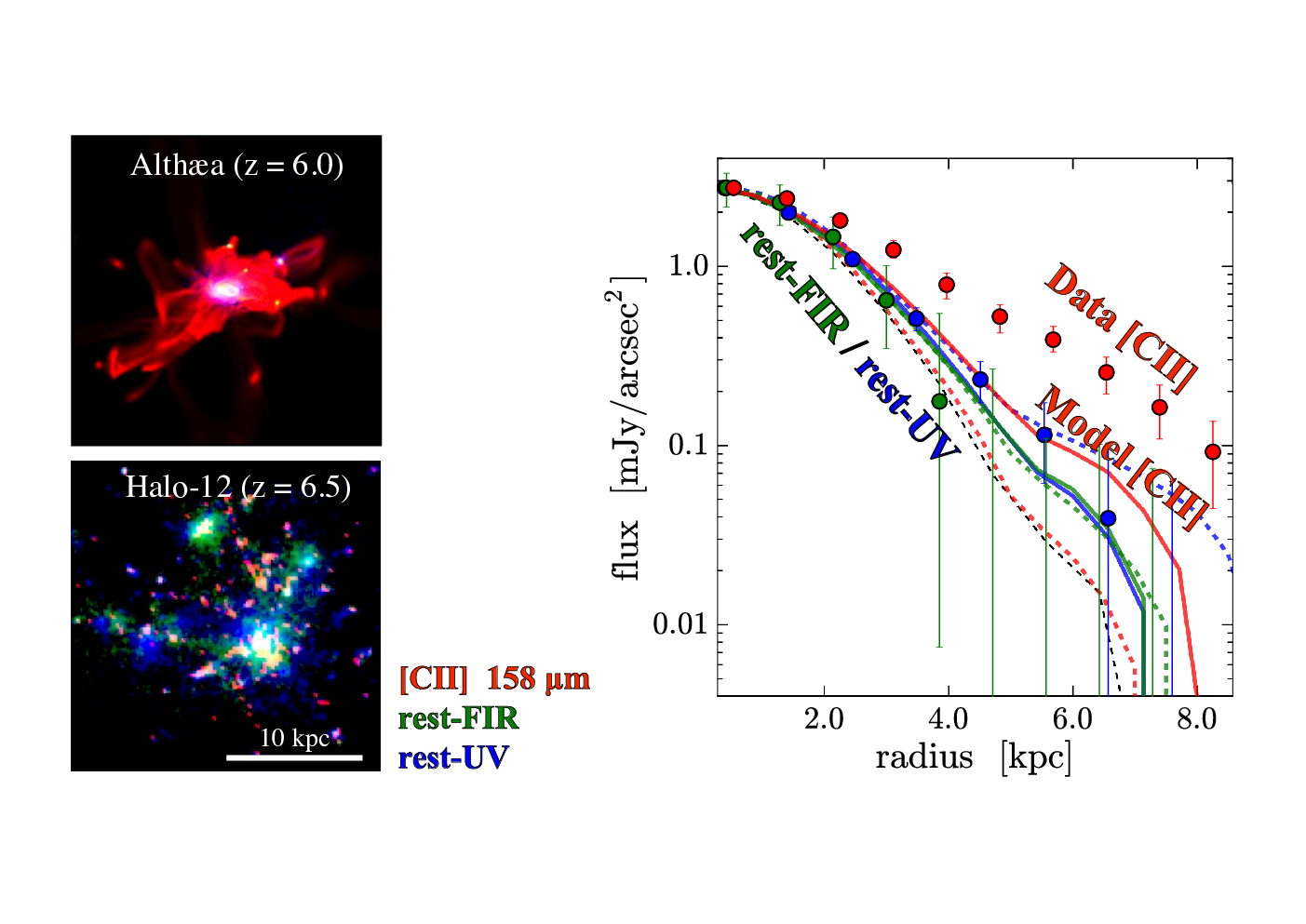
The left panel of Figure 11 presents a color composite of the [Cii] line, rest-frame UV, and FIR continuum emission of Altha at and Halo-12 at in the zoom-in simulations. The surface brightness morphology of the [Cii] line emission clearly shows the extended structure over the 10-kpc scale with surrounding satellite clumps and filamentary structures. The picture of the extended [C ii] halo around the central galaxies is roughly consistent with the observational results.
To quantitatively compare the zoom-in simulation to our observational results, we carry out the stacking for the zoom-in simulation results of the [C ii] line, the rest-frame FIR and the rest-frame UV continuum in the same manner as the observations. For the Altha simulation, we take 12 snapshots at different redshifts within For each snapshot, we calculate the surface brightness from face-on and three random angles, where the [C ii] line emissivity is calculated within 100 km s-1 of the velocity center of the galaxy to match the visibility-based stacking procedure for the ALMA data. In this way, we obtain 48 (=) images of Altha. We refer to Kohandel et al. 2019 for a full analysis of the different morphological results from different evolutionary stages and viewing angles. We then select 9 out of 48 snapshots randomly – the same sample size used for the stacking of the ALMA-HST sample. Finally, we perform the stacking of the intrinsic images, and smooth the stacked images with the ALMA beam. For the second set of simulation, we calculate the surface brightness from three orthogonal angles for four different halos (Halo-12, Halo-A, Halo-B, Halo-C) and obtain 12 (=) images. We then carry out the same stacking and smoothing procedures as the first simulation.
In the right panel of Figure 11, we show the radial surface brightness profiles estimated from the two independent zoom-in simulations. For comparison, we also plot the observational results obtained in Section IV. We find that both simulations reproduce the overall trend of observational results of rest-frame UV and FIR continuum within the errors. However, we also find that the [Cii] line emission in both simulations is not as extended as the observed data. In Altha, although it reproduces the trend that the [C ii] line is more extended than that of the rest-frame FIR and UV continuum, the intensity of the [C ii] emission at kpc is still lower than the observed one. In Halo-12, the [C ii] line is the least extended. These results indicate that the existence of the [C ii] halo challenges current hydrodynamic simulations of galaxy formation.
V. Discussion
In Section IV, we find that the [Cii] line emission is extended up to 10-kpc scale around the normal star-forming galaxies at and is potentially related to the Ly halo. In contrast to the previous reports of the 10-kpc-scale carbon reservoirs around rare, massive galaxies, such as dusty starbursts and quasars at –6 (Ivison et al. 2011; Falgarone et al. 2017; George et al. 2014; Díaz-Santos et al. 2014; Maiolino et al. 2012; Cicone et al. 2015, e.g.,), our results indicate that the cold carbon gas halo universally exists even around early normal galaxies.
The existence of the cold carbon gas halos around the early normal galaxies
raises two questions: what powers the [C ii] line emission
and how is the carbon abundance in the circum-galactic (CG) area
enriched at such early cosmic epochs.
Theoretical studies suggest the following five scenarios
that can give rise to the extended [C ii] line emission
with the potential association of the Ly halo:
A) satellite galaxies,
B) CG photodissociation region (PDR),
C) CG HII region,
D) cold streams,
E) outflow.
These five scenarios are illustrated in Figure 12.

The first scenario invokes satellite galaxies (Figure 12-A). If satellite galaxies exist around the central star-forming galaxies, the [Cii] and Ly line emission from the satellite galaxies will be observed as extended structures around the central galaxies. In this scenario, the extended halo size is determined by the spatial distribution of the satellite galaxies, which explains both extended components of the [Cii] and Ly line emission.
The second scenario is a PDR extended over CG scale, referred to as CG-PDR (Figure 12-B). The ionizing photons ( eV) from massive stars form the HII region on the central galactic scale. Far-ultraviolet (FUV) photons (6 eV eV) penetrate the surrounding ISM deeper than the ionizing photons, making the PDR more extended than the HII region. In these PDRs, the carbon is still singly ionized (11.3 eV) by the FUV photons. If the PDR is extended over the CG scale, the extended [Cii] line emission is thus detected on the CG scale. Besides, the Ly line emission is also spatially extended due to the resonant scattering by the neutral hydrogen in the surrounding ISM (Xue et al. 2017, e.g.,).
The third scenario is that ionizing photons penetrate the surrounding ISM deeper and form large HII regions even spreading over the CGM, which we refer to as CG-HII (Figure 12-C). This scenario is similar to scenario (B), but the existence of strong ionizing sources and/or ISM properties differ from scenario (B), and the HII region is larger than scenario (B) where the carbon is singly ionized. In this case, the Ly line emission is extended due to the fluorescence (Mas-Ribas & Dijkstra 2016, e.g.,), instead of the resonance scattering in scenario (B).
The fourth scenario is cold streams (Figure 12-D). Cosmological hydrodynamical simulations suggest that intense star-formation in high- galaxies is fed by a dense and cold gas (104 K) which is dubbed cold streams (Dekel et al. 2009, e.g.,). The cold streams radiate [Cii] as well as Ly line emission powered by gravitational energy, and produce the extended [Cii] and Ly line emission around a galaxy. Moreover, the cold stream may cause shock heating which can also produce the [Cii] and Ly line emission.
The fifth scenario is outflow (Figure 12-E). In the outflow, the ionized carbon and hydrogen powered by the AGN and/or star-formation feedback produce the extended [Cii] and Ly line emission (see also Faisst et al. 2017). The associated process of the shock heating may also contribute to radiating these line emission. Note that although we choose ALMA sources not reported as AGNs, we cannot rule out the possibility that our ALMA sources contain faint AGNs and/or have the past AGN activity.
In the following subsections, we discuss these possibilities based on the observational and theoretical results.
V.1. Hints From Observational Results
In the observational results, the [C ii] line is more extended than both the rest-frame FIR dust and UV continuum beyond the errors up to a radius of at least kpc (Figure 6). Assuming a constant [C ii] line emissivity at a given stellar continuum (De Looze et al. 2014), the large gap between the radial profiles of the [C ii] line and the stellar continuum indicates that the stellar continuum is not enough to explain the large part of the [C ii] line emissivity of the [C ii] halo.
Although the [C ii] line emissivity may be changed from the central to halo areas at a given stellar continuum, the metallicity at such outer areas is expected to be of the galaxy center (Pallottini et al. 2017a). Even if the stellar continuum in the outskirts is coming from low-mass, faint satellite galaxies, the massmetallicity relation (Mannucci et al. 2010) also suggests lower metallicities for the satellite galaxies. Because lower metallicity reduces the [C ii] line emissivity for a given stellar continuum (Vallini et al. 2015), it would be difficult to explain the [C ii] halo by the same source as the stellar continuum. In fact, Figure 8 shows that the /SFRtotal ratio becomes higher towards outskirts of the halo, which cannot be explained by the dwarf galaxies. Our observational results thus rule out scenario (A), and support the other four scenarios.
In the recent [Cii] line studies at , Gallerani et al. 2018 report signatures of starburst-driven outflows from 9 normal star-forming galaxies at with the stacked [Cii] spectra. With the similar sample, the rest-frame UV metal absorptions are also identified to be blue-shifted from the [C ii]-systemic redshift in the stacked Keck spectra (Sugahara et al. 2019). From more luminous objects, the broad wing features are detected in the stacked [C ii] line spectra of quasars (Bischetti et al. 2018) as well as in an individual [C ii] line spectrum of a quasar at (Maiolino et al. 2012; Cicone et al. 2015). These recent results suggest that scenario (E) may be potentially very interesting. However, it is also reported that the stacked [Cii] spectra even from 23 quasars at shows no clear evidence of the existence of strong feedback (Decarli et al. 2018). Also, our stacked [C ii] spectra with the 18 star-forming galaxies does not show a clear broad wing feature, neither (Section IV.5). Among scenarios of (B), (C), (D), and (E), we thus cannot conclude the most likely one from our and recent observational results.
V.2. Hints From Theoretical Results
In the simulation results, the extended profile of [C ii] halo is not fully reproduced (Figure 11). This may suggest that some physical processes are not sufficiently solved in the simulations, e.g., metal enrichment, feedback, ISM/CGM clumpiness, and the propagation of ionizing radiation. On the other hand, if the current assumptions related to the [C ii] line emissivity are correct, additional mechanism(s) are required to produce the extended [C ii] line emissivity in the simulation.
There are two possibilities for such additional mechanisms that are not included in the calculation of the [C ii] line emissivity in the simulations. The first possible mechanism is the shock heating; Appleton et al. 2013 have shown that [C ii] can be excited on large scales from the dissipation of mechanical energy of galaxy mergers via turbulent cascade. Although the shock heating should be captured in the hydrodynamical calculation of the zoom-in simulation, it is possible that the current simulations do not have sufficient resolution to capture the turbulent cascade of large-scale mechanical energy down to the molecular cloud scales. This means that the computation of the ionized carbon abundance in cloudy does not adequately consider the effect of shock heating. Since shock heating is caused by galaxy merger or gas inflow/outflow processes, the [C ii] emissivity could become more enhanced if the shock heating and associated turbulent cascade is properly treated in the scenarios (A), (D), and (E).
The second possible mechanism is the past/on-going AGN activities, which could form a large HII region and surrounding PDR. Moreover, the AGN feedback may cause shock heating, which also could contribute to the [C ii] line emissivity. In this case, the scenarios of (C) and (E) are further supported.
Note that if the effect of shocks and AGNs is too strong, the carbon may be doubly ionized, and then the [C ii] line is rarely emitted. Therefore, it is hard to conclude whether the missing treatment of shocks and/or AGNs in current simulations are the major causes of the inadequate [C ii] halo in the simulations.
It should also be noted that 7 out of 9 sources in the ALMA-HST sample are placed at when the effect of CMB is weaker than at , from which the zoom-in simulation results were taken. Because the CMB effect reduces the line luminosity from the diffuse component (da Cunha et al. 2013; Zhang et al. 2016; Pallottini et al. 2015; Lagache et al. 2018, e.g.,), the slight difference in the redshift range may cause the insufficient [Cii] line luminosity in the zoom-in simulation results.
V.3. Physical Origin of [Cii]Halo
We summarize the possible scenarios of what powers the [Cii] halo based on the results of Sections V.1V.2. From the observational results, we rule out scenario (A). In the zoom-in simulation results, it is hard to conclude which scenario is the most plausible one unless we perform further analyses with different models of SN and AGN feedback, for example. The possible scenarios at this point are thus (B), (C), (D), and (E) given the current best estimates of both observational and theoretical results.
Most importantly, the outflow activities are required in all cases to enrich the CGM with carbon around the normal star-forming galaxies in the early Universe. Our results are thus the evidence of outflow remnants in these early star-forming galaxies.
There are two modes of outflows, hot-mode and cold-mode outflows (Murray et al. 2011; Hopkins et al. 2014; Muratov et al. 2015; Heckman & Thompson 2017, e.g.,). The hot-mode outflow is defined as the outflow of ionized hydrogen (hot) gas that is heated by supernova (SN) explosions, massive star/AGN radiation. Since the cooling time of such hot gas ( K) can be longer than the cosmic time at 57 (1 Gyr; e.g., Madau et al. 2001), it would be difficult to produce the [C ii]-emitting cold halos from the hot-mode outflow. On the other hand, the cold-mode outflow consists of the cold neutral hydrogen gas that is pushed by the radiative and kinetic pressures exerted by SNe, massive stars, and AGNs. In this case, the majority of [Cii] line emission would be radiated from the PDR in the cold, neutral hydrogen gas clouds. Therefore our finding of the [Cii] halo suggests that outflows in the early star-forming galaxies may be dominated by the cold-mode outflows.
Since we also find the similarity in the radial surface brightness profiles between the [Cii] and Ly halos (Figure 9), the physical origin of the [Cii] halo may be related to the Ly halo. Future deep observations of both [Cii] and Ly line emission for individual high- galaxies are required to comprehensively understand the mechanism of the CGM metal enrichment with the theoretical simulations including the radiative transfers of these line emission.
VI. Summary
In this paper, we study the detailed morphology of [Cii] line emission via the ALMA visibility-based stacking method for normal star-forming galaxies whose [Cii] line have been individually detected at . The visibility-based stacking achieves deep and well-sampled visibility data in the -plane, which enables us to securely investigate the diffuse emission extended over the circum-galactic environment. In conjunction with the deep HST/-band data, we examine the radial surface brightness profiles of the [Cii] line, rest-frame FIR, and UV continuum emission. We then discuss the physical origin of the extended [Cii] line emission. The major findings of this paper are summarized below.
- 1.
The visibility-based stacking of our and archival deep ALMA data for 18 galaxies with SFR 1070 yr-1 at produces 21 and 10 level detections at the peak for the [Cii] line and dust continuum emission, respectively. The stacked [Cii] line morphology is spatially extended more than that of the dust continuum. The radial surface brightness profiles of the [Cii] line are extended up to a radius of 10-kpc scale at the 9.2 level.
- 2.
The HST/-band stacking for 9 out of the 18 [Cii] line sources that are taken by the deep HST observations shows that the radial surface brightness profiles of the [Cii] line is significantly extended more than that of the rest-frame UV as well as the rest-frame FIR continuum emission. We derive the radial ratio of /SFRtotal, showing that the ratio becomes higher towards the outskirts of halo where the high ratios cannot be explained by the satellite galaxies.
- 3.
The two-component Srsic+exponential profile fitting results indicate that the extended [Cii] halo component has the scale length of 3.3 0.1 kpc, which is comparable to the Ly halo, universally found around the high- star-forming galaxies. In terms of effective radius, the extended [Cii] halo component is larger than the central galactic component by a factor of 5.
- 4.
The state-of-the-art zoom-in cosmological hydrodynamic simulations roughly reproduce the radial surface brightness profile trends of the extended [Cii] line emission and the rest-frame FIR, comparable to the rest-frame UV continuum emission. However, the simulations do not reproduce the full extent of the [Cii] halo in the outskirts, where the simulations might be missing some physical mechanisms associated with the feedback, or still lacking the resolution to resolve the turbulent cascade from large-scale shocks down to the small scales of molecular clouds, if such a process is indeed important for the [C ii] emission in high- galaxies as Appleton et al. 2013 argued.
- 5.
Although there remain several possible scenarios that can give rise to [C ii] line emission in the CGM, the outflow is required in any cases to enrich the primordial CGM with carbon around the early star-forming galaxies. Our results are thus the evidence of outflow remnants in the early star-forming galaxies and suggest that the outflow may be dominated by the cold-mode outflow.
We thank the anonymous referee for constructive comments and suggestions. We are grateful to Ivan Marti-Vidal and the Nordic ALMA Regional Center for providing us with helpful CASA software tools and advice on analyzing the data. We appreciate Tohru Nagao, Jeremy Blaizot, Peter Mitchell, Takashi Kojima, Shiro Mukae, Yuichi Harikane, Akio Inoue, and Rieko Momose for useful comments and suggestions. We are indebted for the support of the staff at the ALMA Regional Center. This paper makes use of the following ALMA data: ADS/JAO. ALMA #2013.1.00815.S, #2015.1.00834.S, #2015.1.01111.S, #2015.1.01105, #2016.1.01240.S, #2012.1.00523.S, and #2012.1.00602.S. ALMA is a partnership of the ESO (representing its member states), NSF (USA) and NINS (Japan), together with NRC (Canada), MOST and ASIAA (Taiwan), and KASI (Republic of Korea), in cooperation with the Republic of Chile. The Joint ALMA Observatory is operated by the ESO, AUI/NRAO, and NAOJ. This study is supported by World Premier International Research Center Initiative (WPI Initiative), MEXT, Japan, and KAKENHI (15H02064, 16J02344, 17H01110, 17H01111, and 17H01114) Grant-in-Aid for Scientific Research (A) through Japan Society for the Promotion of Science (JSPS), the Grant-in-Aid for JSPS Research Fellow, the NAOJ ALMA Scientific Research Grant Number 2017-06B, and the Munich Institute for Astro- and Particle Physics (MIAPP) of the DFG cluster of excellence ”Origin and Structure of the Universe”. S.F. is supported by the ALMA Japan Research Grant of NAOJ Chile Observatory NAOJ-ALMA-197, The 2018 Graduate Research Abroad in Science Program Grant (GRASP2018), and the Hayakawa Satio Fund awarded by the Astronomical Society of Japan, and NAOJ ALMA Scientific Research Grant Number 2016-01A. A.F. and R.J.I acknowledge supports from the ERC Advanced Grant INTERSTELLAR H2020/740120 and COSMIC ISM 321302, respectively.
Appendix A Our ALMA Sample
The sources drawn from the literature in our ALMA sample is summarized in Table 1.
For this literature sample, Figure 13 shows the [C ii] line velocity-integrated maps and
the spectra obtained from our re-analysis of the archival ALMA data.
We confirm that the spatial morphology and the spectrum shape of the [C ii] lines are consistent with the previous studies
(Capak et al. 2015; Willott et al. 2015; Pentericci et al. 2016; Smit et al. 2018; Carniani et al. 2018).

![[Uncaptioned image]](1902.06760v4/postage2.png)
Figure 13. (continued)
References
- Appleton et al. (2013) Appleton, P. N., Guillard, P., Boulanger, F., et al. 2013, ApJ, 777, 66
- Arata et al. (2019a) Arata, S., Yajima, H., Nagamine, K., Li, Y., & Khochfar, S. 2019a, arXiv e-prints, arXiv:1908.01438
- Arata et al. (2019b) —. 2019b, MNRAS, 488, 2629
- Aravena et al. (2016) Aravena, M., Decarli, R., Walter, F., et al. 2016, ApJ, 833, 71
- Barisic et al. (2017) Barisic, I., Faisst, A. L., Capak, P. L., et al. 2017, ApJ, 845, 41
- Behrens et al. (2018) Behrens, C., Pallottini, A., Ferrara, A., Gallerani, S., & Vallini, L. 2018, MNRAS, 477, 552
- Bertin & Arnouts (1996) Bertin, E., & Arnouts, S. 1996, A&A, 117, 393
- Bischetti et al. (2018) Bischetti, M., Maiolino, R., Fiore, S. C. F., Piconcelli, E., & Fluetsch, A. 2018, ArXiv e-prints, arXiv:1806.00786
- Bouwens et al. (2017) Bouwens, R. J., van Dokkum, P. G., Illingworth, G. D., et al. 2017, ArXiv e-prints, arXiv:1711.02090
- Capak et al. (2015) Capak, P. L., Carilli, C., Jones, G., et al. 2015, Nature, 522, 455
- Carniani et al. (2017) Carniani, S., Maiolino, R., Amorin, R., et al. 2017, ArXiv e-prints, arXiv:1712.03985
- Carniani et al. (2018) —. 2018, MNRAS, arXiv:1712.03985
- Cicone et al. (2015) Cicone, C., Maiolino, R., Gallerani, S., et al. 2015, A&A, 574, A14
- Coppin et al. (2008) Coppin, K., Halpern, M., Scott, D., et al. 2008, MNRAS, 384, 1597
- Cullen et al. (2017) Cullen, F., McLure, R. J., Khochfar, S., Dunlop, J. S., & Dalla Vecchia, C. 2017, MNRAS, 470, 3006
- da Cunha et al. (2013) da Cunha, E., Groves, B., Walter, F., et al. 2013, ApJ, 766, 13
- De Looze et al. (2014) De Looze, I., Cormier, D., Lebouteiller, V., et al. 2014, A&A, 568, A62
- Decarli et al. (2018) Decarli, R., Walter, F., Venemans, B. P., et al. 2018, ApJ, 854, 97
- Dekel et al. (2009) Dekel, A., Birnboim, Y., Engel, G., et al. 2009, Nature, 457, 451
- Díaz-Santos et al. (2014) Díaz-Santos, T., Armus, L., Charmandaris, V., et al. 2014, ApJ, 788, L17
- Dunlop et al. (2017) Dunlop, J. S., McLure, R. J., Biggs, A. D., et al. 2017, MNRAS, 466, 861
- Faisst et al. (2017) Faisst, A. L., Capak, P. L., Yan, L., et al. 2017, ApJ, 847, 21
- Falgarone et al. (2017) Falgarone, E., Zwaan, M. A., Godard, B., et al. 2017, Nature, 548, 430
- Ferland et al. (2017) Ferland, G. J., Chatzikos, M., Guzmán, F., et al. 2017, Rev. Mexicana Astron. Astrofis., 53, 385
- Fujimoto et al. (2016) Fujimoto, S., Ouchi, M., Ono, Y., et al. 2016, ApJS, 222, 1
- Fujimoto et al. (2017) Fujimoto, S., Ouchi, M., Shibuya, T., & Nagai, H. 2017, ApJ, 850, 1
- Fujimoto et al. (2018) Fujimoto, S., Ouchi, M., Kohno, K., et al. 2018, ApJ, 861, 7
- Gaia Collaboration et al. (2018) Gaia Collaboration, Brown, A. G. A., Vallenari, A., et al. 2018, A&A, 616, A1
- Gallerani et al. (2018) Gallerani, S., Pallottini, A., Feruglio, C., et al. 2018, MNRAS, 473, 1909
- George et al. (2014) George, R. D., Ivison, R. J., Smail, I., et al. 2014, MNRAS, 442, 1877
- Harikane et al. (2018) Harikane, Y., Ouchi, M., Ono, Y., et al. 2018, PASJ, 70, S11
- Hashimoto et al. (2018) Hashimoto, T., Inoue, A. K., Mawatari, K., et al. 2018, arXiv e-prints, arXiv:1806.00486
- Hayatsu et al. (2017) Hayatsu, N. H., Matsuda, Y., Umehata, H., et al. 2017, PASJ, 69, 45
- Heckman & Thompson (2017) Heckman, T. M., & Thompson, T. A. 2017, Galactic Winds and the Role Played by Massive Stars, ed. A. W. Alsabti & P. Murdin, 2431
- Hodge et al. (2016) Hodge, J. A., Swinbank, A. M., Simpson, J. M., et al. 2016, ApJ, 833, 103
- Hopkins et al. (2014) Hopkins, P. F., Kereš, D., Oñorbe, J., et al. 2014, MNRAS, 445, 581
- Ikarashi et al. (2015) Ikarashi, S., Ivison, R. J., Caputi, K. I., et al. 2015, ApJ, 810, 133
- Ilbert et al. (2013) Ilbert, O., McCracken, H. J., Le Fèvre, O., et al. 2013, A&A, 556, A55
- Ivison et al. (2011) Ivison, R. J., Papadopoulos, P. P., Smail, I., et al. 2011, MNRAS, 412, 1913
- Johnson et al. (2013) Johnson, J. L., Dalla Vecchia, C., & Khochfar, S. 2013, MNRAS, 428, 1857
- Jones et al. (2017) Jones, G. C., Willott, C. J., Carilli, C. L., et al. 2017, ApJ, 845, 175
- Kawamata et al. (2018) Kawamata, R., Ishigaki, M., Shimasaku, K., et al. 2018, ApJ, 855, 4
- Knudsen et al. (2016) Knudsen, K. K., Richard, J., Kneib, J.-P., et al. 2016, MNRAS, 462, L6
- Kohandel et al. (2019) Kohandel, M., Pallottini, A., Ferrara, A., et al. 2019, MNRAS, 487, 3007
- Lagache et al. (2018) Lagache, G., Cousin, M., & Chatzikos, M. 2018, A&A, 609, A130
- Leclercq et al. (2017) Leclercq, F., Bacon, R., Wisotzki, L., et al. 2017, A&A, 608, A8
- Li et al. (2008) Li, Y., Hopkins, P. F., Hernquist, L., et al. 2008, ApJ, 678, 41
- Lindroos et al. (2015) Lindroos, L., Knudsen, K. K., Vlemmings, W., Conway, J., & Martí-Vidal, I. 2015, MNRAS, 446, 3502
- Madau et al. (2001) Madau, P., Ferrara, A., & Rees, M. J. 2001, ApJ, 555, 92
- Maiolino et al. (2012) Maiolino, R., Gallerani, S., Neri, R., et al. 2012, MNRAS, 425, L66
- Maiolino et al. (2015) Maiolino, R., Carniani, S., Fontana, A., et al. 2015, MNRAS, 452, 54
- Mannucci et al. (2010) Mannucci, F., Cresci, G., Maiolino, R., Marconi, A., & Gnerucci, A. 2010, MNRAS, 408, 2115
- Martí-Vidal et al. (2014) Martí-Vidal, I., Vlemmings, W. H. T., Muller, S., & Casey, S. 2014, A&A, 563, A136
- Mas-Ribas & Dijkstra (2016) Mas-Ribas, L., & Dijkstra, M. 2016, ApJ, 822, 84
- Matsuda et al. (2012) Matsuda, Y., Yamada, T., Hayashino, T., et al. 2012, MNRAS, 425, 878
- Matthee et al. (2015) Matthee, J., Sobral, D., Santos, S., et al. 2015, MNRAS, 451, 400
- Matthee et al. (2017) Matthee, J., Sobral, D., Boone, F., et al. 2017, ApJ, 851, 145
- McMullin et al. (2007) McMullin, J. P., Waters, B., Schiebel, D., Young, W., & Golap, K. 2007, in Astronomical Society of the Pacific Conference Series, Vol. 376, Astronomical Data Analysis Software and Systems XVI, ed. R. A. Shaw, F. Hill, & D. J. Bell, 127
- Momose et al. (2014) Momose, R., Ouchi, M., Nakajima, K., et al. 2014, MNRAS, 442, 110
- Momose et al. (2016) —. 2016, MNRAS, 457, 2318
- Muratov et al. (2015) Muratov, A. L., Kereš, D., Faucher-Giguère, C.-A., et al. 2015, MNRAS, 454, 2691
- Murphy et al. (2011) Murphy, E. J., Condon, J. J., Schinnerer, E., et al. 2011, ApJ, 737, 67
- Murray et al. (2011) Murray, N., Ménard, B., & Thompson, T. A. 2011, ApJ, 735, 66
- Oesch et al. (2010) Oesch, P. A., Bouwens, R. J., Carollo, C. M., et al. 2010, ApJ, 725, L150
- Oke & Gunn (1983) Oke, J. B., & Gunn, J. E. 1983, ApJ, 266, 713
- Ono et al. (2013) Ono, Y., Ouchi, M., Curtis-Lake, E., et al. 2013, ApJ, 777, 155
- Ouchi et al. (2008) Ouchi, M., Shimasaku, K., Akiyama, M., et al. 2008, ApJS, 176, 301
- Ouchi et al. (2009) Ouchi, M., Mobasher, B., Shimasaku, K., et al. 2009, ApJ, 706, 1136
- Ouchi et al. (2010) Ouchi, M., Shimasaku, K., Furusawa, H., et al. 2010, ApJ, 723, 869
- Pallottini et al. (2017a) Pallottini, A., Ferrara, A., Bovino, S., et al. 2017a, MNRAS, 471, 4128
- Pallottini et al. (2017b) Pallottini, A., Ferrara, A., Gallerani, S., et al. 2017b, MNRAS, 465, 2540
- Pallottini et al. (2015) Pallottini, A., Gallerani, S., Ferrara, A., et al. 2015, MNRAS, 453, 1898
- Peng et al. (2010) Peng, C. Y., Ho, L. C., Impey, C. D., & Rix, H.-W. 2010, AJ, 139, 2097
- Pentericci et al. (2016) Pentericci, L., Carniani, S., Castellano, M., et al. 2016, ApJ, 829, L11
- Planck Collaboration et al. (2011) Planck Collaboration, Abergel, A., Ade, P. A. R., et al. 2011, A&A, 536, A21
- Rujopakarn et al. (2016) Rujopakarn, W., Dunlop, J. S., Rieke, G. H., et al. 2016, ApJ, 833, 12
- Rybak et al. (2019) Rybak, M., Calistro Rivera, G., Hodge, J. A., et al. 2019, ApJ, 876, 112
- Schaye et al. (2010) Schaye, J., Dalla Vecchia, C., Booth, C. M., et al. 2010, MNRAS, 402, 1536
- Sérsic (1963) Sérsic, J. L. 1963, Boletin de la Asociacion Argentina de Astronomia La Plata Argentina, 6, 41
- Shibuya et al. (2015) Shibuya, T., Ouchi, M., & Harikane, Y. 2015, ApJS, 219, 15
- Simpson et al. (2015) Simpson, J. M., Smail, I., Swinbank, A. M., et al. 2015, ApJ, 799, 81
- Skelton et al. (2014) Skelton, R. E., Whitaker, K. E., Momcheva, I. G., et al. 2014, ApJS, 214, 24
- Smit et al. (2015) Smit, R., Bouwens, R. J., Franx, M., et al. 2015, ApJ, 801, 122
- Smit et al. (2018) Smit, R., Bouwens, R. J., Carniani, S., et al. 2018, Nature, 553, 178
- Springel (2005) Springel, V. 2005, MNRAS, 364, 1105
- Stacey et al. (1991) Stacey, G. J., Geis, N., Genzel, R., et al. 1991, ApJ, 373, 423
- Steidel et al. (2011) Steidel, C. C., Bogosavljević, M., Shapley, A. E., et al. 2011, ApJ, 736, 160
- Sugahara et al. (2019) Sugahara, Y., Ouchi, M., Harikane, Y., et al. 2019, arXiv e-prints, arXiv:1904.03106
- Vallini et al. (2015) Vallini, L., Gallerani, S., Ferrara, A., Pallottini, A., & Yue, B. 2015, ApJ, 813, 36
- Venemans et al. (2019) Venemans, B. P., Neeleman, M., Walter, F., et al. 2019, ApJ, 874, L30
- Watson et al. (2015) Watson, D., Christensen, L., Kraiberg Knudsen, K., et al. 2015, ArXiv e-prints, arXiv:1503.00002
- Willott et al. (2015) Willott, C. J., Carilli, C. L., Wagg, J., & Wang, R. 2015, ApJ, 807, 180
- Willott et al. (2013a) Willott, C. J., Omont, A., & Bergeron, J. 2013a, ApJ, 770, 13
- Willott et al. (2013b) Willott, C. J., McLure, R. J., Hibon, P., et al. 2013b, AJ, 145, 4
- Xue et al. (2017) Xue, R., Lee, K.-S., Dey, A., et al. 2017, ApJ, 837, 172
- Yajima et al. (2012) Yajima, H., Li, Y., Zhu, Q., & Abel, T. 2012, MNRAS, 424, 884
- Yajima et al. (2017) Yajima, H., Nagamine, K., Zhu, Q., Khochfar, S., & Dalla Vecchia, C. 2017, ApJ, 846, 30
- Zhang et al. (2016) Zhang, Z.-Y., Papadopoulos, P. P., Ivison, R. J., et al. 2016, Royal Society Open Science, 3, 160025