Exotic compact object behavior in black hole analogues

The draining bathtub geometry introduced by Visser Visser 1998 describes the irrotational flow of a barotropic and inviscid fluid with background density $\rho_{0}$ in a plane with a sink at the origin. The irrotational nature of the flow together with the conservation of angular momentum require the background density to be constant, i.e. position-independent. As a result, the background pressure $p_{0}$ and the speed of sound $c$ are also constant throughout the flow. Furthermore, it follows from both the equation of continuity and the conservation of angular momentum that the unperturbed velocity profile $\mathbf{v}_{0}$ of the flowing fluid is given in polar coordinates $(r,\phi)$ by

with $v_{0}^{(r)}=-A/r$ and $v_{0}^{(\phi)}=B/r$, where $A,B\in\mathbb{R}^{+}$. $\mathbf{e}_{r}$ and $\mathbf{e}_{\phi}$ are the radial and azimuthal unit vectors, respectively. A general velocity profile $\mathbf{v}$, allowing for perturbations, can be written as the gradient of a velocity potential $\Psi$, i.e. $\mathbf{v}=\nabla\Psi$. When $\mathbf{v}=\mathbf{v}_{0}$, $\Psi=\Psi_{0}(r,\theta)\equiv A\log r+B\phi$ (apart from a constant of integration).

In polar coordinates $(t,r,\phi)$, the line element of the draining bathtub model has the form Schützhold and Unruh 2002; Visser and Weinfurtner 2005

where the constant prefactor $(\rho_{0}/c)^{2}$ has been omitted. Eq. (2) has the Painlevé-Gullstrand form Berti 2005.

The flow is stationary and axisymmetric, i.e. the metric tensor in Eq. (2) does not depend explicitly on $t$ nor on $\phi$. In polar coordinates, the Killing vectors associated with these continuous symmetries are $\bm{\xi}_{t}\equiv\partial_{t}$ and $\bm{\xi}_{\phi}\equiv\partial_{\phi}$, respectively. This geometry has an acoustic horizon located at $r=r_{H}\equiv A/c$ and a region of transonic flow defined by $r_{H}<r<r_{E}$, where $r_{E}=\sqrt{A^{2}+B^{2}}/c$ is the location of the ergosphere¹¹ 1 The speed of the flowing fluid is $\phi-$independent and given by $v_{0}\equiv\|\mathbf{v}_{0}\|=\sqrt{A^{2}+B^{2}}/r$. It equals the speed of sound at $r=r_{E}$ and exceeds it everywhere in the region $r_{H}<r<r_{E}$..

Performing the coordinate transformation

one can cast Eq. (2) in the form Basak and Majumdar 2003b; Berti et al. 2004; Dolan and Oliveira 2013

where

The coordinates $(\tilde{t},r,\tilde{\phi})$ are equivalent to the Boyer-Lindquist coordinates commonly used to write the Kerr metric.

The numerical results to be presented in the following were obtained using a direct-integration method. The integration of Eq. (19) is performed using the numerically convenient expansions

for the radial function $H_{\omega m}(r)$ in Eq. (II.2.3) in the near and in the far regions, respectively, where

Note that $\tilde{H}_{h}(r_{0})\approx(1+\underline{\mathcal{R}}\delta^{+i\varpi})\delta^{-i\varpi/2}$. According to Eq. (II.2.3), $H_{\omega m}(r_{0})\sim(1+\mathcal{R})e^{-i\varpi r_{0}^{*}}$, meaning that one should require⁴⁴ 4 Using Eq. (17), one can show that $e^{-i\varpi r_{0}^{*}}=e^{-i\varpi r_{0}}\left(\frac{\delta}{\delta+2}\right)^{-i\varpi/2}\sim\delta^{-i\varpi/2}$, where the last step holds as long as $\delta\ll 1$. $\tilde{H}_{h}(r_{0})\sim(1+\mathcal{R})\delta^{-i\varpi/2}$, from which follows that $\underline{\mathcal{R}}=\mathcal{R}\delta^{-i\varpi}$. $N_{h}$ and $N_{\infty}$ are the number of terms of the partial sums. The coefficients $c_{n}$ and $d_{n}$ are functions of $\varpi$ and $\omega$, respectively, and both depend on $B$ and $m$. Inserting each expansion into Eq. (19) and equating coefficients order by order, it is possible to write $c_{1},\ldots,c_{N_{h}}$ ($d_{1},\ldots,d_{N_{\infty}}$) in terms of $c_{0}$ ($d_{0}$) . The latter is usually set to $1$. The choice of $N_{h}$ and/or $N_{\infty}$ should be a trade-off between computational time and accuracy. If the goal is to compute QNM frequencies, one assigns a guess value to $\omega$ and integrates Eq. (19) from $r=r_{\infty}$ to $r=r_{0}$ using the ansatz $\tilde{H}_{\infty}$ with $A_{s}^{-}=0$ so that the solution satisfies the relations $\tilde{H}_{\infty}=H_{\omega m}$ and $\mathrm{d}\tilde{H}_{\infty}/\mathrm{d}r=\mathrm{d}H_{\omega m}/\mathrm{d}r$ at $r=r_{\infty}$, where $r_{\infty}$ stands for the numerical value of infinity. The previous step is repeated for different guess values of $\omega$ until the solution satisfies the BC in Eq. (37) (one-parameter shooting). If the algorithm is numerically stable, variations in $N_{\infty}$ and/or $r_{\infty}$ do yield similar results. On the other hand, if the aim is to estimate the amplification factors defined in Eq. (35) for a given frequency $\omega$, one integrates Eq. (19) from $r=r_{0}$ to $r=r_{\infty}$ using the ansatz $\tilde{H}_{h}$ so that the solution satisfies the relations $\tilde{H}_{h}=H_{\omega m}$ and $\mathrm{d}\tilde{H}_{h}/\mathrm{d}r=\mathrm{d}H_{\omega m}/\mathrm{d}r$ at $r=r_{0}$ and then extracts the coefficients $A_{s}^{\pm}$ of the ansatz $\tilde{H}_{\infty}$ at infinity.

All numerical integrations were performed using the integration parameters $N_{h}=4$ and $N_{\infty}=10$. When computing QNM frequencies (amplification factors), $r_{\infty}$ was set to $100$ ($400$). The guess values to the QNM frequencies were chosen according to the numerical results reported in Maggio et al. 2017.

Fig. 1shows the fundamental $m=1$ QNM frequencies of perfectly-reflecting ECO-like vortices with different characteristic parameters⁵⁵ 5 Since $\delta\ll 1$, $\delta$ is a more suitable parameter than $r_{0}$. $\{\delta,B\}$ for DBCs ($\mathcal{R}=-1$) and NBCs ($\mathcal{R}=1$). Note that the bottom panels are plots of the absolute value of $\omega_{I}$. As pointed out in Sec. II, $\omega_{R}$ depends on $\arg(\mathcal{R})$ but not on $|\mathcal{R}|^{2}$. This means that the top panels of Fig. 1 give information about the real part of the QNM frequencies of both perfectly- and partially-reflecting ECO-like vortices.

The results are qualitatively similar for both BCs. At first order in $B$ (i.e. for $B\lesssim 0.1$), $\omega_{R}$ is a linear function of the angular velocity $B$, as one would expect from Eq. (38). The initial value (corresponding to $B=0$) depends on $r_{0}^{*}$ or, more precisely, on the the inverse of $\log\delta$, in accordance with Eq. (17). Similarly, $\omega_{I}$ grows monotonically with increasing rotation. Both $\omega_{R}$ and $\omega_{I}$ change sign from negative to positive as $B$ increases. Within numerical accuracy, the sign changes occur at the same critical value $B_{c}$, meaning $\omega_{R},\omega_{I}<0$ when $B<B_{c}$ and $\omega_{R},\omega_{I}>0$ when $B>B_{c}$. In other words, QNMs turn from stable to unstable as the fluid spins faster and faster and, furthermore, perfectly-reflecting ECO-like vortices admit zero-frequency ($\omega=0$) QNMs. Similar phenomenological aspects regarding the interaction of massless bosonic fields with perfectly-reflecting Kerr-like ECOs have been reported in Maggio et al. 2017; Hod 2017a; Maggio et al.. It was shown in particular that some ECOs or ECO analogues can only support static configurations of a scalar field for a discrete set of critical radii Hod 2017a; Hod 2017b; Hod 2017c; Hod 2018. This also holds true for the present case, as shown in the Appendix B.

The aforementioned instability finds its origin in the possible existence of negative-energy physical states inside the ergoregion. In general, in BH physics, the absence of an event horizon turns horizonless rotating ECOs unstable Friedman 1978; Maggio et al. 2017. The event horizon of Kerr BHs, which can be regarded as a perfectly-absorbing surface ($\mathcal{R}=0$), prevents the falling into lower and lower negative-energy states. The same does not occur when considering perfectly-reflecting BCs, hence the development of instabilities.

All the positive frequencies in the top panels of Fig. 1 refer to exponentially growing modes which meet the superradiance condition, that is to say that acoustic perturbations with such frequencies are amplified ($Z>0$) when scattered off perfectly-reflecting ECO-like vortices, thanks to the transfer of angular momentum and energy from the latter to the former. According to Eq. (41), only the absence of superradiant amplification when $\mathcal{R}=0$ ($Z_{0}<0$) guarantees exponentially decaying responses of perfectly-reflecting ($|\mathcal{R}|^{2}=1$) ECOs to external linear perturbations. From a dynamical point of view, the instability is expected to result in the scatterer spinning slower and slower until its fundamental QNM mode, whose frequency depends on $B$, starts decaying rather than growing over time, which occurs when $B=B_{c}$ (note that $Z<0$ when $B<B_{c}$). The instability domain of ECO-like vortices is depiected in Fig. 2. The threshold decreases monotonically as $r_{0}\rightarrow r_{H}$ (i.e. as $\delta\rightarrow 0$).

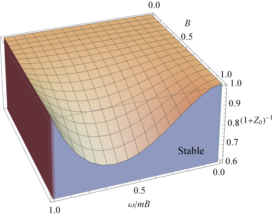
Is there any way of preventing ECO-like vortices from developing instabilities without changing $B$? The answer is affirmative. In the presence of superradiance ($Z_{0}>0$), unless $B<B_{c}$, it is clear that only partially-reflecting ECO-like vortices may be stable. However, attention must be paid to the fact that an ECO with $|\mathcal{R}|^{2}<1$ is not perforce dynamically stable. In fact, for each frequency satisfying the superradiance condition, there is a range of values $|\mathcal{R}|^{2}$ can take to assure stability. Using the small-frequency approximations in Eqs. (57) and (58), Eq. (41) takes the explicit form

where $\chi=\beta(\beta-m)^{-1}\prod_{n=0}^{m-1}(\beta-m+n)^{2}$. The upper bound on $|\mathcal{R}|^{2}$ represents the threshold for the manifestation of ergoregion instabilities and depends both on $\omega$ and $B$, as shown in Fig. 3.

One is interested in setting restrictions on $|\mathcal{R}|^{2}$ which are frequency-independent, in order to avert exponentially growing linear perturbations regardless of their frequency. The absolute upper bound on $|\mathcal{R}|^{2}$ from Eq. (41), herein dubbed maximum reflectivity, is set by the maximum amplification factor when $\mathcal{R}=0$, i.e. to the minimum of the function $(1+Z_{0})^{-1}$, and is therefore independent of $\delta$. For sufficiently slow drains ($B\leq 1$), ECO-like vortices are stable against acoustic perturbations of any frequency as long as $|\mathcal{R}|^{2}\lesssim 70\%$.

Fig. 4illustrates the amplification factors for superradiant $m=1$ acoustic linear perturbations scattered off ECO-like vortices with $\delta=10^{-6}$, $B=0.6$ and different reflectivities. The numerical results were obtained via the direct-integration method described previously, whereas the analytical ones were computed using the small-frequency approximations in Eqs. (57) and (58) via Eq. (60). The closeness between numerical and analytical results is evident. The data for different reflectivities share some qualitatively features: the amplification factors appear to vanish at the endpoints of the superradiant regime (i.e. at $\omega=0$ and $\omega=mB$) and have a maximum value. The graph referring to the draining bathtub ($\mathcal{R}=0$) is in agreement with numerical results previously reported in the literature Cardoso et al. 2004; Dolan et al. 2012. The maximum amplification is about $8\%$ when $\mathcal{R}=0$, meaning the maximum reflectivity is approximately $92\%$ when $B=0.6$. When $|\mathcal{R}|^{2}$ is nonvanishing, a resonance becomes noticeable around a frequency of about $0.372$ (dotted vertical lines in Fig. 4), which matches the real part of a QNM frequency precisely. Like in classical mechanics, an acoustic linear perturbation extracts more angular momentum and energy when its frequency coincides with the object’s proper frequencies of vibration. The peak’s height is determined by the imaginary part of $\omega_{\text{QNM}}$ Macedo et al. 2018, being maximum when $\omega_{I}=0$. As shown in Fig. 5, the QNM which sets the peaks in Fig. 4 is marginally-stable when $\mathcal{R}\approx 0.964$ (dotted vertical line in Fig. 5). Fig. 6 confirms that the maximum value of the amplification factor occurs indeed for a reflectivity around $0.964$.

References

- Unruh (1981) W. G. Unruh, “Experimental black-hole evaporation?” Phys. Rev. Lett. 46, 1351–1353 (1981).
- Barceló et al. (2005) Carlos Barceló, Stefano Liberati, and Matt Visser, “Analogue Gravity,” Living Reviews in Relativity 8, 12 (2005), arXiv:gr-qc/0505065 [gr-qc] .
- Visser (1998) Matt Visser, “Acoustic black holes: horizons, ergospheres and Hawking radiation,” Classical and Quantum Gravity 15, 1767 (1998), arXiv:gr-qc/9712010 [gr-qc] .
- (4) Matt Visser, “Acoustic black holes,” arXiv:gr-qc/9901047 [gr-qc] .
- Schützhold and Unruh (2002) Ralf Schützhold and William G. Unruh, “Gravity wave analogues of black holes,” Phys. Rev. D 66, 044019 (2002), arXiv:gr-qc/0205099 [gr-qc] .
- Cardoso et al. (2004) Vitor Cardoso, José P. S. Lemos, and Shijun Yoshida, “Quasinormal modes and stability of the rotating acoustic black hole: Numerical analysis,” Phys. Rev. D 70, 124032 (2004), arXiv:gr-qc/0410107 [gr-qc] .
- Dolan et al. (2012) Sam R. Dolan, Leandro A. Oliveira, and L. C. B. Crispino, “Resonances of a rotating black hole analogue,” Phys. Rev. D 85, 044031 (2012), arXiv:1105.1795 [gr-qc] .
- Oliveira et al. (2010) Ednilton S. Oliveira, Sam R. Dolan, and Luís C. B. Crispino, “Absorption of planar waves in a draining bathtub,” Phys. Rev. D 81, 124013 (2010).
- Basak and Majumdar (2003a) Soumen Basak and Parthasarathi Majumdar, “Reflection coefficient for superresonant scattering,” Classical and Quantum Gravity 20, 2929 (2003a), arXiv:gr-qc/0303012 [gr-qc] .
- Basak and Majumdar (2003b) Soumen Basak and Parthasarathi Majumdar, “’Superresonance‘ from a rotating acoustic black hole,” Classical and Quantum Gravity 20, 3907–3913 (2003b), arXiv:gr-qc/0203059 [gr-qc] .
- Berti et al. (2004) Emanuele Berti, Vitor Cardoso, and José P. S. Lemos, “Quasinormal modes and classical wave propagation in analogue black holes,” Phys. Rev. D 70, 124006 (2004), arXiv:gr-qc/0408099 [gr-qc] .
- Richartz et al. (2013) M. Richartz, A. Prain, S. Weinfurtner, and S. Liberati, “Super-radiant scattering of dispersive fields,” Classical and Quantum Gravity 30, 085009 (2013), arXiv:1208.3601 [gr-qc] .
- Teukolsky and Press (1974) S. A. Teukolsky and W. H. Press, “Perturbations of a rotating black hole. III – Interaction of the hole with gravitational and electromagnetic radiation,” Astrophys. J. 193, 443–461 (1974).
- Whiting (1989) Bernard F. Whiting, “Mode stability of the Kerr black hole,” Journal of Mathematical Physics 30, 1301–1305 (1989).
- Berti et al. (2009) Emanuele Berti, Vitor Cardoso, and Andrei O Starinets, “Quasinormal modes of black holes and black branes,” Class. Quantum Gravity 26, 163001 (2009), arXiv:0905.2975 [gr-qc] .
- Teukolsky (2015) S. A. Teukolsky, “The Kerr metric,” Class. Quantum Gravity 32, 124006 (2015), arXiv:1410.2130 [gr-qc] .
- Friedman (1978) John L. Friedman, “Ergosphere instability,” Commun. Math. Phys. 63, 243–255 (1978).
- Vilenkin (1978) A. Vilenkin, “Exponential amplification of waves in the gravitational field of ultrarelativistic rotating body,” Phys. Lett. B 78, 301–303 (1978).
- Comins et al. (1978) N. Comins, B. F. Schutz, and S. Chandrasekhar, “On the ergoregion instability,” Proceedings of the Royal Society of London Series A 364 (1978).
- Yoshida and Eriguchi (1996) Shin’ichirou Yoshida and Yoshiharu Eriguchi, “Ergoregion instability revisited — a new and general method for numerical analysis of stability,” Monthly Notices of the Royal Astronomical Society 282, 580–586 (1996).
- Kokkotas et al. (2004) K. D. Kokkotas, J. Ruoff, and N. Andersson, “-mode instability of ultracompact relativistic stars,” Phys. Rev. D 70, 043003 (2004), arXiv:astro-ph/0212429 [astro-ph] .
- Cardoso et al. (2008a) Vitor Cardoso, Paolo Pani, Mariano Cadoni, and Marco Cavagli, “Instability of hyper-compact Kerr-like objects,” Class. Quantum Gravity 25, 195010 (2008a), arXiv:0808.1615 [gr-qc] .
- Cardoso et al. (2008b) Vitor Cardoso, Paolo Pani, Mariano Cadoni, and Marco Cavaglià, “Ergoregion instability of ultracompact astrophysical objects,” Phys. Rev. D 77, 124044 (2008b), arXiv:0709.0532 [gr-qc] .
- Pani et al. (2010) Paolo Pani, Enrico Barausse, Emanuele Berti, and Vitor Cardoso, “Gravitational instabilities of superspinars,” Phys. Rev. D 82, 044009 (2010), arXiv:1006.1863 [gr-qc] .
- Maggio et al. (2017) E. Maggio, P. Pani, and V. Ferrari, “Exotic compact objects and how to quench their ergoregion instability,” Phys. Rev. D 96, 104047 (2017), arXiv:1703.03696 [gr-qc] .
- (26) Elisa Maggio, Vitor Cardoso, Sam R. Dolan, and Paolo Pani, “Ergoregion instability of exotic compact objects: electromagnetic and gravitational perturbations and the role of absorption,” arXiv:1807.08840 [gr-qc] .
- Kaup (1968) David J. Kaup, “Klein-Gordon Geon,” Phys. Rev. 172, 1331–1342 (1968).
- Bowers and Liang (1974) R. L. Bowers and E. P. T. Liang, “Anisotropic Spheres in General Relativity,” Astrophys. J. 188, 657 (1974).
- Morris et al. (1988) Michael S. Morris, Kip S. Thorne, and Ulvi Yurtsever, “Wormholes, Time Machines, and the Weak Energy Condition,” Phys. Rev. Lett. 61, 1446–1449 (1988).
- Mazur and Mottola (2004) Pawel O. Mazur and Emil Mottola, “Gravitational vacuum condensate stars,” Proc. Natl. Acad. Sci. USA 101, 9545–9550 (2004), arXiv:gr-qc/0407075 [gr-qc] .
- Mathur (2005) S.D. Mathur, “The fuzzball proposal for black holes: an elementary review,” Fortschr. Phys. 53, 793–827 (2005), arXiv:hep-th/0502050 [hep-] .
- Barceló et al. (2008) Carlos Barceló, Stefano Liberati, Sebastiano Sonego, and Matt Visser, “Fate of gravitational collapse in semiclassical gravity,” Phys. Rev. D 77, 044032 (2008), arXiv:0712.1130 [gr-qc] .
- Gimon and Hoava (2009) Eric G. Gimon and Petr Hoava, “Astrophysical violations of the Kerr bound as a possible signature of string theory,” Phys. Lett. B 672, 299–302 (2009), arXiv:0706.2873 [hep-th] .
- Brito et al. (2016) Richard Brito, Vitor Cardoso, Carlos A.R. Herdeiro, and Eugen Radu, “Proca stars: Gravitating Bose-Einstein condensates of massive spin 1 particles,” Phys. Lett. B 752, 291–295 (2016), arXiv:1508.05395 [gr-qc] .
- Brustein and Medved (2017) R. Brustein and A.J.M. Medved, “Black holes as collapsed polymers,” Fortschr. Phys. 65, 1600114 (2017), arXiv:1602.07706 [hep-th] .
- Holdom and Ren (2017) Bob Holdom and Jing Ren, “Not quite a black hole,” Phys. Rev. D 95, 084034 (2017), arXiv:1612.04889 [gr-qc] .
- Danielsson et al. (2017) U.H. Danielsson, G. Dibitetto, and S. Giri, “Black holes as bubbles of AdS,” J. High Energy Phys. 2017, 171 (2017), arXiv:1705.10172 [hep-th] .
- Cunha et al. (2017) Pedro V. P. Cunha, Emanuele Berti, and Carlos A. R. Herdeiro, “Light-ring stability for ultracompact objects,” Phys. Rev. Lett. 119, 251102 (2017), arXiv:1708.04211 [gr-qc] .
- Cardoso and Pani (2017) Vitor Cardoso and Paolo Pani, “Tests for the existence of black holes through gravitational wave echoes,” Nature Astronomy 1, 586–591 (2017), arXiv:1707.03021 [gr-qc] .
- Abbott et al. (2016) B. P. Abbott et al. (LIGO Scientific Collaboration and Virgo Collaboration), “Observation of gravitational waves from a binary black hole merger,” Phys. Rev. Lett. 116, 061102 (2016), arXiv:1602.03837 [gr-qc] .
- Abbott et al. (2016) B. P. Abbott et al. (LIGO Scientific Collaboration and Virgo Collaboration), “GW151226: Observation of Gravitational Waves from a 22-Solar-Mass Binary Black Hole Coalescence,” Phys. Rev. Lett. 116, 241103 (2016), arXiv:1606.04855 [gr-qc] .
- Abbott et al. (2017a) B. P. Abbott et al. (LIGO Scientific and Virgo Collaboration), “GW170104: Observation of a 50-Solar-Mass Binary Black Hole Coalescence at Redshift 0.2,” Phys. Rev. Lett. 118, 221101 (2017a), arXiv:1706.01812 [gr-qc] .
- Abbott et al. (2017b) B. P. Abbott et al. (LIGO Scientific Collaboration and Virgo Collaboration), “GW170814: A Three-Detector Observation of Gravitational Waves from a Binary Black Hole Coalescence,” Phys. Rev. Lett. 119, 141101 (2017b), arXiv:1709.09660 [gr-qc] .
- Abbott et al. (2017c) B. P. Abbott et al., “GW170608: Observation of a 19 Solar-mass Binary Black Hole Coalescence,” Astrophys. J. Lett. 851, L35 (2017c), arXiv:1711.05578 [astro-ph.HE] .
- (45) B. P. Abbott et al., “GWTC-1: A Gravitational-Wave Transient Catalog of Compact Binary Mergers Observed by LIGO and Virgo during the First and Second Observing Runs,” arXiv:1811.12907 [astro-ph.HE] .
- Visser and Weinfurtner (2005) Matt Visser and Silke Weinfurtner, “Vortex analogue for the equatorial geometry of the Kerr black hole,” Classical and Quantum Gravity 22, 2493–2510 (2005), arXiv:gr-qc/0409014 [gr-qc] .
- Berti (2005) Emanuele Berti, “Black holes in a bathtub,” Journal of Physics: Conference Series 8, 101–105 (2005).
- Dolan and Oliveira (2013) Sam R. Dolan and Ednilton S. Oliveira, “Scattering by a draining bathtub vortex,” Phys. Rev. D 87, 124038 (2013), arXiv:1211.3751 [gr-qc] .
- Macedo et al. (2018) Caio F. B. Macedo, Tom Stratton, Sam Dolan, and L. C. B. Crispino, “Spectral lines of extreme compact objects,” Phys. Rev. D 98, 104034 (2018), arXiv:1807.04762 [gr-qc] .
- Cardoso et al. (2016) Vitor Cardoso, Antonin Coutant, Mauricio Richartz, and Silke Weinfurtner, “Detecting Rotational Superradiance in Fluid Laboratories,” Phys. Rev. Lett. 117, 271101 (2016), arXiv:1607.01378 [gr-qc] .
- Benone et al. (2018) Carolina L. Benone, Luís C. B. Crispino, Carlos A. R. Herdeiro, and Maurício Richartz, “Synchronized stationary clouds in a static fluid,” Physics Letters B 786, 442–447 (2018), arXiv:1809.03952 [gr-qc] .
- Ferreira and Herdeiro (2018) Hugo R. C. Ferreira and Carlos A. R. Herdeiro, “Superradiant instabilities in the Kerr-mirror and Kerr-AdS black holes with Robin boundary conditions,” Phys. Rev. D 97, 084003 (2018), arXiv:1712.03398 [gr-qc] .
- Brito et al. (2015) Richard Brito, Vitor Cardoso, and Paolo Pani, “Superradiance,” Lect. Notes Phys. 906, pp.1–237 (2015).
- Hod (2017a) Shahar Hod, “Onset of superradiant instabilities in rotating spacetimes of exotic compact objects,” Journal of High Energy Physics 2017, 132 (2017a), arXiv:1704.05856 [hep-th] .
- Hod (2017b) Shahar Hod, “Ultra-spinning exotic compact objects supporting static massless scalar field configurations,” Physics Letters B 774, 582–590 (2017b), arXiv:1708.09399 [hep-th] .
- Hod (2017c) Shahar Hod, “Marginally stable resonant modes of the polytropic hydrodynamic vortex,” Physics Letters B 774, 368–378 (2017c), arXiv:1711.02105 [gr-qc] .
- Hod (2018) Shahar Hod, “Charged reflecting stars supporting charged massive scalar field configurations,” European Physical Journal C 78, 173 (2018), arXiv:1801.02801 [hep-th] .
- Cardoso (2006) Vitor Cardoso, “Acoustic Black Holes,” in New Worlds in Astroparticle Physics: Proceedings of the Fifth International Workshop, edited by Ana M. Mourão, Mário Pimenta, Robertus Potting, and Paulo M. Sá (2006) pp. 245–251, arXiv:physics/0503042 [physics.flu-dyn] .
- Abramowitz and Stegun (1964) M. Abramowitz and I. A. Stegun, Handbook of Mathematical Functions with Formulas, Graphs, and Mathematical Tables, ninth dover printing, tenth gpo printing ed. (Dover, New York, 1964).
- Nikiforov and Uvarov (1988) A. F. Nikiforov and V. B. Uvarov, Special Functions of Mathematical Physics (Birkhäuser Basel, 1988).