\acmformat{bottomstuff}

The research described in this paper builds upon and extends the work presented in the IEEE International Conference on Data Mining (ICDM IEEE 2011) [30].

Part of this work done while Nikolaj Tatti was employed by ADReM Research Group, Department of Mathematics and Computer Science, University of Antwerp and DTAI group, Department of Computer Science, Katholieke Universiteit Leuven, Leuven, Belgium. In addition, Fabian Moerchen was employed by Siemens Corporate Research, USA and Toon Calders was employed by Faculty of Mathematics and Computer Science, Eindhoven University of Technology, The Netherlands. Nikolaj Tatti was partly supported by a Post-Doctoral Fellowship of the Research Foundation — Flanders (FWO).

Authors’ address: N. Tatti, Helsinki Insitute for Information Technology, Department of Information and Computer Science, Aalto University, Finland. F. Moerchen, Amazon, Seattle, Washington, USA. T. Calders, WIT group, Computer & Decision Engineering department, Université Libre de Bruxellés, Belgium

Finding Robust Itemsets Under Subsampling

Submitted for Double-Blind review NIKOLAJ TATTI FABIAN MOERCHEN TOON CALDERS Affiliation: HIIT, Aalto University, KU Leuven, University of Antwerp Affiliation: Amazon Affiliation: Université Libre de Bruxellés, Eindhoven University of Technology

Abstract

Mining frequent patterns is plagued by the problem of pattern explosion making pattern reduction techniques a key challenge in pattern mining. In this paper we propose a novel theoretical framework for pattern reduction. We do this by measuring the robustness of a property of an itemset such as closedness or non-derivability. The robustness of a property is the probability that this property holds on random subsets of the original data. We study four properties: if an itemset is closed, free, non-derivable or totally shattered, and demonstrate how to compute the robustness analytically without actually sampling the data. Our concept of robustness has many advantages: Unlike statistical approaches for reducing patterns, we do not assume a null hypothesis or any noise model and in contrast to noise tolerant or approximate patterns, the robust patterns for a given property are always a subset of the patterns with this property. If the underlying property is monotonic, then the measure is also monotonic, allowing us to efficiently mine robust itemsets. We further derive a parameter-free technique for ranking itemsets that can be used for top- $k$ approaches. Our experiments demonstrate that we can successfully use the robustness measure to reduce the number of patterns and that ranking yields interesting itemsets.

Keywords:

Algorithms, Experimentation, Theory

keywords

pattern reduction, robust itemsets, closed itemsets, free itemsets, non-derivable itemsets, totally shattered itemsets

1 Introduction

Frequent itemset mining was first introduced in the context of market basket analysis [1]. This problem can be defined as follows: a transaction is a subset of a given set of items $A$ , and a transaction database is a set of such transactions. A subset $X$ of $A$ is a frequent itemset in a transaction database if the number of transactions containing all items of $X$ exceeds a given threshold. Since its proposal, frequent itemset mining has been used to address many data mining problems such as association rule generation [21], clustering [33], classification [10], temporal data mining [25] and outlier detection [28]. The mining of itemsets is a core step in these methods that often dominates the overall complexity of the problem. The number of frequent itemsets, however, can be extremely large even for moderately sized datasets; in worst case, the number of frequent itemsets is exponential in $|A|$ . This explosion severely complicates manual analysis or further automated processing steps.

Therefore, researchers have proposed many solutions to reduce the number of patterns depending on the context in which the patterns are to be used or the process in which the data was generated. Example of reduced pattern collections include: the closed itemsets [26] to avoid redundant association rules, constrained itemsets [27] to incorporate prior knowledge, condensed representations [9] to answer frequency queries with limited memory, margin-closed itemsets [25] for exploratory analysis, and surprising itemsets [5, 29] or top-k patterns [15] for itemset ranking.

Many of reduction techniques have a drawback of being fragile. For example, a closed itemset can be defined as an itemset that can be written as the intersection of transactions; that is, all of its supersets are contained in strictly less transactions. Given a non-closed itemset $X$ , adding a single transaction to the dataset containing only $X$ will make $X$ closed. In this paper we introduce a novel theoretical framework that uses this drawback to its advantage. Given a property of an itemset (closedness or non-derivability, for example) we can measure the robustness of this property. A property of $X$ is robust if it holds for many datasets subsampled from the original data. We demonstrate that we can compute this measure analytically for several important classes of itemsets: closed [26], free [4], non-derivable [7], and totally shattered itemsets [23]. Computing robust itemsets under subsampling turns out to be practical for free, non-derivable, and totally shattered itemsets. Unfortunately, for closed itemsets the test for robustness is prohibitively expensive.

A possible drawback of our approach is that it depends on a parameter $\alpha$ , the probability of including a transaction in a subsample. In addition to providing reasonable guidelines to choose $\alpha$ we also introduce a technique making us independent of $\alpha$ . We show that there is a neighborhood near 1 in which the ranking of itemsets does not depend on $\alpha$ . We further demonstrate how we can compute this ranking without actually discovering the exact neighborhood or computing the measure for the itemsets. We give exact solutions for free, non-derivable, and totally shattered itemsets and provide practical heuristics for closed itemsets.

In the remainder of this paper we describe related work and motivate our approach in Section 2. Itemsets robust under subsampling and algorithms to find them are described in Section 3. We discuss ordering itemsets based on large values of $\alpha$ in Sections 4–5. Section 6 demonstrates how the subsampling approach can reduce the number of reported itemsets significantly. The results are discussed in comparison with approximate itemsets in Sections 7.

2 Related work and motivation

The design goal of condensed representations [9] of frequent itemsets is to be able to answer all possible frequency queries. For example, non-derivable itemsets [7] exclude any itemset whose support can be derived exactly from the supports of its subsets using logical rules. Other examples of such complete collections are the closed and the free itemsets which are based upon the notion of equivalence of itemsets. Two itemsets are equivalent if they are supported by exactly the same set of transactions. This notion of equivalence divides the frequent itemsets into equivalence classes. The unique maximal element of each equivalence class is a closed itemset [26]. No more items can be added to this set without losing some supporting transactions. The not necessarily unique minimal elements of the equivalence class are free itemsets [4] or generators. No items can be taken out without adding transactions to their support set. Complete condensed representations such as those based upon the non-derivable, closed, and free sets allow the derivation of the support of all frequent itemsets. Such representations are useful because they are more compact, yet they still support further mining tasks such as the generation of association rules where the frequencies of all subsets of an itemset are needed to determine the confidence of all possible rules.

Nevertheless, even the number of closed and free itemsets can still be very large when the minimum support threshold is low. As for other tasks knowing the frequency of all frequent itemsets may be less useful because there is a large redundancy in the set of frequent itemsets. By using approximate methods the number of patterns can be further reduced; for instance by clustering itemsets representing similar sets of transactions [35], enforcing itemsets to have a minimum margin of difference in support [25], or ranking itemsets by significance [5, 14, 34, 29].

The above approaches have in common that the complete dataset is considered and no assumption on potential noise is made. In fault tolerant approaches the strict definition of support, requiring all items of an itemset to be present in a transaction is relaxed, see [19, 8, 31, 22]. Rather, it is assumed that items can present or absent at random in the transactions. These approaches can reveal important structures in noisy data that might otherwise get lost in a huge amount of fragmented patterns. One needs to be aware though that they report approximate support values and possibly list itemsets that are not observed as such in the collection at all or with much smaller support. Also the design goal is not to reduce the number of reported patterns. Only [11] considers the3 combination of the two approaches and studies closedness in combination with fault tolerance.

Furthermore, a third class of techniques considers a statistical null hypothesis and ranks patterns according to how much their support deviates from their expected support under the null model [5, 14, 34, 29]. Unlike these approaches, we do not assume a statistical null hypothesis. We also do not assume any noise model, such as flipping the values of a matrix independently. Instead our goal is to study robustness of a given property based on subsampling transactions.

The idea of using random databases to assess data mining results has been proposed in [17, 20, 13]. The goal is to first infer some (simple) background information from a dataset, and then consider all datasets that have the same statistics. A data mining result is then deemed interesting only if it appears in a small number of these datasets. Interestingly enough, this is the opposite of what we are considering to be important; that is, we want to find itemsets that satisfy the predicate in many random subsets of the data. This philosophical difference can be explained by completely orthogonal randomizations. The authors in the aforementioned papers sample random datasets from simple statistics, that is, they ignore on purpose complex interactions between items, and try to explain mining results with simple information. Our goal is not to explain results but rather to test whether our results are robust by testing how data mining results change if we remove transactions.

An idea using random datasets to compute the smoothness of results has been proposed in [24]. The idea is to measure how stable the results are by sampling random datasets from a distribution that favors datasets close to the original one, and computing the average deviation from the original result in the sampled datasets. Finally, stability of rankings has been studied in the context of networks, see for example [16].

3 Robust itemsets

In this section we define the robustness and describe how to compute it efficiently.

3.1 Notation and definitions

We begin by reviewing the preliminaries and introducing the notations used in the paper.

A binary dataset $D$ is a set of transactions, tuples $(\mathit{tid},t)$ consisting of a transaction id and a binary vector $t\in\left\{0,1\right\}^{K}$ of length $K$ . The $i$ th element of a transaction corresponds to an item $a_{i}$ ; a $1$ in the $i$ th position indicates that the transaction contains the item, a $0$ that it does not. We denote the collection of all items by $A=\left\{a_{1},\ldots,a_{K}\right\}$ .

If $S$ is a set of binary vectors of length $K$ , we will write $D\cap S$ to denote $\left\{(\mathit{tid},t)\in D\mid t\in S\right\}$ .

An itemset $X$ is a subset of $A$ . Given a binary vector $t$ of length $K$ and an itemset $X$ , we define $t_{X}$ to be the binary vector of length ${\left|X\right|}$ obtained by keeping only the positions corresponding to the items in $X$ .

Given an itemset $X=\left(x_{1},\ldots,x_{N}\right)$ and a binary vector $v$ of length $N$ , we define the support

\mathit{sp}\mathopen{}\left(X=v;D\right)={\left|\left\{(\mathit{tid},t)\in D\mid t_{X}=v\right\}\right|}

to be the number of transactions in $D$ , where the items in $X$ obtain the values given in $v$ . We often omit $D$ from the notation, when it is clear from the context. In addition, if $v$ contains only 1s, we simply write $\mathit{sp}\mathopen{}\left(X\right)$ . Note that $\mathit{sp}\mathopen{}\left(X\right)$ coincides with the traditional definition of a support for $X$ . Discovering frequent itemsets, that is, itemsets whose support exceeds some given threshold is a well-studied problem.

Example 3.1.

Throughout the paper we will use the following dataset $D$ as a running example:

D=\left[\begin{smallmatrix}1:&0&0&0&0&1\\ 2:&0&1&0&1&1\\ 3:&1&1&1&1&1\\ 4:&0&1&0&1&1\\ 5:&1&1&1&1&1\\ 6:&1&0&0&0&0\\ \end{smallmatrix}\right]

$D$ contains $5$ items, $a$ , $b$ , $c$ , $d$ , and $e$ , and $6$ transactions. For this dataset we have $\mathit{sp}\mathopen{}\left(ab\right)=2$ , and $\mathit{sp}\mathopen{}\left(ab=[1,0]\right)=1$ .

We say that a function $f$ mapping an itemset $X$ to a real number $f(X)$ is monotonically decreasing if for each $Y\subseteq X$ we have $f(Y)\geq f(X)$ . A classic pattern mining task is to discover all itemsets of having $f(X)\geq\rho$ given a threshold $\rho$ and a function $f$ mapping an itemset to a real number. If this function turns out to be monotonically decreasing, then we can use efficient pattern mining algorithms to discover all patterns satisfying this criterion.

Our next step is to define 4 different properties for itemsets. These are closed, free, non-derivable, and totally shattered itemsets. The goal of this work is to study how to introduce a measure of robustness for these properties.

Closed Itemsets

An itemset $X$ is said to be closed, if there is no $Y\supsetneq X$ such that $\mathit{sp}\mathopen{}\left(X\right)=\mathit{sp}\mathopen{}\left(Y\right)$ , i.e., $X$ is maximal w.r.t. set inclusion among the itemsets having the same support. We define a predicate

\mathit{\sigma_{c}}\mathopen{}\left(X;D\right)=\begin{cases}1&\text{if }X\text{ is closed in }D,\\ 0&\text{otherwise }\quad.\end{cases}

Every closed itemset corresponds to the intersection of a subset of transactions in $D$ and vice versa.

Free Itemsets

An itemset $X$ said to be free if there is no $Y\subsetneq X$ such that $\mathit{sp}\mathopen{}\left(X\right)=\mathit{sp}\mathopen{}\left(Y\right)$ , i.e., free itemsets are minimal among the itemsets having the same support. We define a predicate

\mathit{\sigma_{f}}\mathopen{}\left(X;D\right)=\begin{cases}1&\text{if }X\text{ is free in }D,\\ 0&\text{otherwise }\quad.\end{cases}

A vital property of free itemsets is that they constitute a downward closed collection allowing efficient mining with an Apriori-style algorithm (see Theorem 1 in [3]). That is, if an itemset $X$ is free, all its subsets are free as well.

Example 3.2.

The closed itemsets in our running example are $a$ , $e$ , $bde$ , and $abcde$ . On the other hand, the itemsets $\emptyset$ , $a$ , $b$ , $c$ , $d$ , $e$ , $ab$ , $ad$ , and $ae$ are free.

Non-derivable Itemsets

An itemset $X$ is said to be derivable, if we can derive its support from the supports of the proper subsets of $X$ , otherwise an itemset is called non-derivable. We define a predicate

\mathit{\sigma_{n}}\mathopen{}\left(X;D\right)=\begin{cases}1&\text{if }X\text{ is non-derivable in }D,\\ 0&\text{otherwise }\quad.\end{cases}

Non-derivable itemsets form a downward closed collection (Corollary 3.4 in [7]), hence we can mine them using an Apriori-style approach.

We say that an itemset $X$ is totally shattered if $\mathit{sp}\mathopen{}\left(X=v\right)>0$ for all possible binary vectors $v$ . In other words, every possible combination of values for $X$ occur in $D$ . Again, we define a predicate

\mathit{\sigma_{s}}\mathopen{}\left(X;D\right)=\begin{cases}1&\text{if }X\text{ is totally shattered in }D,\\ 0&\text{otherwise }\quad.\end{cases}

Totally shattered itemsets are related to the VC-dimension [23], and we can show that a totally shattered itemset is always free and non-derivable (but not the other way around).

Example 3.3.

Itemset $ab$ in the running example is totally shattered. Itemset $ac$ is non-derivable but not totally shattered because $\mathit{sp}\mathopen{}\left(ac=[0,1]\right)=0$ .

It is easy to see from the definition that totally shattered itemsets constitute a downward closed collection, hence they are easy to mine using an Apriori-style approach.

3.2 Measuring robustness

In this section we propose a measure of robustness for itemsets with a predicate $\sigma$ . The idea is to sample random subsets from a given dataset and measure how often the predicate $\sigma(X)$ holds in a random dataset. Intuitively we consider an itemset robust if the predicate is true for many subsets of the database.

In order to define the measure formally, we first define a probability for a subset of $D$ .

Definition 3.4.

Given a binary dataset $D$ , and a real number $\alpha$ , $0\leq\alpha\leq 1$ , we define a random dataset $D_{\alpha}$ obtained from $D$ by keeping each transaction with probability $\alpha$ , or otherwise discarding it. More formally, let $S$ be a subset of $D$ . The probability of $D_{\alpha}=S$ is equal to

p(D_{\alpha}=S)=\alpha^{\left|S\right|}(1-\alpha)^{{\left|D\right|}-{\left|S\right|}}\quad.

(1)

We can now define the robustness of an itemset $X$ as the probability of $\sigma(X)$ being true in a random dataset.

Definition 3.5.

Given a binary dataset $D$ , a real number $\alpha$ , and an itemset predicate $\sigma$ , we define the robustness to be the probability that $\sigma(X;D_{\alpha})=1$ , that is,

\mathit{r}\mathopen{}\left(X;\sigma,D,\alpha\right)=p(\sigma(X;D_{\alpha})=1)=\sum_{\mathchoice{\hbox to0.0pt{\hss$\displaystyle{\sigma(X;S)=1}$\hss}}{\hbox to0.0pt{\hss$\textstyle{\sigma(X;S)=1}$\hss}}{\hbox to0.0pt{\hss$\scriptstyle{\sigma(X;S)=1}$\hss}}{\hbox to0.0pt{\hss$\scriptscriptstyle{\sigma(X;S)=1}$\hss}}}p(D_{\alpha}=S)\quad.

For notational clarity, we will omit $D$ and $\alpha$ when they are clear from the context.

Example 3.6.

Consider itemset $ab$ in our running example. Let $\alpha=1/3$ . Note that $\mathit{sp}\mathopen{}\left(ab=[0,0]\right)=\mathit{sp}\mathopen{}\left(ab=[1,0]\right)=1$ and $\mathit{sp}\mathopen{}\left(ab=[0,1]\right)=\mathit{sp}\mathopen{}\left(ab=[1,1]\right)=2$ . In order for $ab$ to still be totally shattered on a subset each of these supports needs to stay greater than zero. The probability of this event is equal to

1/3\times 1/3\times(1-2/3\times 2/3)\times(1-2/3\times 2/3)=25/729,

because for the first two cases we need to sample the single transaction upholding the property and for the other two cases we need to make sure we do not skip both transactions we need to uphold the property.

Our main goal is to mine itemsets for which the robustness measure exceed some given threshold $\rho$ , that is, find all itemsets for which $\mathit{r}\mathopen{}\left(X;\sigma,D,\alpha\right)\geq\rho$ .

In order to mine all significant patterns we need to show that the robustness measure is monotonically decreasing. This is indeed the case if the underlying predicate is monotonically decreasing.

Proposition 3.7.

Let $\sigma$ be a monotonically decreasing predicate. Then $\mathit{r}\mathopen{}\left(X;\sigma,D,\alpha\right)$ is also monotonically decreasing.

Proof 3.8.

Let $Y$ and $X$ be itemsets such that $Y\subset X$ . Then

\mathit{r}\mathopen{}\left(X;\sigma,D,\alpha\right)=\sum_{\mathchoice{\hbox to0.0pt{\hss$\displaystyle{\sigma(X;S)=1}$\hss}}{\hbox to0.0pt{\hss$\textstyle{\sigma(X;S)=1}$\hss}}{\hbox to0.0pt{\hss$\scriptstyle{\sigma(X;S)=1}$\hss}}{\hbox to0.0pt{\hss$\scriptscriptstyle{\sigma(X;S)=1}$\hss}}}p(D_{\alpha}=S)\leq\sum_{\mathchoice{\hbox to0.0pt{\hss$\displaystyle{\sigma(Y;S)=1}$\hss}}{\hbox to0.0pt{\hss$\textstyle{\sigma(Y;S)=1}$\hss}}{\hbox to0.0pt{\hss$\scriptstyle{\sigma(Y;S)=1}$\hss}}{\hbox to0.0pt{\hss$\scriptscriptstyle{\sigma(Y;S)=1}$\hss}}}p(D_{\alpha}=S)=\mathit{r}\mathopen{}\left(Y;\sigma,D,\alpha\right),

which proves the proposition.

As pointed out in Section 3.1, predicates for free, non-derivable, and totally shattered itemsets are monotonically decreasing. However, the predicate for closedness is not monotonically decreasing.

We will finish this section by considering how robustness depends on $\alpha$ . If we set $\alpha=1$ , then $\mathit{r}\mathopen{}\left(X;\sigma,D,\alpha\right)=\sigma(X;D)$ . Naturally, we expect that when we lower $\alpha$ , the robustness would decrease. This holds for predicates that satisfy a specific property.

Definition 3.9.

We say that a predicate $\sigma$ is monotonic w.r.t. deletion if for each itemset $X$ , each dataset $D$ , and each transaction $t\in D$ it holds that if $\sigma(X;D)=0$ , then $\sigma(X;D-t)=0$ .

Proposition 3.10.

Let $\sigma$ be a predicate monotonic w.r.t. deletion. Then $\mathit{r}\mathopen{}\left(X;\sigma,D,\alpha\right)\leq\mathit{r}\mathopen{}\left(X;\sigma,D,\beta\right)$ , for $\alpha\leq\beta$ .

Proof 3.11.

We will prove the proposition by induction over ${\left|D\right|}$ . The proposition holds trivially for ${\left|D\right|}=0$ . Assume that the theorem holds for ${\left|D\right|}=N$ and let $D$ be a dataset with ${\left|D\right|}=N+1$ .

Fix $t\in D$ and define a new predicate $\sigma_{t}(X;S)=\sigma(X;S\cup\left\{t\right\})$ , where $S$ is a dataset. $\sigma_{t}$ is monotonic w.r.t deletion. Otherwise, if there is a dataset $S$ , a transaction $u\in S$ an itemset $Y$ violating the monotonicity, then $S\cup\left\{t\right\}$ , the same transaction $u$ , and the itemset $Y$ will violate the monotonicity for $\sigma$ .

Moreover, since $\sigma$ is monotonic w.r.t deletion, it holds that $\sigma(X;S)\leq\sigma_{t}(X;S)$ . This in turns implies that

\mathit{r}\mathopen{}\left(X;\sigma,S,\alpha\right)\leq\mathit{r}\mathopen{}\left(X;\sigma_{t},S,\alpha\right)\quad.

(2)

Let us write $D^{\prime}=D-\left\{t\right\}$ . Then we have,

\begin{split}\mathit{r}\mathopen{}\left(X;\sigma,D,\alpha\right)&=(1-\alpha)\mathit{r}\mathopen{}\left(X;\sigma,D^{\prime},\alpha\right)+\alpha\mathit{r}\mathopen{}\left(X;\sigma_{t},D^{\prime},\alpha\right)\\ &\leq(1-\beta)\mathit{r}\mathopen{}\left(X;\sigma,D^{\prime},\alpha\right)+\beta\mathit{r}\mathopen{}\left(X;\sigma_{t},D^{\prime},\alpha\right)\\ &\leq(1-\beta)\mathit{r}\mathopen{}\left(X;\sigma,D^{\prime},\beta\right)+\beta\mathit{r}\mathopen{}\left(X;\sigma_{t},D^{\prime},\beta\right)\\ &=\mathit{r}\mathopen{}\left(X;\sigma,D,\beta\right),\\ \end{split}

where the first inequality holds because of Equation 2 and the second inequality holds because of induction assumption. This proves the proposition.

It turns out that all the predicates we considered in Section 3.1 are monotonic w.r.t. deletion.

Proposition 3.12.

Predicates $\mathit{\sigma_{c}}$ , $\mathit{\sigma_{f}}$ , $\mathit{\sigma_{n}}$ , and $\mathit{\sigma_{s}}$ are monotonic w.r.t. deletion.

In order to prove the case for non-derivable itemsets we will need the following technical lemma. We will also use this lemma later on.

Lemma 3.13.

An itemset $X$ is derivable if and only if there are two vectors $v$ and $w$ of length ${\left|X\right|}$ with $v$ having odd number of $0$ s and $w$ having even number of $0$ s such that $\mathit{sp}\mathopen{}\left(X=v\right)=\mathit{sp}\mathopen{}\left(X=w\right)=0$ .

Proof 3.14.

Let $O$ be the set of binary vectors of length ${\left|X\right|}$ having odd number of $0$ s and let $E$ be the set of binary vectors of length ${\left|X\right|}$ having even number of $0$ s.

An alternative way of describing non-derivable itemsets is to compute the following quantities

u=\mathit{sp}\mathopen{}\left(X\right)+\min_{x\in O}\mathit{sp}\mathopen{}\left(X=x\right)\quad\text{and}\quad l=\mathit{sp}\mathopen{}\left(X\right)-\min_{x\in E}\mathit{sp}\mathopen{}\left(X=x\right)\quad.

We can show that $l\leq\mathit{sp}\mathopen{}\left(X\right)\leq u$ , both $u$ and $l$ can be computed from proper subsets of $X$ with the inclusion-exclusion principle (see [7]). We also know that an itemset is derivable if and only if $u=l$ (see [7]). This is because we know then that $l=\mathit{sp}\mathopen{}\left(X\right)=u$ . Let $v=\arg\min_{x\in O}\mathit{sp}\mathopen{}\left(X=x\right)$ and $w=\arg\min_{x\in E}\mathit{sp}\mathopen{}\left(X=x\right)$ .

This implies that $0=u-l=\mathit{sp}\mathopen{}\left(X=v\right)+\mathit{sp}\mathopen{}\left(X=w\right)$ , which proves the lemma.

Proof 3.15 (of Proposition 3.12).

An itemset is not totally shattered if there is a binary vector $v$ such that $\mathit{sp}\mathopen{}\left(X=v;D\right)=0$ . This immediately implies that $\mathit{sp}\mathopen{}\left(X=v;D-\left\{t\right\}\right)=0$ . Thus $\mathit{\sigma_{s}}$ is monotonic w.r.t. deletion. Similarly, Lemma 3.13 implies that $\mathit{\sigma_{n}}$ is monotonic w.r.t. deletion.

An itemset $X$ is not free, if there is $x\in X$ such that there is no transaction $u\in D$ for which $u_{x}=0$ and $u_{y}=1$ for all $y\in X-\left\{x\right\}$ . If this holds in $D$ , then it holds for $D-\left\{t\right\}$ . This makes $\mathit{\sigma_{f}}$ monotonic w.r.t. deletion. Similarly, an itemset $X$ is not closed, if there is $x\notin X$ such that there is no transaction $u\in D$ for which $u_{x}=0$ and $u_{y}=1$ for all $y\in X$ . If this holds in $D$ , then it holds for $D-\left\{t\right\}$ . This makes $\mathit{\sigma_{c}}$ monotonic w.r.t. deletion.

Example 3.16.

The itemset $bd$ is not closed because its superset $bde$ is always observed when $bd$ is observed. No matter which transaction we delete (one with or without $bde$ ) this will not change. Note, however, that $bde$ can become non-closed if transactions 2 and 4 are deleted because then $abcde$ will have the same support of 2.

3.3 Computing the measure

In this section we demonstrate how to compute the robustness measure for the predicates. Computing the measure directly from the definition is impractical since $D$ has $2^{\left|D\right|}$ different subsamples. It turns out that computing free, non-derivable, and totally shattered itemsets has practical formulas while the robustness measure for closed itemsets has no practical formulation (see Table 3.3).

\tbl

Computational complexity of robustness and orders. Computing measures is explained in Section 3.3. Computing orders is explained in Section 4. $K$ is the number of items, ${\left|\mathcal{C}\right|}$ is the number of frequent closed itemsets. predicate measure order order estimate free $O({\left|X\right|})$ $O({\left|X\right|})$ – totally shattered $O(2^{\left|X\right|})$ $O(2^{{\left|X\right|}})$ – closed $O(2^{K-{\left|X\right|}})$ $O(2^{K-{\left|X\right|}})$ $O({\left|\mathcal{C}^{2}\right|})$ non-derivable $O(2^{\left|X\right|})$ $O({\left|D\right|}{2^{\left|X\right|}})$ –

We will first demonstrate how to compute robustness for free and totally shattered itemsets. In order to do that we introduce the following function: Given an itemset $X$ and a set of binary vectors $V\subseteq\left\{0,1\right\}^{\left|X\right|}$ we define

\mathit{o}\mathopen{}\left(X,V,\alpha\right)=\prod_{v\in V}1-(1-\alpha)^{\mathit{sp}\mathopen{}\left(X=v\right)}\quad.

Intuitively, $\mathit{o}\mathopen{}\left(X,V,\alpha\right)$ denotes the probability of the following event: for every vector $v\in V$ , $\mathit{sp}\mathopen{}\left(X=v;D_{\alpha}\right)>0$ . Note that since every transaction can support at most one $X=v$ , the events $\mathit{sp}\mathopen{}\left(X=v;D_{\alpha}\right)>0$ are independent from each other. Note that we can compute $\mathit{o}\mathopen{}\left(X,V,\alpha\right)$ in $O({\left|V\right|})$ time. Our next step is to show that robustness for free itemsets can be expressed with with $\mathit{o}\mathopen{}\left(X,V,\alpha\right)$ for a certain set of vectors $V$ .

Proposition 3.17.

Given an itemset $X$ , let $V$ be the set of ${\left|X\right|}$ vectors having ${\left|X\right|}-1$ ones and one 0. The robustness of a free itemset is $\mathit{r}\mathopen{}\left(X;\mathit{\sigma_{f}},\alpha\right)=o(X,V,\alpha)$ .

Proof 3.18.

Given an item $x\in X$ , define an event $T_{x}=\mathit{sp}\mathopen{}\left(X-\left\{x\right\};D_{\alpha}\right)>\mathit{sp}\mathopen{}\left(X;D_{\alpha}\right)$ . $X$ is still free in $D_{\alpha}$ if $T_{x}$ is true for all $x\in X$ . $T_{x}$ is true if and only if $D_{\alpha}$ contains a transaction $t$ with $t_{x}=0$ and $t_{y}=1$ for $y\in X-\left\{x\right\}$ . There are $\mathit{sp}\mathopen{}\left(X=v;D\right)$ such transactions, where $v\in V$ is the vector for which $v_{x}=0$ . $p(T_{x})$ is the probability of not removing all these transactions, thus

p(T_{x})=1-(1-\alpha)^{\mathit{sp}\mathopen{}\left(X=v;D\right)}\quad.

Since each of these transaction is missing only one $x\in X$ , there are no common transactions between different events $T_{x}$ , making them independent. Thus, we can conclude $\mathit{r}\mathopen{}\left(X;\mathit{\sigma_{f}},\alpha\right)=\prod_{x\in X}p(T_{x})=o(X,V,\alpha)$ .

A similar result also holds for totally shattered itemsets.

Proposition 3.19.

Given an itemset $X$ , let $V$ be the set of all binary vectors of length ${\left|X\right|}$ . The robustness of a totally shattered itemset is $\mathit{r}\mathopen{}\left(X;\mathit{\sigma_{s}},\alpha\right)=\mathit{o}\mathopen{}\left(X,V,\alpha\right)$ .

Proof 3.20.

Given a binary vector $v\in V$ , define an event $T_{v}=\mathit{sp}\mathopen{}\left(X=v;D_{\alpha}\right)>0$ . $X$ is still totally shattered in $D_{\alpha}$ if $T_{v}$ is true for all $v\in V$ . $p(T_{v})$ is the probability of not removing all these transactions, thus $p(T_{v})=1-(1-\alpha)^{\mathit{sp}\mathopen{}\left(X=v;D\right)}$ . Again, since no transaction can contribute to different $T_{v}$ being true, the random variables are independent and we obtain $\mathit{r}\mathopen{}\left(X;\mathit{\sigma_{s}},\alpha\right)=\prod_{v\in V}p(T_{v})=\mathit{o}\mathopen{}\left(X,V,\alpha\right)$ .

Note that the formula in Proposition 3.19 corresponds directly to Example 3.6.

Let us now consider non-derivable itemsets. The analytic formula is somewhat more complicated than for free or totally shattered itemsets, although, the principle remains exactly the same.

Proposition 3.21.

Given an itemset $X$ , let $V$ be the set of binary vectors of length ${\left|X\right|}$ having odd number of ones. Similarly let $W$ be the set of binary vectors of length ${\left|X\right|}$ having even number of ones. The robustness of a non-derivable itemset is

\mathit{r}\mathopen{}\left(X;\mathit{\sigma_{n}},\alpha\right)=1-(1-\mathit{o}\mathopen{}\left(X,\alpha,V\right))(1-\mathit{o}\mathopen{}\left(X,\alpha,W\right))\quad.

Proof 3.22.

Let us define the event $T_{V}$ to be that there is no $v\in V$ such that $\mathit{sp}\mathopen{}\left(X=v\right)=0$ . Similarly, let $T_{W}$ be the event that there is no $w\in W$ such that $\mathit{sp}\mathopen{}\left(X=w\right)=0$ . According to Lemma 3.13, an itemset $X$ is derivable if $T_{V}$ and $T_{W}$ are both false.

Using the same argument as with Proposition 3.19, we see that $p(T_{V})=o(X,\alpha,V)$ . Similarly, $p(T_{W})=o(X,\alpha,W)$ . Since $V\cap W=\emptyset$ , events $T_{V}$ and $T_{W}$ are independent. Hence, $\mathit{r}\mathopen{}\left(X;\mathit{\sigma_{n}},\alpha\right)$ is equal to

1-p(\lnot T_{V}\land\lnot T_{W})=1-(1-p(T_{V})(1-p(T_{W}))\quad.

This completes the proof.

We will now consider closed itemsets. Unlike for the free/totally shattered itemsets, there is an exponential number of terms in the expression for the robustness. The key problem is that while we can write the robustness in a similar fashion as we did in the proofs of the previous propositions, the events $\mathit{sp}\mathopen{}\left(X\cup\{y\}\right)<\mathit{sp}\mathopen{}\left(X\right)$ for all $y\in A\setminus X$ , will no longer be independent, and hence we cannot multiply the probabilities of the individual events. Indeed, in our running example, $bde$ is a closed itemset. The events $\mathit{sp}\mathopen{}\left(abde;D_{\alpha}\right)<\mathit{sp}\mathopen{}\left(bde;D_{\alpha}\right)$ and $\mathit{sp}\mathopen{}\left(bcde;D_{\alpha}\right)<\mathit{sp}\mathopen{}\left(bde;D_{\alpha}\right)$ are clearly dependent since both events occur in exactly the same subsamples, namely those that contain at least one of the transactions 3 and 5.

Proposition 3.23.

The robustness of a closed itemset is

\mathit{r}\mathopen{}\left(X;\mathit{\sigma_{c}},\alpha\right)=\sum_{Y\supseteq X}(-1)^{{\left|Y\right|}-{\left|X\right|}}(1-\alpha)^{\mathit{sp}\mathopen{}\left(X\right)-\mathit{sp}\mathopen{}\left(Y\right)}\quad.

Proof 3.24.

Given an item $y\notin X$ , define an event $E_{y}=\mathit{sp}\mathopen{}\left(X\cup\left\{y\right\};D_{\alpha}\right)=\mathit{sp}\mathopen{}\left(X;D_{\alpha}\right)$ . Itemset $X$ is still closed in $D_{\alpha}$ if all $E_{y}$ are false, thus $\mathit{r}\mathopen{}\left(X;\mathit{\sigma_{c}},\alpha\right)$ is equal to

1-p\big(\bigvee_{y\notin X}E_{y}\big)=\sum_{Z\subseteq(A\setminus X)}(-1)^{{\left|Z\right|}}p\big(\bigwedge_{y\in Z}E_{y}\big),

where the equality follows from the inclusion-exclusion principle. Through this transformation we now need to determine the probability of all $E_{y}$ , $y\in Z$ simultaneously being true. For this all $\mathit{sp}\mathopen{}\left(X\right)-\mathit{sp}\mathopen{}\left(Z\cup X\right)$ transactions containing $X$ but not $Z$ must have been excluded from $D_{\alpha}$ , hence

p\big(\bigwedge_{y\in Z}E_{y}\big)=(1-\alpha)^{\mathit{sp}\mathopen{}\left(X\right)-\mathit{sp}\mathopen{}\left(Z\cup X\right)}\quad.

Substituting this above and writing $Y=X\cup Z$ leads to the proposition.

Example 3.25.

In our running example, we have $\mathit{sp}\mathopen{}\left(bde\right)=4$ . This itemset has $3$ superitemsets having the supports $\mathit{sp}\mathopen{}\left(abde\right)=\mathit{sp}\mathopen{}\left(bcde\right)=\mathit{sp}\mathopen{}\left(abcde\right)=2$ . Hence, the measure $\mathit{r}\mathopen{}\left(bde;\mathit{\sigma_{c}},\alpha\right)$ is equal to

1-(1-\alpha)^{4-2}-(1-\alpha)^{4-2}+(1-\alpha)^{4-2}=1-(1-\alpha)^{2},

where itemsets $bde$ , $abde$ , $bcde$ , and $abcde$ correspond to the terms in the given order.

Unlike with the other predicates, analytic robustness for closed itemsets cannot be be computed in practice since there are $2^{K-{\left|X\right|}}$ terms in the analytic solution. It turns out that we cannot do much better as computing robustness is NP-hard.

Proposition 3.26.

The following Robustness of a Closed Itemset (RCI) problem is NP-hard:

For a given database $D$ over the set of items $A$ , parameters $\alpha,\rho\in[0,1]$ , and itemset $X\subseteq A$ , decide if $\mathit{r}\mathopen{}\left(X;\sigma_{c},D,\alpha\right)\geq\rho$ .

Proof 3.27.

We will reduce the well-known NP-complete vertex cover problem to the RCI problem. Let $G(V,E)$ be a graph. For every vertex $v\in V$ , we will create a unique transaction with identifier $\mathit{tid}_{v}$ . The set of items over which the transactions will be defined is the set of edges $E=\{e_{1},\ldots,e_{K}\}$ . Let $t_{v}=[t_{v1},\ldots,t_{vK}]$ denote the binary vector of length ${\left|E\right|}$ defined as: for all $i=1,\ldots,K$ ,

t_{vi}=1\quad\text{if and only if}\quad e_{i}\text{ is not incident with }v\quad.

The transaction database $D$ is now defined as

D=\left\{(tid_{v},t_{v})\mid v\in V\right\}\quad.

The itemset $X$ in the RCI-problem will be the empty set, $X=\emptyset$ . Before we specify $\alpha$ and $\rho$ , we show the following property:

Lemma 3.28.

Let $S\subseteq D$ ; $\emptyset$ is closed in $S$ if and only if $V_{S}=\left\{v\in V\mid(\mathit{tid}_{v},t_{v})\in S\right\}$ is a vertex cover of $G$ .

Proof 3.29.

If $\emptyset$ is closed in $S$ , then for every $e$ there is $t\in D$ such that $t_{e}=0$ , otherwise $\mathit{sp}\mathopen{}\left(e\right)=\mathit{sp}\mathopen{}\left(\emptyset\right)$ . Hence, for all $e\in E$ there must exist at least one $v\in V_{S}$ $t_{ve}=0$ , that is, $e$ must be incident with $v$ . Since $e$ was chosen arbitrary, this implies that every edge in $E$ is covered by at least one node in $V_{S}$ and hence $V_{S}$ is a vertex cover of $G$ .

This relation between the closedness of $\emptyset$ in a subsample $S$ and $V_{S}$ being a vertex-cover allows us to establish the following relation between the robustness of $\emptyset$ in $D$ and the existence of a vertex-cover of size $k$ , that holds for any $\alpha\in[0,1]$ .

Lemma 3.30.

If $G$ has a vertex cover of size $k$ ,

\mathit{r}\mathopen{}\left(\emptyset;\sigma_{c},D,\alpha\right)\geq\alpha^{k}(1-\alpha)^{|D|-k}

otherwise,

\mathit{r}\mathopen{}\left(\emptyset;\sigma_{c},D,\alpha\right)\leq\sum_{j={k+1}}^{|D|}\alpha^{j}(1-\alpha)^{|D|-j}{|D|\choose j}\quad.

Proof 3.31.

Indeed, let $\mathit{VC}$ be a vertex cover of $G$ , then $\emptyset$ is closed in $S=\{(\mathit{tid}_{v},t_{v})~|~v\in\mathit{VC}\}$ . The probability that a randomly selected sample equals $S$ is equal to

L=\alpha^{k}(1-\alpha)^{|D|-k},

which is a lower bound on the robustness of $\emptyset$ . Otherwise, if there does not exist a vertex cover of size $k$ , this implies that $\emptyset$ is not closed in any subsample $S$ of size $k$ or less. Therefore, the probability mass of all subsamples with at least $k+1$ transactions

U=\sum_{j={k+1}}^{|D|}\alpha^{j}(1-\alpha)^{|D|-j}{|D|\choose j}

is an upper bound on the robustness of $\emptyset$ .

The proof now concludes by carefully choosing $\alpha$ such that $U\leq L$ , and selecting $\rho$ such that $U\leq\rho\leq L$ ; in that way, the robustness of the closedness of $\emptyset$ exceeds $L$ and hence $\rho$ if $G$ has a vertex cover of size $k$ or less, and otherwise the robustness is below $U$ , and hence also below $\rho$ . The last step in the proof is hence to show that we can always pick $\alpha$ such that $U\leq L$ . It can easily be seen that $\alpha=2^{-(|D|+1)}$ satisfies this condition: Since $\alpha\leq 1/2$ , we can now bound $U$ by

\sum_{j={k+1}}^{|D|}\alpha^{j}(1-\alpha)^{|D|-j}{|D|\choose j}\leq\sum_{j={k+1}}^{|D|}\alpha^{k+1}(1-\alpha)^{|D|-k-1}{|D|\choose j}=2^{|D|}\alpha^{k+1}(1-\alpha)^{|D|-k-1}\quad.

The right hand-side is smaller than $L$ if and only if $1-\alpha\geq 2^{|D|}\alpha$ . Note that for our choice of $\alpha$ , we have $1-\alpha=1-\alpha=2^{-(|D|+1)}\geq 1/2=2^{{\left|D\right|}}\alpha$ .

The binary representation of the numbers $\alpha$ and $\rho$ are polynomial in the size of the original vertex cover problem and the reduction can be carried out in polynomial time.∎

4 Ordering patterns

The robustness measure depends on the parameter $\alpha$ . In this section we propose a parameter-free approach. The idea is to study how the measure is behaving when $\alpha$ is close to $1$ . We can show that there is a (small) neighborhood close to 1, where the ranking of itemsets does not depend on $\alpha$ , that is, there exists $\beta<1$ such that if $\alpha,\alpha^{\prime}\in[\beta,1]$ $\mathit{r}\mathopen{}\left(X;\sigma,D,\alpha\right)\leq\mathit{r}\mathopen{}\left(Y;\sigma,D,\alpha\right)$ if and only if $\mathit{r}\mathopen{}\left(X;\sigma,D,\alpha^{\prime}\right)\leq\mathit{r}\mathopen{}\left(Y;\sigma,D,\alpha^{\prime}\right)$ .

We will show how compute the ranking in this region, that can be used to select top- $k$ itemsets by robustness without actually computing the measure or determining $\beta$ .

In this section we will first give first formal definition, and discuss the theoretical properties of the ranking. In the next section we demonstrate how we can compute the order in practice, that is, how to avoid determining $\beta$ and computing the actual robustness.

4.1 Measuring robustness when $\alpha$ approaches $1$

When $\alpha=1$ then $D_{\alpha}=D$ with probability $1$ and the measure is equivalent to the underlying predicate, providing only a crude ranking: itemsets that satisfy the predicate vs. itemsets that do not. If we make $\alpha$ slightly smaller the measure will decrease a little bit for each itemset. The amount of this change will vary from one itemset to another based on how likely removing only very few transactions will break the predicate for this itemset. We can use the magnitude of this change to obtain a more fine-grained ranking by robustness. The key result for this is that there is a small neighborhood below 1 in which the ranking of itemsets based on the measure does not depend on $\alpha$ .

Proposition 4.1.

Given a predicate $\sigma$ and a dataset $D$ , there exists a number $\beta<1$ such that

\mathit{r}\mathopen{}\left(X;\sigma,D,\alpha\right)\leq\mathit{r}\mathopen{}\left(Y;\sigma,D,\alpha\right)\quad\text{ if and only if }\quad\mathit{r}\mathopen{}\left(X;\sigma,D,\alpha^{\prime}\right)\leq\mathit{r}\mathopen{}\left(Y;\sigma,D,\alpha^{\prime}\right),

for any itemset $X$ and $Y$ and $\beta\leq\alpha\leq 1$ , $\beta\leq\alpha^{\prime}\leq 1$ .

Proof 4.2.

Fix $X$ and $Y$ and consider

f(\alpha)=\mathit{r}\mathopen{}\left(X;\sigma,D,\alpha\right)-\mathit{r}\mathopen{}\left(Y;\sigma,D,\alpha\right)\quad.

Since the measure is a finite sum of probabilities that are, according to Eq. 1, polynomials of $\alpha$ , the function $f$ is a polynomial. This implies that $f$ can have only a finite number of $0$ s, of $f=0$ . Consequently there is a neighborhood $N=[\beta,1]$ such that either $f(\alpha)\geq 0$ for any $\alpha\in N$ , or $f(\alpha)\leq 0$ for $\alpha\in N$ . Since there is only a finite number of itemsets, we can take the maximum of all $\beta$ s to prove the theorem.

Proposition 4.1 allows us to define an order for itemsets based on the measure for $\alpha\approx 1$ .

Definition 4.3.

Given a predicate $\sigma$ , and a dataset $D$ , we say that $X\preceq_{\sigma}Y$ , where $X$ and $Y$ are itemsets, if there exists $\beta<1$ such that $\mathit{r}\mathopen{}\left(X;\sigma,D,\alpha\right)\leq\mathit{r}\mathopen{}\left(Y;\sigma,D,\alpha\right)$ for any $\alpha$ such that $\beta\leq\alpha\leq 1$ . Moreover, if $\mathit{r}\mathopen{}\left(X;\sigma,D,\alpha\right)<\mathit{r}\mathopen{}\left(Y;\sigma,D,\alpha\right)$ for some $\alpha\geq\beta$ , then we write $X\prec_{\sigma}Y$ .

Note that Proposition 4.1 implies that $\preceq_{\sigma}$ is a total linear order. That is, we can use this relation to order itemsets.

4.2 Properties of the order

In this section we will study the properties of the order. Namely, we will show two properties:

•

We will show in Proposition 4.5 that robustness for $\alpha\approx 1$ , essentially measures how many transactions we need to remove in order to make the predicate fail. The more transactions are needed, the more robust is the itemset.
•

We will show in Proposition 4.13 that when we increase the number of transactions, then a ranking based on robustness for any fixed $\alpha$ will become equivalent with the ranking based on $\prec_{\sigma}$ .

First, we will need the following key lemma that can be proven by elementary real analysis.

Lemma 4.4.

Let $f(x)=\sum_{i=0}^{N}a_{i}x^{i}$ be a non-zero polynomial. Let $k$ be the first index such that $a_{k}\neq 0$ If $a_{k}>0$ , then there is a $\beta>0$ such that $0\leq x\leq\beta$ implies $f(x)\geq 0$ . Similarly, if $a_{k}<0$ , then there is a $\beta>0$ such that $0\leq x\leq\beta$ implies $f(x)\leq 0$ .

The lemma essentially says that if we express the robustness as a polynomial of $1-\alpha$ , then we can determine the order by studying the coefficients of the polynomial.

Our first application of this lemma is a characterization of the order. Assume two itemsets $X$ and $Y$ . Assume that we need to remove $n$ transactions in order to make the predicate $\sigma(Y)$ fail and that we can fail $\sigma(X)$ by removing less than $n$ transactions. Then it holds that $X\prec_{\sigma}Y$ . The following proposition generalizes this idea.

Proposition 4.5.

Let $\sigma$ be a predicate, $X$ and $Y$ two itemsets, and $D$ a dataset. Define a vector $c(X)$ of length ${\left|D\right|}$ such that $c_{k}(X)$ is the number of subsamples of $D$ with ${\left|D\right|}-k$ points failing the predicate $\sigma(X)$ . Similarly, define $c(Y)$ . Then, $c(X)=c(Y)$ implies that $\mathit{r}\mathopen{}\left(X;\sigma,D,\alpha\right)=\mathit{r}\mathopen{}\left(Y;\sigma,D,\alpha\right)$ for any $\alpha$ . If $c(X)$ is larger than $c(Y)$ in lexicographical order, then $X\prec_{\sigma}Y$ .

Proof 4.6.

Let us first write the robustness of $X$ using the vector $c_{k}(X)$ . We have,

\begin{split}1-\mathit{r}\mathopen{}\left(X;\sigma,D,\alpha\right)&=p(\sigma(X;D_{\alpha})=0)=\sum_{k=0}^{\left|D\right|}p(\sigma(X;D_{\alpha})=0,{\left|D_{\alpha}\right|}={\left|D\right|}-k)\\ &=\sum_{k=0}^{\left|D\right|}(1-\alpha)^{k}\alpha^{{\left|D\right|}-k}\ \sum_{\mathchoice{\hbox to0.0pt{\hss$\displaystyle{\begin{subarray}{c}S\subseteq D\\ {\left|S\right|}={\left|D\right|}-k\end{subarray}}$\hss}}{\hbox to0.0pt{\hss$\textstyle{\begin{subarray}{c}S\subseteq D\\ {\left|S\right|}={\left|D\right|}-k\end{subarray}}$\hss}}{\hbox to0.0pt{\hss$\scriptstyle{\begin{subarray}{c}S\subseteq D\\ {\left|S\right|}={\left|D\right|}-k\end{subarray}}$\hss}}{\hbox to0.0pt{\hss$\scriptscriptstyle{\begin{subarray}{c}S\subseteq D\\ {\left|S\right|}={\left|D\right|}-k\end{subarray}}$\hss}}}\ 1-\sigma(X;S)=\sum_{k=0}^{\left|D\right|}(1-\alpha)^{k}\alpha^{{\left|D\right|}-k}c_{k}(X)\quad.\end{split}

If $c_{k}(X)=c_{k}(Y)$ it follows immediately that the robustness for $X$ and $Y$ are identical.

Assume now that $c(X)$ is larger than $c(Y)$ in lexicographical order. That it, there is $l$ such that $c_{l}(X)>c_{l}(Y)$ and $c_{k}(X)=c_{k}(Y)$ for $k<l$ . We have

\begin{split}\mathit{r}\mathopen{}\left(Y;\sigma,D,\alpha\right)-\mathit{r}\mathopen{}\left(X;\sigma,D,\alpha\right)&=\sum_{k=l}^{\left|D\right|}(1-\alpha)^{k}\alpha^{{\left|D\right|}-k}(c_{k}(X)-c_{k}(Y))\\ &=(c_{l}(X)-c_{l}(Y))(1-\alpha)^{l}+f(1-\alpha),\end{split}

where $f(x)$ is a polynomial such that the degree of an individual term in $f$ is bigger than $l$ . Lemma 4.4 now proves the proposition.

Interestingly enough, if we would define the order based on $\alpha\approx 0$ , then we have a similar result with the difference that instead of deleting transactions we would be adding them. We would rank $Y$ higher than $X$ if we can satisfy $\sigma(Y)$ with less transactions than the number of transactions needed to satisfy $\sigma(X)$ .

Ranking itemsets based on how many transactions can be deleted is similar to the breakdown point that measures robustness of statistical estimators. The breakdown point for estimators such as the mean is the number of observations that can be made arbitrarily large before the estimator becomes arbitrarily large as well. The breakdown value of the mean is 1, it becomes infinity as soon as one observation is set to infinity. In contrast the median can handle just under half of the observations to be set to infinity before it breaks down.

We will next show that, in essence, for large datasets the robustness for any $\alpha>0$ will produce the same ranking as the order defined for $\alpha$ close to $0$ . For this we will consider predicates only of certain type. The reason for this is to avoid some pathological predicates, for example, $\sigma(X;D)=1$ if ${\left|D\right|}$ is even, and $0$ otherwise.

Definition 4.7.

Let $\sigma$ be a predicate. Let $K$ be the number of items and let $X$ be an itemset. We say that $\sigma$ is a monotone CNF predicate if there is a collection $\left\{B_{i}\right\}_{1}^{L}$ of sets of binary vectors of length $K$ , (possibly) depending on $X$ and $K$ such that

\sigma(X;D)=\begin{cases}1&\text{if }D\cap B_{i}\neq\emptyset\text{ for each }i=1,\ldots,L,\\ 0&\text{otherwise},\\ \end{cases}

that is, in order to $\sigma(X;D)=1$ , $D$ must contain a transaction from each $B_{i}$ .

Every predicate we consider in this paper is in fact a monotone CNF predicate.

Proposition 4.8.

Predicates $\sigma_{c}$ , $\sigma_{f}$ , $\sigma_{n}$ , and $\sigma_{s}$ are monotone CNF predicates.

Proof 4.9.

Fix an itemset $X=x_{1}\cdots x_{N}$ , and $K$ , the total number of items. Let $\Omega=\left\{0,1\right\}^{K}$ be the collection of all binary vectors of length $K$ .

Free itemsets

Let $B_{i}=\left\{t\in\Omega\mid t_{x_{i}}=0,t_{x_{j}}=1,j\neq i,1\leq j\leq N\right\}$ for $i=1,\ldots,N$ . In order to $X$ to be free in $D$ , we must have $D\cap B_{i}\neq\emptyset$ . Otherwise, $\mathit{sp}\mathopen{}\left(X\right)=\mathit{sp}\mathopen{}\left(X\setminus\left\{x_{i}\right\}\right)$ , making $X$ not free.

Closed itemsets

Define $K-N$ sets by $B_{i}=\left\{t\in\Omega\mid t_{x_{j}}=1,t_{i}=0,1\leq j,\leq N\right\}$ for $i\notin X$ . $X$ is closed in $D$ if and only if $D\cap B_{i}\neq\emptyset$ . Otherwise, $\mathit{sp}\mathopen{}\left(X\right)=\mathit{sp}\mathopen{}\left(X\cup\left\{x_{i}\right\}\right)$ , making $X$ not closed.

Totally shattered itemsets

Define $2^{K}$ sets by $B_{u}=\left\{t\in\Omega\mid t_{x_{j}}=u_{j},1\leq j,\leq N\right\}$ for each $u\in\left\{0,1\right\}^{K}$ . The proposition follows directly from the definition.

Non-derivable itemsets

Let $C_{u}=\left\{t\in\Omega\mid t_{x_{j}}=u_{j},1\leq j,\leq N\right\}$ for each $u\in\left\{0,1\right\}^{K}$ . Define $4^{K-1}$ sets by $B_{u,v}=C_{u}\cup C_{v}$ , where $u,v\in\left\{0,1\right\}^{K}$ , $u$ has odd number of 1s and $v$ has even number of 1s. The proposition follows directly Lemma 3.13.

Example 4.10.

In our running example, an itemset $\mathit{bde}$ is closed if and only $D$ contains at least one transaction from $B_{1}=\left\{(0,1,1,1,1),(0,1,0,1,1)\right\}$ and from $B_{2}=\left\{(1,1,0,1,1),(0,1,0,1,1)\right\}$ . The dataset does contain $(0,1,0,1,1)$ making $\mathit{bde}$ closed.

In order to prove the main result we need the following lemma showing that the robustness of a monotone CNF predicate can be expressed in a certain way. We can then exploit this expression in Proposition 4.13.

Lemma 4.11.

Let $\sigma$ be a monotone CNF predicate and let $X$ be an itemset. Let $K$ be the number of itemsets. Then there is a set of coefficients $\left\{c_{i}\right\}_{1}^{N}$ and a collection $\left\{S_{i}\right\}_{1}^{N}$ of sets of binary vectors of length $K$ such that

\mathit{r}\mathopen{}\left(X;\sigma,D,\alpha\right)=\sum_{i=1}^{N}c_{i}(1-\alpha)^{{\left|D\cap S_{i}\right|}}\quad.

Proof 4.12.

Let $S$ be a set of binary vectors of length $K$ . The probability of a random subsample $D_{\alpha}$ not having a transaction from $S$ is equal to

p(D_{\alpha}\cap S=\emptyset)=(1-\alpha)^{{\left|D\cap S\right|}}\quad.

We can rewrite the robustness using the inclusion-exclusion principle,

\begin{split}\mathit{r}\mathopen{}\left(X;\sigma,D,\alpha\right)&=1-p(\sigma(X;D_{\alpha})=0)=1-p(D_{\alpha}\cap B_{1}=\emptyset\lor\cdots\lor D_{\alpha}\cap B_{L}=\emptyset)\\ &=1-\sum_{i=1}^{L}p(D_{\alpha}\cap B_{i}=\emptyset)+\sum_{1\leq i<j\leq L}p(D_{\alpha}\cap((B_{i}\cup B_{j})=\emptyset)+\cdots\\ &=1-\sum_{i=1}^{L}(1-\alpha)^{{\left|D\cap B_{i}\right|}}+\sum_{1\leq i<j\leq L}(1-\alpha)^{{\left|D\cap(B_{i}\cup B_{j})\right|}}+\cdots\end{split}

The right-hand side of the equation has the correct form, proving the lemma.

We are now ready to state the main result of this subsection. Assume that we have a dataset $D$ and we create a new larger dataset $R$ by sampling transactions with replacement from $D$ . The dataset $R$ has the same characteristics as $D$ , it is only larger. Then if we have two itemsets $X$ and $Y$ such that $X\prec_{\sigma}Y$ , then on average we will have $\mathit{r}\mathopen{}\left(X;\sigma,R,\alpha\right)<\mathit{r}\mathopen{}\left(Y;\sigma,R,\alpha\right)$ for any $\alpha>0$ assuming that ${\left|R\right|}$ is large enough.

Proposition 4.13.

Let $\sigma$ be a monotone CNF predicate and let $D$ be a dataset. Let $X$ and $Y$ be itemsets such that $X\prec_{\sigma}Y$ in $D$ . Let $q$ be the empirical distribution of $D$ and let $R_{m}$ be a dataset of $m$ random transactions drawn from $q$ . Let $0<\alpha<1$ . Then there is $M$ such that

\operatorname{E}\left[\mathit{r}\mathopen{}\left(X;\sigma,R_{m},\alpha\right)\right]<\operatorname{E}\left[\mathit{r}\mathopen{}\left(Y;\sigma,R_{m},\alpha\right)\right]

for $m>M$ .

Proof 4.14.

Let us write $\beta=1-\alpha$ . Lemma 4.11 says that we can write the difference in robustness as

\mathit{r}\mathopen{}\left(Y;\sigma,R_{m},\alpha\right)-\mathit{r}\mathopen{}\left(X;\sigma,R_{m},\alpha\right)=\sum_{i=1}^{N}c_{i}\beta^{{\left|R_{m}\cap S_{i}\right|}}

for certain coefficients $\left\{c_{i}\right\}_{1}^{N}$ and sets of binary vectors $\left\{S_{i}\right\}_{1}^{N}$ . Let $d_{k}=\sum_{{\left|D\cap S_{i}\right|}=k}c_{i}$ . Since $X\prec_{\sigma}Y$ , Lemma 4.4 implies that there is $l$ such that $d_{l}>0$ and $d_{k}=0$ for $k<l$ .

Let $S$ be a set of binary transactions, and let $k={\left|S\cap D\right|}$ , that is, the probability of generating a random transaction belonging to $S$ is $q(t\in S)=k/{\left|D\right|}$ . We have

\operatorname{E}\left[\beta^{{\left|S\cap R_{m}\right|}}\right]=\sum_{j=0}^{m}\beta^{j}{m\choose j}q(t\in S)^{j}(1-q(t\in S))^{m-j}=\left(\beta\frac{k}{{\left|D\right|}}+1-\frac{k}{{\left|D\right|}}\right)^{m}\quad.

We will write $t_{k}$ as shorthand for the right-side hand of the equation. Note that since $\beta<1$ , we have $t_{k+1}<t_{k}$ . We can write the expected difference between robustness as

\operatorname{E}\left[\sum_{i=1}^{N}c_{i}\beta^{{\left|R_{m}\cap S_{i}\right|}}\right]=\sum_{k=0}^{{\left|D\right|}}d_{k}t_{k}^{m}=d_{l}t_{l}^{m}+\sum_{k=l+1}^{{\left|D\right|}}d_{k}t_{k}^{m}=t_{l}^{m}\big(d_{l}+\sum_{k=l+1}^{{\left|D\right|}}d_{k}(t_{k}/t_{l})^{m}\big)\quad.

Since $t_{k}/t_{l}<1$ , the terms $(t_{k}/t_{l})^{m}$ approach $0$ as $m$ goes to infinity. Hence, there is $M$ such that the sum in the right-hand side of the equation is larger than $-d_{l}$ for $m>M$ . This guarantees that the difference is positive proving the proposition.

This proposition suggests that ranking based on a fixed $\alpha$ and a parameter-free ranking will eventually agree if the dataset is large enough. In other words, $\beta$ in Proposition 4.1 will get smaller (on average) as the size of the dataset increases. We will see this phenomenon later on in Propositions 5.9 and 5.10.

5 Computing order in practice

In this section we demonstrate how we can compute the ranking for free, non-derivable, and totally shattered itemsets and how we can estimate the ranking for closed itemsets. For computational complexity see Table 3.3.

5.1 Free and totally shattered itemsets

In this section we will demonstrate that we can compute the order for free and totally shattered itemsets without finding an appropriate $\alpha$ . We will do this by analyzing the coefficients of the measure viewed as a polynomial of $1-\alpha$ .

Note that for free and totally shattered itemsets these polynomials are given in Proposition 3.17 and Proposition 3.19. In order to obtain the coefficients of the polynomial we can simply expand the polynomials. However, the polynomials in Proposition 3.17 and Proposition 3.19 are regular enough so that we can compute the order without expanding the polynomials. In order to do so we need the following definition for ordering sequences.

Definition 5.1.

Given two non-decreasing sequences $s=s_{1},\ldots,s_{K}$ and $t=t_{1},\ldots,t_{N}$ , we write $s\prec t$ if either there is $s_{n}<t_{n}$ and $s_{i}=t_{i}$ for all $i<n$ or $t$ is a proper prefix sequence of $s$ , that is, $s_{i}=t_{i}$ for $i\leq N<K$ . We write $s\preceq t$ , if $s=t$ or $s\prec t$ .

The following proposition will allow us to order itemsets without expanding the polynomials in Propositions 3.17–3.19.

Proposition 5.2.

Assume two polynomials

f(\alpha)=\prod_{i=1}^{K}(1-(1-\alpha)^{s_{i}})\quad\text{and}\quad g(\alpha)=\prod_{i=1}^{N}(1-(1-\alpha)^{t_{i}}),

where $s=s_{1},\ldots,s_{K}$ and $t=t_{1},\ldots,t_{N}$ are non-decreasing sequences of integers, $s_{i},t_{i}\geq 0$ . If $t\preceq s$ , then there is a $\beta<1$ such that $\beta\leq\alpha\leq 1$ implies $f(\alpha)\geq g(\alpha)$ .

Proof 5.3.

The case $s=t$ is trivial. Hence we assume that $s\neq t$ . If $s_{1}=0$ or $t_{1}=0$ , then $f(\alpha)=0$ or $g(\alpha)=0$ , and the result follows, hence we will assume that $s_{i},t_{i}>0$ .

Let $\left\{a_{i}\right\}$ and $\left\{b_{i}\right\}$ be coefficients such that

f(\alpha)=\sum_{i}a_{i}(1-\alpha)^{i}\quad\text{and}\quad g(\alpha)=\sum_{i}b_{i}(1-\alpha)^{i}\quad.

Let ${I}_{n}$ be the collection of all subsequences of $s$ that sum to $n$ ,

{I}_{n}=\big\{u\mid u\text{ is a subsequence of }s,\ \sum_{i=1}^{{\left|u\right|}}u_{i}=n\big\}\quad.

Similarly, let ${J}_{n}$ be the collection of all subsequences of $t$ that sum to $n$ . We can rewrite $f(\alpha)$ as

f(\alpha)=\sum_{{\scriptstyle u\text{ is a}}\atop{\scriptstyle\text{subseq. of }s}}(-1)^{{\left|u\right|}}(1-\alpha)^{\sum_{i}u_{i}}

which implies that

a_{n}=\sum_{u\in{I}_{n}}(-1)^{{\left|u\right|}}\quad\text{and similarly}\quad b_{n}=\sum_{u\in{J}_{n}}(-1)^{{\left|u\right|}}\quad.

Assume that $t\prec s$ . If $s$ is a prefix sequence of $t$ , then

g(\alpha)=f(\alpha)\prod_{i={K+1}}^{N}(1-(1-\alpha)^{t_{i}})\leq f(\alpha),

which proves the proposition. Let $n$ be as given in Definition 5.1. For every $i<t_{n}<s_{n}$ , the subsequences in ${I}_{i}$ and ${J}_{i}$ contain subsequences from $s$ and $t$ with indices smaller than $n$ . Since $s$ and $t$ are identical up to $n$ , then it follows that ${I}_{i}={J}_{i}$ and consequently $a_{i}=b_{i}$ . Let $u\in{I}_{t_{n}}$ . Assume that ${\left|u\right|}>1$ . Since, we assume that $s_{i}>0$ , $u$ is a subsequence of $s_{1},\ldots,s_{n-1}$ . This means that we will find the same subsequence in ${J}_{t_{n}}$ . Let $A$ be the number of singleton sequences in ${I}_{t_{n}}$ , $A={\left|\left\{u\in I_{t_{n}}\mid{\left|u\right|}=1\right\}\right|}$ , and let $B$ be the number of singleton sequences in ${J}_{t_{n}}$ . These singleton sequences correspond to the entries in $s$ and $t$ having the same value as $t_{n}$ . Since $s$ and $t$ are identical up to $n$ , $s$ does not contain $t_{n}$ after $s_{n}$ , it holds that $B>A$ . We have now $a_{s_{n}}-b_{s_{n}}=B-A>0$ . Lemma 4.4 now implies that $f(1-x)\geq g(1-x)$ , when $x$ is close to $0$ . Write $\alpha=1-x$ to complete the proof.

The polynomials in Propositions 3.17–3.19 have the form used in Proposition 5.2. Consequently, we can use the proposition to order itemsets. In order to do that we need the following definitions.

Definition 5.4.

Given a dataset $D$ and an itemset $X$ , we define a free margin vector $\mathit{mv}\mathopen{}\left(X;D,\mathit{\sigma_{f}}\right)$ to be the sequence of ${\left|X\right|}$ integers $\mathit{sp}\mathopen{}\left(X=v;D\right)$ , where $v$ is a binary vector having ${\left|X\right|}-1$ ones, ordered in the increasing order.

Similarly, we define a totally shattered margin vector $\mathit{mv}\mathopen{}\left(X;D,\mathit{\sigma_{s}}\right)$ to be a sequence of $2^{\left|X\right|}$ integers $\mathit{sp}\mathopen{}\left(X=v;D\right)$ ordered in the increasing order.

Corollary 5.5.

Given itemsets $X$ and $Y$ and a dataset $D$ , $X\preceq_{\mathit{\sigma_{f}}}Y$ if and only if $\mathit{mv}\mathopen{}\left(X;D,\mathit{\sigma_{f}}\right)\preceq\mathit{mv}\mathopen{}\left(Y;D,\mathit{\sigma_{f}}\right)$ .

Corollary 5.6.

Given itemsets $X$ and $Y$ and a dataset $D$ , $X\preceq_{\mathit{\sigma_{s}}}Y$ if and only if $\mathit{mv}\mathopen{}\left(X;D,\mathit{\sigma_{f}}\right)\preceq\mathit{mv}\mathopen{}\left(Y;D,\mathit{\sigma_{s}}\right)$ .

Example 5.7.

In our running example, $\mathit{sp}\mathopen{}\left(ab=[1,0]\right)=1$ and $\mathit{sp}\mathopen{}\left(ab=[0,1]\right)=2$ , hence the free margin vector is equal to $\mathit{mv}\mathopen{}\left(ab;\mathit{\sigma_{f}}\right)=[1,2]$ . Similarly, we have $\mathit{sp}\mathopen{}\left(ae=[1,0]\right)=1$ and $\mathit{sp}\mathopen{}\left(ae=[0,1]\right)=3$ , hence the free margin vector is equal to $\mathit{mv}\mathopen{}\left(ae;\mathit{\sigma_{f}}\right)=[1,3]$ . Hence, we conclude that $ab\prec_{\mathit{\sigma_{f}}}ae$ .

Margin vectors are useful to determine the order of robust itemsets. However, we can also use them to provide a bound for $\beta$ given in Definition 4.3. More specifically, the further the margin vectors are from each other the lower $\alpha$ can be such that the robustness still agrees with the order. To make this formal, we will need the following definition.

Definition 5.8.

Assume two non-decreasing sequences $s=s_{1},\ldots,s_{K}$ and $t=t_{1},\ldots,t_{N}$ such that $s\preceq t$ . Let $n$ be the first index such that $s_{n}<t_{n}$ , we define $\mathit{d}\mathopen{}\left(s,t\right)=t_{n}-s_{n}$ . If no such such index exist, that is, $t$ is a prefix sequence of $s$ , we define $\mathit{d}\mathopen{}\left(s,t\right)=\infty$ .

The following propositions state that the larger $\mathit{d}\mathopen{}\left(s,t\right)$ , the lower $\alpha$ can be. This reflects the result of Proposition 4.13: large datasets will result in large differences in margin vectors, allowing $\alpha$ to be small.

Proposition 5.9.

Assume itemsets $X$ and $Y$ and a dataset $D$ such that $X\preceq_{\mathit{\sigma_{f}}}Y$ . Let $d=\mathit{d}\mathopen{}\left(\mathit{mv}\mathopen{}\left(X;D,\mathit{\sigma_{f}}\right),\mathit{mv}\mathopen{}\left(Y;D,\mathit{\sigma_{f}}\right)\right)$ . Then

\mathit{r}\mathopen{}\left(X,\mathit{\sigma_{f}},D,\alpha\right)\leq\mathit{r}\mathopen{}\left(Y,\mathit{\sigma_{f}},D,\alpha\right)\quad\text{for}\quad\alpha\geq 1-\frac{1}{\sqrt[d]{{\left|Y\right|}+1}}\quad.

Proposition 5.10.

Assume itemsets $X$ and $Y$ and a dataset $D$ such that $X\preceq_{\mathit{\sigma_{s}}}Y$ . Let $d=\mathit{d}\mathopen{}\left(\mathit{mv}\mathopen{}\left(X;D,\mathit{\sigma_{s}}\right),\mathit{mv}\mathopen{}\left(Y;D,\mathit{\sigma_{s}}\right)\right)$ . Then

\mathit{r}\mathopen{}\left(X,\mathit{\sigma_{f}},D,\alpha\right)\leq\mathit{r}\mathopen{}\left(Y,\mathit{\sigma_{f}},D,\alpha\right)\quad\text{for}\quad\alpha\geq 1-\frac{1}{\sqrt[d]{2^{\left|Y\right|}+1}}\quad.

Both propositions follow immediately from the following proposition.

Proposition 5.11.

Given two non-decreasing sequences $s=s_{1},\ldots,s_{K}$ and $t=t_{1},\ldots,t_{N}$ such that $s\preceq t$ , let $d=\mathit{d}\mathopen{}\left(s,t\right)$ . Then

\prod_{i=1}^{K}(1-(1-\alpha)^{s_{i}})\leq\prod_{i=1}^{N}(1-(1-\alpha)^{t_{i}})\quad\text{for}\quad\alpha\geq 1-\frac{1}{\sqrt[d]{N+1}}\quad.

Proof 5.12.

If $t$ is a prefix sequence of $s$ , then the inequality holds for any $\alpha$ . Assume that $t$ is not a prefix sequence and let $n$ be the first index such that $s_{n}<t_{n}$ . Write $\beta=1-\alpha$ . We can upper bound the left-hand side by

\prod_{i=1}^{K}(1-\beta^{s_{i}})\leq(1-\beta^{s_{n}})\prod_{i=1}^{n-1}(1-\beta^{s_{i}})

and lower bound the right-hand side by

\prod_{i=1}^{N}(1-\beta^{t_{i}})\geq(1-\beta^{s_{n}+d})^{N}\prod_{i=1}^{n-1}(1-\beta^{s_{i}})\quad.

Hence it is sufficient to show that

(1-\beta^{s_{n}})\leq(1-\beta^{s_{n}+d})^{N}\quad\text{or}\quad\log(1-\beta^{s_{n}})\leq N\log(1-\beta^{s_{n}+d})\quad.

We apply the inequalities $-x\leq\log(1-x)\leq-x/(1-x)$ which gives us

-\beta^{s_{n}}\leq-N\frac{\beta^{s_{n}+d}}{(1-\beta^{s_{n}+d})}\quad\text{or}\quad 1\geq N\beta^{d}+\beta^{s_{n}+d}\quad.

Since $\beta^{d}\geq\beta^{s_{n}+d}$ it is sufficient to have $1\geq(1+N)\beta^{d}$ . This is true for $\beta\leq\frac{1}{\sqrt[d]{N+1}}$ .

5.2 Closed itemsets

In this section we will introduce a technique for estimating the ranking for closed itemsets. As the measure for closed itemsets has a different form than for free or totally shattered itemsets we are forced to seek for alternative approaches. We approach the problem by first expressing the coefficients of the polynomial with supports of closed itemsets. Then we estimate the polynomial by considering only the most frequent closed itemsets.

Let us consider Proposition 3.23. Let $a_{k}$ be the coefficient for the $k$ th term of the polynomial for $\mathit{r}\mathopen{}\left(X;\mathit{\sigma_{c}},\alpha\right)$ given in Proposition 3.23. If we can compute these numbers efficiently, we can use Lemma 4.4 to find the ranking.

We will do this by first expressing $a_{k}$ using closed itemsets. In order to do that let $\mathit{\mathit{cl}}\mathopen{}\left(X\right)$ be the closure of an itemset $X$ . Let us define

e(Y,X)=\sum_{Z\supseteq X,\atop\mathit{\mathit{cl}}\mathopen{}\left(Z\right)=Y}(-1)^{{\left|Z\right|}+{\left|X\right|}}

to be the alternating sum over all itemsets containing $X$ and having $Y$ as their closure. Since all the itemsets having the same closure will have the same support we can write the coefficients $a_{k}$ using $e(Y,X)$ ,

a_{k}=\ \sum_{\mathchoice{\hbox to0.0pt{\hss$\displaystyle{Y\supseteq X,\atop\mathit{sp}\mathopen{}\left(X\right)-\mathit{sp}\mathopen{}\left(Y\right)=k}$\hss}}{\hbox to0.0pt{\hss$\textstyle{Y\supseteq X,\atop\mathit{sp}\mathopen{}\left(X\right)-\mathit{sp}\mathopen{}\left(Y\right)=k}$\hss}}{\hbox to0.0pt{\hss$\scriptstyle{Y\supseteq X,\atop\mathit{sp}\mathopen{}\left(X\right)-\mathit{sp}\mathopen{}\left(Y\right)=k}$\hss}}{\hbox to0.0pt{\hss$\scriptscriptstyle{Y\supseteq X,\atop\mathit{sp}\mathopen{}\left(X\right)-\mathit{sp}\mathopen{}\left(Y\right)=k}$\hss}}}\ (-1)^{{\left|Y\right|}+{\left|X\right|}}=\ \sum_{\mathchoice{\hbox to0.0pt{\hss$\displaystyle{Y\supseteq X,Y=\mathit{\mathit{cl}}\mathopen{}\left(Y\right)\atop\mathit{sp}\mathopen{}\left(X\right)-\mathit{sp}\mathopen{}\left(Y\right)=k}$\hss}}{\hbox to0.0pt{\hss$\textstyle{Y\supseteq X,Y=\mathit{\mathit{cl}}\mathopen{}\left(Y\right)\atop\mathit{sp}\mathopen{}\left(X\right)-\mathit{sp}\mathopen{}\left(Y\right)=k}$\hss}}{\hbox to0.0pt{\hss$\scriptstyle{Y\supseteq X,Y=\mathit{\mathit{cl}}\mathopen{}\left(Y\right)\atop\mathit{sp}\mathopen{}\left(X\right)-\mathit{sp}\mathopen{}\left(Y\right)=k}$\hss}}{\hbox to0.0pt{\hss$\scriptscriptstyle{Y\supseteq X,Y=\mathit{\mathit{cl}}\mathopen{}\left(Y\right)\atop\mathit{sp}\mathopen{}\left(X\right)-\mathit{sp}\mathopen{}\left(Y\right)=k}$\hss}}}\ e(Y,X)\quad.

(3)

To compute $e(Y,X)$ , first note that $e(X,X)=1$ . If $Y\neq X$ , then using the following identity

\sum_{Y\supseteq Y^{\prime}\supseteq X\atop Y^{\prime}=\mathit{\mathit{cl}}\mathopen{}\left(Y^{\prime}\right)}e(Y^{\prime},X)=\sum_{Y\supseteq Z\supseteq X}(-1)^{{\left|Z\right|}+{\left|X\right|}}=0

we arrive to

e(Y,X)=-\sum_{\mathchoice{\hbox to0.0pt{\hss$\displaystyle{Y\supsetneq Y^{\prime}\supseteq X\atop Y^{\prime}=\mathit{\mathit{cl}}\mathopen{}\left(Y^{\prime}\right)}$\hss}}{\hbox to0.0pt{\hss$\textstyle{Y\supsetneq Y^{\prime}\supseteq X\atop Y^{\prime}=\mathit{\mathit{cl}}\mathopen{}\left(Y^{\prime}\right)}$\hss}}{\hbox to0.0pt{\hss$\scriptstyle{Y\supsetneq Y^{\prime}\supseteq X\atop Y^{\prime}=\mathit{\mathit{cl}}\mathopen{}\left(Y^{\prime}\right)}$\hss}}{\hbox to0.0pt{\hss$\scriptscriptstyle{Y\supsetneq Y^{\prime}\supseteq X\atop Y^{\prime}=\mathit{\mathit{cl}}\mathopen{}\left(Y^{\prime}\right)}$\hss}}}e(Y^{\prime},X)\quad.

(4)

Thus, we can compute $e(Y,X)$ from $e(Y^{\prime},X)$ , where $Y^{\prime}$ is a closed subset of $Y$ . This is convenient, because when computing $e(Y,X)$ , say for $a_{k}$ , we have already computed all the subsets of $Y$ for previous coefficients.

Example 5.13.

Consider itemset $e$ in our running example. There are two closed supersets of $e$ , namely $bde$ and $abcde$ , having the supports $4$ and $2$ , respectively. Using the update equations, we see that $e(e,e)=1$ , $e(bde,e)=-1$ , and $e(abcde,e)=0$ . As $\mathit{sp}\mathopen{}\left(e\right)=5$ , we see that the non-zero coefficients ${a_{i}}$ are $a_{0}=1$ and $a_{1}=-1$ .

The problem with this approach is that we can still have an exponential number of closed itemsets. Hence, we chose to estimate the ranking by only using frequent closed itemsets and estimate the remaining itemsets to have a support of $0$ .

This estimation is achieved by removing all closed non-frequent itemsets from the sums of Eqs. 3 and 4 and adding an itemset containing all the items and having the support $0$ . The code for this estimation is given in Algorithm 1.

input :

X

an itemset,

\mathcal{C}

, frequent closed itemsets

output :

\left\{a_{k}\right\}

, coefficients of the polynomial

A\notin\mathcal{C}

then add

A

\mathcal{C}

with

\mathit{sp}\mathopen{}\left(A\right)=0

; 1

\mathcal{C}\leftarrow\left\{Y\in\mathcal{C}\mid X\subseteq Y\right\}

; 2

\mathcal{L}\leftarrow

sets in

\mathcal{C}

ordered by the subset relation; 3

e(X,X)\leftarrow 1

; 4

for

Y\in\mathcal{L}

do 5

e(Y,X)\leftarrow-\sum_{Z\in\mathcal{C},Z\subsetneq Y}e(Z,X)

; 6

k\leftarrow\mathit{sp}\mathopen{}\left(X\right)-\mathit{sp}\mathopen{}\left(Y\right)

; 7

a_{k}\leftarrow a_{k}+e(Y,X)

; 8

Algorithm 1 Algorithm for estimating coefficients of the polynomial given in Proposition 3.23.

Algorithm 1 takes $O({\left|\mathcal{C}\right|}^{2})$ time. In practice, this is much faster because an average itemset does not have that many supersets.

Now that we have a way of estimating $a_{k}$ from frequent closed itemsets, we can, given two itemsets $X$ and $Y$ , search the smallest $k$ for which the coefficients differ in order to apply Lemma 4.4. Note that if the index of the differing coefficient, say $k$ , is such that $\mathit{sp}\mathopen{}\left(X\right)-k$ is larger or equal to the support threshold, then $a_{k}$ is correctly computed by our estimation, and our approximation yields a correct ranking.

5.3 Non-derivable itemsets

In this section we will discuss how to compute the ranking non-derivable itemsets. The ranking for non-derivable is particularly difficult because we cannot use Proposition 5.2 to avoid expanding the polynomial given in Proposition 3.21. We can, however, expand the polynomial since, due to Eq. 1, it only has ${\left|D\right|}$ terms. Once we have expanded the polynomial, we can use Lemma 4.4 to compare the itemsets.

First note that we can rewrite the measure as

\mathit{r}\mathopen{}\left(X;\mathit{\sigma_{n}},\alpha\right)=\mathit{o}\mathopen{}\left(X,\alpha,V\right)+\mathit{o}\mathopen{}\left(X,\alpha,W\right)-\mathit{o}\mathopen{}\left(X,\alpha,U\right),

(5)

where $U$ consists of all binary vectors of length ${\left|X\right|}$ , $V$ is the subset of $U$ containing vectors having odd number of ones, and $W=U\setminus V$ .

Next, we will show how to expand a term $\mathit{o}\mathopen{}\left(X,\alpha,S\right)$ for any set of binary vectors $S$ . Once we are able to do that, we can expand each term in Eq. 5 individually to compute the final coefficients. In order to do that, we will use the identity

(1-x^{a})\sum_{i=0}^{N}c_{i}x^{i}=\sum_{i=1}^{N+a}(c_{i}-c_{i-a})x^{i},

where in the right-hand side we define $c_{i}=0$ for $i<0$ or $i>N$ . This gives us a simple iterative procedure, given in Algorithm 2: For each $v\in S$ , we shift the current coefficients by $\mathit{sp}\mathopen{}\left(X=v\right)$ and subtract the result from the current coefficients.

input :

X

, an itemset,

D

, a dataset,

S

a set of vectors

output :

\left\{c_{i}\right\}_{1}^{\left|D\right|}

set of coefficients of the polynomial

\mathit{o}\mathopen{}\left(X,D,S\right)

c_{i}\leftarrow 0

for

i=0,\ldots,{\left|D\right|}

; 2

c_{0}\leftarrow 1

; 3

foreach

v\in S

do 5

s\leftarrow\mathit{sp}\mathopen{}\left(X=v\right)

; 6

n_{i}\leftarrow 0

for

i=0,\ldots,s-1

; 7

n_{i}\leftarrow c_{i-s}

for

i=s,\ldots,{\left|D\right|}

; 8

c_{i}\leftarrow c_{i}-n_{i}

for

i=0,\ldots,{\left|D\right|}

; 9

return

\left\{c_{i}\right\}_{1}^{\left|D\right|}

; 10

Algorithm 2 Expand

(X,D,S)

, expands the polynomial

\mathit{o}\mathopen{}\left(X,D,S\right)

The highest degree in the polynomial will be $\sum_{v\in S}\mathit{sp}\mathopen{}\left(X=v\right)$ . Since, each $v$ is unique in $S$ , this number is bounded by ${\left|D\right|}$ . This means that we have to consider only ${\left|D\right|}$ coefficients and that the computational complexity of Expand is $O({\left|S\right|}{\left|D\right|})$ . Consequently, computing the coefficients in Eq. 5 will take $O({\left|U\right|}{\left|D\right|})=O(2^{\left|X\right|}{\left|D\right|})$ time. We can further speed this up by using sparse vectors, and computing the terms in a lazy fashion during the comparison.

Example 5.14.

Consider itemset $ac$ in our running example. We have $\mathit{sp}\mathopen{}\left(ac=(0,0)\right)=3$ , $\mathit{sp}\mathopen{}\left(ac\right)=2$ , $\mathit{sp}\mathopen{}\left(ac=(1,0)\right)=1$ , and $\mathit{sp}\mathopen{}\left(ac=(0,1)\right)=0$ . Let $V=\left\{(0,1),(1,0)\right\}$ , $W=\left\{(0,0),(1,1)\right\}$ and $U=V\cup W$ . Since $\mathit{sp}\mathopen{}\left(ac=(0,1)\right)=0$ , both $\mathit{o}\mathopen{}\left(X,\alpha,V\right)$ and $\mathit{o}\mathopen{}\left(X,\alpha,U\right)$ are $0$ . We have

\mathit{o}\mathopen{}\left(X,\alpha,W\right)=(1-(1-\alpha)^{3})(1-(1-\alpha)^{2})=1-(1-\alpha)^{2}-(1-\alpha)^{3}+(1-\alpha)^{5}\quad.

Consequently, Expand will return $(1,0,-1,-1,0,1,0)$ as coefficients.

6 Experiments

In this section we present our experiments.

•

We study typical behavior of robustness for free, totally shattered, and non-derivable itemsets as a function of $\alpha$ .
•

We test how similar the rankings are based on robustness and based on the order $\prec_{\sigma}$ .
•

We test how the ranking of robust closed itemsets changes under the effect of noise.

In addition, we provide examples of top-k robust closed and free itemsets.

6.1 Datasets

We used datasets from three repositories. The 8 FIMI [18] datasets include large transaction datasets derived from traffic data, census data, and retail data. Two datasets are synthetically generated to simulate market basket data. The datasets from the UCI Machine Learning Repository [2] represent classification problems from a wide variety of domains. We used the itemset representations of 29 datasets from the LUCS repository [12]. Finally we used 18 text datasets shipped with the Cluto clustering toolkit [36] but converted to itemsets using a binary representation of words in documents discarding the term frequencies.

6.2 Reducing the number of patterns

The goal of the first experiment is to show that this new constraint for itemsets can significantly reduce the number of itemsets reported in the results by removing itemsets that are spurious in the sense that they are unlikely to be observed on many subsamples. Throughout this section we will use $\alpha$ for the size of the data sample, $\rho$ for the minimum robustness threshold, and $\tau$ for the minimum support threshold.

Our first question is how the parameters should be chosen. It is clear that if we choose $\alpha$ very close to 1, then even itemsets that would lose their predicate by removing only a few transactions still have a high likelihood of being found. We would thus expect most robustness values to be close to 1 when $\alpha$ is close to $1$ . This would make choosing a suitable $\rho$ very difficult and might lead to problems due to floating point arithmetics. Similarly, choosing $\alpha$ close to 0 will cause most itemsets to have a very low likelihood of still being found, thus most robustness values will be close to 0. Thus choosing a medium $\alpha$ will be most useful to emphasize the quantitative difference between itemsets of various robustness.

As for the minimum robustness threshold $\rho$ , the larger its value is, the stricter the filtering will be. Choosing the threshold is somewhat application dependent but it should not be close to zero, otherwise no reduction will be observed.

To confirm our reasoning we performed a parameter study for the itemset version of the Zoo dataset that describes 101 animals with 42 boolean attributes. This data contains $9\,702$ free itemsets, $3\,476$ non-derivable itemsets, and $1\,252$ totally shattered itemsets (at minimum support $\tau=0.01$ ). The number of itemsets as a function of $\alpha$ and $\rho$ is given in Figure 1. As expected

•

for large $\alpha$ all but the largest $\rho$ do not reduce the number of itemsets reported,
•

as $\alpha$ becomes smaller, the itemsets are spread smoothly across the range of $\rho$ allowing a meaningful quantitative evaluation,
•

for small $\alpha$ almost no itemsets are reported even for very small $\rho$ .

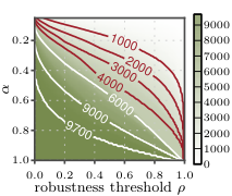
In order to evaluate if this holds for more datasets, we computed the number of free/non-derivable/totally shattered using different $\alpha$ s and normalized this by the number of robust itemsets exceeding the minimal robustness threshold of $0.1$ . In order to minimize the variance of behavior of the robustness in a single dataset, we consider an average over all test datasets, which we give in Figure 2. We see the same phenomenon as in Figure 1. Large values of $\alpha$ induce a skewed distribution which becomes more balanced as we decrease the value of $\alpha$ . Consider $\alpha=0.9$ . Our test datasets typically contain a lot of itemsets having only one transaction keeping them from becoming non-free. This can be seen as a dip of the curve for $\alpha=0.9$ at $\rho=0.9$ in Figure 2(a). A second dip at $\rho=0.81$ represents the itemsets that can be made non-free by deleting two transactions. As we make $\alpha$ smaller, these dips become less prominent.

(a) free itemsets

(b) totally shattered itemsets

2(c)

Figure 2: Average of the number of free/totally shattered/non-derivable itemsets as a function of

\rho

normalized by the number of itemsets for

\rho=0.1

. Average is taken over all test datasets

Based on this we chose $\alpha=0.5$ and plotted the number of free itemsets as a function of $\rho$ . Figure 3(a) shows that for the Zoo dataset there are many free itemsets with very different robustness values showing a rich structure that can be exploited to rank and reduce the number of itemsets. Similar results were observed for many of the UCI datasets. Figure 3(b) shows a representative example for the text datasets. While the distribution is much more skewed, a large $\rho$ would also reduce the number of itemsets by about 50%. Finally, Figure 3(c) shows an example for a large transactional dataset with 88k transactions. Using $\alpha=0.5$ generated a distribution where all values were close to one so we needed to set $\alpha=0.01$ to better show the quantitative differences of the itemsets. This demonstrates that the more transactions a dataset contains, the more skewed the distribution for a fixed $\alpha$ will be.

(a) Zoo (

\alpha=0.5,\tau=0.01

)

(b) LA12 (

\alpha=0.5,\tau=0.05

)

\alpha=0.01,\tau=0.0080

)

Figure 3: Number of free itemsets as a function of

\rho

6.3 Effect of noise for robust closed itemsets

Our next experiment is to see how robust closed itemsets behave when a dataset is exposed to noise. Our expectation is that most robust itemsets will stay closed and be ranked higher while the ranking of the less robust itemsets will be more susceptible to noise.

In order to do this, we created from each dataset a synthetic dataset having the same dimensions by sampling from a distribution. The underlying distribution had the same margins as the original data but otherwise items were independent. We then mix the original data with the synthetic one, that is, an entry in a mixed dataset is an entry from the synthetic dataset with the probability $\eta$ , and is an entry from the original dataset with the probability $1-\eta$ . We tested two different noise levels $\eta=0.05$ and $\eta=0.1$ .

We mined approximately $10\,000$ frequent closed itemsets from each original dataset. If the dataset contained less than $10\,000$ itemsets, we set the threshold to one transaction. Using the same thresholds we mined closed itemsets from the mixed datasets. We sorted the itemsets using Algorithm 1.

Let $X$ be an itemset ranked $i$ th in the original data. Assume that $X$ is ranked $j$ th in the noisy data. We define compliance of $X$ by $1/({\left|i-j\right|}+1)$ . The compliance will be $1$ if $i=j$ and decreases to $0$ the longer is the distance. The reason for using this particular definition is that we can naturally set compliance to $0$ if $X$ is not found in the noisy data. The compliances for top- $100$ itemsets are given in Figure 4.

(a) noise

\eta=0.05

(b) noise

\eta=0.1

Figure 4: Rank compliance of an itemset in a noisy data as a function of robustness in the original data. High compliance value imply that adding noise had little effect on the rank of an itemset. Median and quartiles are computed over all datasets.

From the figures we see that compliance stay high for robust itemsets and drop as we move further down the original ranking. That is, the more robust an itemset is, the less prone to noise it is. Adding more noise to the data implies less compliance. For example, for noise level $\eta=0.05$ , top-60 itemsets had a compliance of 0.25 or higher in half of the datasets. This means that their rank changed only by $3$ . On the other hand for noise level $\eta=0.1$ , top-50 itemsets had a compliance of 0.1 or higher in half of the dataset, in other words, ranks changed by $9$ .

6.4 Ranking without $\alpha$

Our next experiment was to compare the parameter-free ranking described in Section 4 against the rankings based on quantitative robustness given specific values of $\alpha$ . We expect that rankings are similar for large $\alpha$ values and difference increase when we lower $\alpha$ . For comparison we used the number of discordant pairs to calculate a distance of the rankings similar to Kendall’s $\tau$ . A discordant pair is a pair of itemsets $(X,Y)$ such that the first method ranks $X$ higher than $Y$ and the second method ranks $Y$ higher than $X$ . We normalize the number of observed discordant pairs by $100b$ , where $b$ is the maximum number of discordant pairs. Hence, we obtain a value between $0$ and $100$ . If there are no ties in robustness, then $b=N(N-1)/2$ , where $N$ is the number of itemsets. However if ties are presented, that is, the robustness induces a bucket order, then $b=N(N-1)/2-\sum_{i=1}B_{i}(B_{i}-1)/2$ , where $B_{i}$ is the size of each bucket, set of itemsets having the same robustness. Values close to $0$ mean that rankings are in agreement.

Typical examples are given in Table 6.4 for the Mushroom and Zoo datasets, along with the averages taken over all datasets. Surprisingly, the ranking distance is extremely small even for small values of $\alpha$ showing that the parameter free approach produces rankings similar to rankings under most $\alpha$ . Starting at $\alpha=0.5$ for Mushroom and all $\alpha$ for Zoo only about 1% of pairs are discordant. We see that values increase as we lower $\alpha$ which is expected since the parameter-free approach is based on large $\alpha$ values.

\tbl

Distance between parameter-free rankings and rankings based on $\alpha$ for Mushroom and Zoo datasets. Low values imply that rankings agree. Value range is $0$ – $100$ . Mushroom $(\tau=0.05)$ Zoo $(\tau=0.01)$ All datasets $\alpha$ free ts nd free ts nd free ts nd $0.1$ $0.30$ $0.82$ $0.39$ $14.91$ $7.26$ $7.62$ $4.35$ $4.25$ $2.80$ $0.2$ $0.078$ $0.27$ $0.089$ $10.01$ $8.69$ $4.31$ $2.59$ $2.67$ $2.11$ $0.3$ $0.017$ $0.11$ $0.044$ $5.94$ $5.40$ $2.23$ $1.46$ $1.63$ $1.45$ $0.4$ $0.0016$ $0.050$ $0.015$ $2.84$ $2.77$ $1.84$ $0.69$ $1.03$ $0.91$ $0.5$ $0.000032$ $0.027$ $0.0022$ $1.12$ $1.31$ $1.11$ $0.26$ $0.56$ $0.52$ $0.6$ $0.0000050$ $0.016$ $0.0023$ $0.32$ $0.58$ $0.56$ $0.082$ $0.25$ $0.27$ $0.7$ $0$ $0.0020$ $0.0011$ $0.017$ $0.20$ $0.25$ $0.013$ $0.073$ $0.11$ $0.8$ $0$ $0.0022$ $0$ $0$ $0$ $0.013$ $0.000074$ $0.013$ $0.031$ $0.9$ $0$ $0$ $0$ $0$ $0$ $0$ $0$ $0.00049$ $0.0039$

6.5 Top-k closed and free itemsets

Closed itemsets are often used for tasks requiring interpretation of the itemsets, because as maximum elements of an equivalence class they offer the most detailed description. We studied the highest ranked closed itemsets for text datasets that are easily understood without domain knowledge. As an illustrative example, we used the re0 news dataset from which we mine $2493$ closed itemsets with minimum support $\tau=0.05$ . We ordered these itemsets using the estimation technique given in Section 5.2 and list the top 45 itemsets in Table 6.5. The ranking is different from the one using support, less frequent (but more robust) itemsets are commonly ranked higher that frequent itemsets. For example, ’bank pct rate’ occurs before the much more frequent itemset ’bank pct’ showing that ’bank pct’ is only closed in the full dataset due to relatively few documents using it without also using ’rate’.

\tbl

Top-45 closed itemsets from re0 ( $\tau=0.05$ ) dataset. 1. pct 792 16. week 310 31. canada 117 2. bank 702 17. pct earlier 127 32. pct month 261 3. trade 485 18. japan 318 33. econom 295 4. billion 552 19. trade current 126 34. billion dlr mln 116 5. market 554 20. dlr 472 35. told bank 116 6. billion dlr 346 21. bank pct rate 287 36. told nation 116 7. offici 342 22. dollar 336 37. pct japan 115 8. mln 420 23. statem 122 38. pct adjust 115 9. nation 323 24. committe 121 39. billion current 115 10. rate 566 25. nation month 121 40. european 114 11. bank market 369 26. ministri 120 41. month japan 114 12. foreign 331 27. pct rise 269 42. bank ad market 114 13. pct figur 132 28. bank pct 407 43. action 114 14. pct rate 418 29. pct rate feb 119 44. trade world 114 15. month 391 30. lead 118 45. nation japan 114

Finally, we considered an alternative order by ranking itemsets based on how free they are. Note that a closed itemset is robust if the same transactions cannot be explained by a superset whereas a free itemset is robust if the same transactions cannot be explained by a subset. For example, a singleton $X$ will be ranked higher than singleton $Y$ if $X$ has lower support. The reason for this is that it requires less transactions to be removed in order to make $Y$ non-robust, namely the transactions not containing $Y$ . We present the top-45 free non-singleton itemsets from re0 news dataset in Table 6.5. These are frequent item pairs $ab$ such that $\mathit{sp}\mathopen{}\left(ab\right)\ll\mathit{sp}\mathopen{}\left(a\right)$ and $\mathit{sp}\mathopen{}\left(ab\right)\ll\mathit{sp}\mathopen{}\left(b\right)$ , that is, a non-robust free item pair $ab$ would be such that if we would remove a singleton $a$ (or $b$ ), then roughly the same transactions will still cover the pattern. An example of such non-robust free itemset is bank assist. This itemset is ranked as 2 465 out of 2 558 itemsets. The support of this itemset is 96 but the support of assist is 98, consequently there are only two documents in which assist occurs but not bank.

\tbl

Top-45 free non-singleton itemsets from re0 ( $\tau=0.05$ ) dataset. $1.$ billion rate $165$ $16.$ bank billion $287$ $31.$ govern dollar $92$ $2.$ rate dlr $132$ $17.$ billion pct $288$ $32.$ foreign februari $87$ $3.$ trade rate $146$ $18.$ rise dlr $118$ $33.$ januari dlr $81$ $4.$ trade bank $154$ $19.$ pct dlr $210$ $34.$ monei dlr $81$ $5.$ billion market $228$ $20.$ trade billion $223$ $35.$ dollar februari $89$ $6.$ rate mln $109$ $21.$ bank dlr $211$ $36.$ rise japan $78$ $7.$ trade pct $176$ $22.$ govern februari $77$ $37.$ februari japan $78$ $8.$ bank pct $407$ $23.$ govern mln $90$ $38.$ dollar offici $96$ $9.$ market rate $262$ $24.$ month dlr $141$ $39.$ rise offici $104$ $10.$ trade mln $130$ $25.$ trade dlr $222$ $40.$ pct mln $184$ $11.$ market dlr $186$ $26.$ pct market $306$ $41.$ februari dlr $94$ $12.$ month mln $106$ $27.$ market rise $133$ $42.$ foreign mln $95$ $13.$ trade market $203$ $28.$ februari offici $83$ $43.$ nation februari $89$ $14.$ rise mln $109$ $29.$ govern monei $77$ $44.$ januari mln $90$ $15.$ trade rise $115$ $30.$ januari govern $77$ $45.$ monei month $90$

7 Discussion

The experiments have shown that the number of itemsets can be largely reduced on many datasets when requiring a certain robustness. The fact that the results vary by dataset are another indication of the well known fact that itemset data with different structures (dense vs. sparse, many items vs. many transactions) behave very differently in mining tasks.

We believe that robust itemsets can be beneficial for post-processing techniques such as [6] or [32] that use itemsets as their input and remove redundancy in the pattern set. Robust itemsets can be used as an alternative input reducing their runtime without sacrificing performance. Also, robust itemsets could be used instead of closed-itemsets as seeds to the AC-Close algorithm for approximate itemset mining [11] improving its efficiency that was criticized in [19].

The ranking of itemsets by robustness presents a new interestingness measure that can be used to choose the top- $k$ itemsets for interpretation or other data mining tasks. The intuition of robustness should be easy to understand for analysts but which ranking is better for specific data mining tasks remains to be studied.

In particular it will be interesting to evaluate performance as features for classification tasks in contrast to direct mining of prediction tasks. For interpretable classifiers one would want itemsets to be long, thus use closed patterns. On the other hand the desire is for an itemset to be present in unseen data with high likelihood, so free itemset as the minimal elements of an equivalence class may generalize better. For both patterns we can ensure that they are present in many subsets of the training without actually sampling, potentially alleviating the need for nested cross validation.

8 Summary

We have shown how robustness under subsampling for common classes of itemsets can be computed efficiently without actually sampling the data. The experimental results show that the number of reported itemsets can be largely reduced on many datasets, in other words spurious itemsets that would not have been found in many subsets of the data are removed. The approach can further be used to rank itemsets for top- $k$ mining by robustness. Future work will investigate the effect of using robust itemsets on data mining tasks such as clustering, classification, and rule generation using itemsets.

References

Agrawal et al. (1993) Agrawal, R., Imielinski, T., and Swami, A. N. 1993. Mining association rules between sets of items in large databases. In SIGMOD. 207–216.
Asuncion and Newman (2007) Asuncion, A. and Newman, D. 2007. UCI machine learning repository.
Boulicaut et al. (2000) Boulicaut, J.-F., Bykowski, A., and Rigotti, C. 2000. Approximation of frequency queries by means of free-sets. In PKDD. 75–85.
Boulicaut et al. (2003) Boulicaut, J.-F., Bykowski, A., and Rigotti, C. 2003. Free-sets: A condensed representation of boolean data for the approximation of frequency queries. DMKD 7, 1, 5–22.
Brin et al. (1997) Brin, S., Motwani, R., and Silverstein, C. 1997. Beyond market baskets: Generalizing association rules to correlations. In SIGMOD. 265–276.
Bringmann and Zimmermann (2009) Bringmann, B. and Zimmermann, A. 2009. One in a million: picking the right patterns. KAIS 18, 1, 61–81.
Calders and Goethals (2007) Calders, T. and Goethals, B. 2007. Non-derivable itemset mining. DMKD 14, 1, 171–206.
Calders et al. (2007) Calders, T., Goethals, B., and Mampaey, M. 2007. Mining itemsets in the presence of missing values. In SAC. 404–408.
Calders et al. (2006) Calders, T., Rigotti, C., and Boulicaut, J.-F. 2006. A survey on condensed representations for frequent sets. In Constraint-Based Mining and Inductive Databases. 64–80.
Cheng et al. (2007) Cheng, H., Yan, X., Han, J., and Hsu, C. 2007. Discriminative frequent pattern analysis for effective classification. In ICDE. 716–725.
Cheng et al. (2006) Cheng, H., Yu, P. S., and Han, J. 2006. AC-Close: Efficiently mining approximate closed itemsets by core pattern recovery. In ICDM. IEEE, 839–844.
Coenen (2003) Coenen, F. 2003. The LUCS-KDD discretised/normalised ARM and CARM data library.
De Bie (2011) De Bie, T. 2011. Maximum entropy models and subjective interestingness: an application to tiles in binary databases. 1–40.
Gallo et al. (2007) Gallo, A., De Bie, T., and Cristianini, N. 2007. Mini: Mining informative non-redundant itemsets. In ECMLPKDD. 438–445.
Geerts et al. (2004) Geerts, F., Goethals, B., and Mielikäinen, T. 2004. Tiling databases. In Proc. Discovery Science. 278–289.
Ghoshal and Barabási (2011) Ghoshal, G. and Barabási, A.-L. 2011. Ranking stability and super-stable nodes in complex networks. Nature Communications 2.
Gionis et al. (2007) Gionis, A., Mannila, H., Mielikäinen, T., and Tsaparas, P. 2007. Assessing data mining results via swap randomization. TKDD 1, 3.
Goethals and Zaki (2003) Goethals, B. and Zaki, M. 2003. FIMI ’03, frequent itemset mining implementations. In ICDM 2003 Workshop, FIMI.
Gupta et al. (2008) Gupta, R., Fang, G., Field, B., Steinbach, M., and Kumar, V. 2008. Quantitative evaluation of approximate frequent pattern mining algorithms. In KDD. 301–309.
Hanhijärvi et al. (2009) Hanhijärvi, S., Ojala, M., Vuokko, N., Puolamäki, K., Tatti, N., and Mannila, H. 2009. Tell me something I don’t know: randomization strategies for iterative data mining. In Proceedings of the 15th ACM SIGKDD International Conference on Knowledge Discovery and Data Mining (KDD 2009). 379–388.
Hipp et al. (2000) Hipp, J., Güntzer, U., and Nakhaeizadeh, G. 2000. Algorithms for association rule mining - a general survey and comparison. SIGKDD Explorations 2, 1, 58–64.
Luccese et al. (2010) Luccese, C., Orlando, S., and Perego, R.Casas-Garriga, G. 2010. Mining top-k patterns from binary datasets in presence of noise. In ICDM.
Mielikäinen (2005) Mielikäinen, T. 2005. Transaction databases, frequent itemsets, and their condensed representations. In KDID. 139–164.
Misra et al. (2012) Misra, G., Golshan, B., and Terzi, E. 2012. A framework for evaluating the smoothness of data-mining results. In ECMLPKDD 2012. 660–675.
Moerchen et al. (2010) Moerchen, F., Thies, M., and Ultsch, A. 2010. Efficient mining of all margin-closed itemsets with applications in temporal knowledge discovery and classification by compression. KAIS.
Pasquier et al. (1999) Pasquier, N., Bastide, Y., Taouil, R., and Lakhal, L. 1999. Discovering frequent closed itemsets for association rules. In ICDT. 398–416.
Pei et al. (2001) Pei, J., Han, J., and Lakshmanan, L. V. S. 2001. Mining frequent itemsets with convertible constraints. In ICDE. 433–442.
Smets and Vreeken (2011) Smets, K. and Vreeken, J. 2011. The odd one out: Identifying and characterising anomalies. In SDM.
Tatti (2008) Tatti, N. 2008. Maximum entropy based significance of itemsets. KAIS 17, 1, 57–77.
Tatti and Moerchen (2011) Tatti, N. and Moerchen, F. 2011. Finding robust itemsets under subsampling. In 11th IEEE International Conference on Data Mining, ICDM 2011. 705–714.
Uno and Arimura (2007) Uno, T. and Arimura, H. 2007. An efficient polynomial delay algorithm for pseudo frequent itemset mining. In Discovery Science. Springer, 219–230.
Vreeken et al. (2011) Vreeken, J., van Leeuwen, M., and Siebes, A. 2011. Krimp: mining itemsets that compress. DMKD 23, 1, 169–214.
Wang et al. (1999) Wang, K., Xu, C., and Liu, B. 1999. Clustering transactions using large items. In CIKM. 483–490.
Webb (2007) Webb, G. I. 2007. Discovering significant patterns. Mach. Learn. 68, 1, 1–33.
Xin et al. (2005) Xin, D., Han, J., Yan, X., and Cheng, H. 2005. Mining compressed frequent-pattern sets. In VLDB. 709–720.
Zhao and Karypis (2002) Zhao, Y. and Karypis, G. 2002. Evaluation of hierarchical clustering algorithms for document datasets. In CIKM. 515–524.

Finding Robust Itemsets Under Subsampling

Abstract

Keywords:

category

keywords

1 Introduction

2 Related work and motivation

3 Robust itemsets

3.1 Notation and definitions

Example 3.1.

Closed Itemsets

Free Itemsets

Example 3.2.

Non-derivable Itemsets

Example 3.3.

3.2 Measuring robustness

Definition 3.4.

Definition 3.5.

Example 3.6.

Proposition 3.7.

Proof 3.8.

Definition 3.9.

Proposition 3.10.

Proof 3.11.

Proposition 3.12.

Lemma 3.13.

Proof 3.14.

Proof 3.15 (of Proposition 3.12).

Example 3.16.

3.3 Computing the measure

Proposition 3.17.

Proof 3.18.

Proposition 3.19.

Proof 3.20.

Proposition 3.21.

Proof 3.22.

Proposition 3.23.

Proof 3.24.

Example 3.25.

Proposition 3.26.

Proof 3.27.

Lemma 3.28.

Proof 3.29.

Lemma 3.30.

Proof 3.31.

4 Ordering patterns

4.1 Measuring robustness when α\alpha approaches 11

Proposition 4.1.

Proof 4.2.

Definition 4.3.

4.2 Properties of the order

Lemma 4.4.

Proposition 4.5.

Proof 4.6.

Definition 4.7.

Proposition 4.8.

Proof 4.9.

Free itemsets

Closed itemsets

Totally shattered itemsets

Non-derivable itemsets

Example 4.10.

Lemma 4.11.

Proof 4.12.

Proposition 4.13.

Proof 4.14.

5 Computing order in practice

5.1 Free and totally shattered itemsets

Definition 5.1.

Proposition 5.2.

Proof 5.3.

Definition 5.4.

Corollary 5.5.

Corollary 5.6.

Example 5.7.

Definition 5.8.

Proposition 5.9.

Proposition 5.10.

Proposition 5.11.

Proof 5.12.

4.1 Measuring robustness when $\alpha$ approaches $1$

6.4 Ranking without $\alpha$