A gauge invariant prescription to avoid $\gamma$-crossing instability in Galileon bounce

The most investigated alternative to the inflationary paradigm is the classical non-singular bouncing scenario. In a non-singular bouncing scenario, the universe undergoes a period of contraction until the scale factor attains a minimum value and thereafter it transits to the phase of expansion. The Hubble parameter is negative during the contraction, and it is positive during the expansion. These two phases are connected by a bouncing phase where the rate of change of the Hubble parameter is positive. In Einsteinian gravity this phase is obtained by violating the null energy condition (NEC). During this NEC violating phase, the Hubble parameter grows and reaches zero and continues to grow until it reaches a positive value and then it begins to decrease. It is well known that a canonical scalar field with quadratic kinetic term does not violate the NEC. To achieve this condition, various models have been considered Brandenberger and Peter 2016. One of the best motivated model is the cubic Galileon bounce Qiu et al. 2011; Easson et al. 2011; Brandenberger and Peter 2016; Akama and Kobayashi 2017; Cai et al. 2017.

It has been recognized that in the Galileon bounce models, there is a crossing point viz. $\gamma$-crossing, where the equation of motion governing the perturbation becomes numerically unstable Battarra et al. 2014; Ijjas 2018; Ijjas and Steinhardt 2016. It is also understood that this is not a real divergence in the perturbation. Usually, this instability can be evaded by choosing a particular gauge such as harmonic gauge or Newtonian gauge to evolve the perturbations Battarra et al. 2014; Ijjas 2018; Mironov et al. 2018. In this work, we demonstrate that the primordial perturbations can be evolved across the $\gamma$-crossing by solving two first order differential equations governing suitable gauge invariant quantities.

We shall work with natural units such that $\hbar=c=1$, and set the Planck mass to be $M_{{}_{\rm Pl}}=\left(8\,\pi\,G\right)^{-1/2}$. We shall adopt the metric signature of $\left(-,+,+,+\right)$. Note that, while Greek indices shall denote the spacetime coordinates, the Latin indices shall represent the spatial coordinates, except for $k$ which shall be reserved for denoting the wavenumber. Moreover, an overdot and an overprime shall denote differentiation with respect to the cosmic and the conformal time coordinates, respectively.

This paper is organized as follows. In the following section, we shall briefly discuss the Galileon bounce. In section III, we shall obtain the relevant first order equations governing the perturbations. In section IV, we shall use these equations to evolve the scalar perturbations in a particular bouncing scenario called matter bounce. We shall conclude in section V with brief summary and outlook.

We assume that the bounce stage is driven by a single scalar field $\phi$ that is described by the generalized cubic Galileon action Brandenberger and Peter 2016; Qiu et al. 2011; Easson et al. 2011; Ijjas and Steinhardt 2016

$$S=\int{\rm d}^{4}\,x\,\sqrt{-g}\,\cal{L},$$

(1)

with the Lagrangian density

$${\cal L}=K\left(X,\phi\right)-b(\phi)X\Box\phi,$$

(2)

where

$$X=-\frac{1}{2}\,{\partial}_{\mu}\phi\,{\partial}^{\mu}\phi,$$

(3)

and $b(\phi)$ is the dimensionless coupling of the scalar field $\phi$ to the Galileon term. We shall consider the background to be the spatially flat, Friedmann-Lemaître-Robertson-Walker (FLRW) metric that is described by the line-element

$${\rm d}s^{2}=-{\rm d}t^{2}+a^{2}(t)\,\delta_{ij}\,{\rm d}x^{i}\,{\rm d}x^{j},$$

(4)

where $a(t)$ is the scale factor. Varying the action (1) with respect to the background metric we get the Friedmann equations in terms of the background quantities as

	$\displaystyle 3\,M_{{}_{\rm Pl}}^{2}\,H^{2}$	$\displaystyle=$	$\displaystyle-K\,+K_{X}\,\dot{\phi}^{2}-\frac{1}{2}\,b_{\phi}\,\dot{\phi}^{4}+3\,H\,b\,\dot{\phi}^{3},\quad$		(5a)
	$\displaystyle-2M_{{}_{\rm Pl}}^{2}\dot{H}$	$\displaystyle=$	$\displaystyle K_{X}\,\dot{\phi}^{2}-b_{\phi}\,\dot{\phi}^{4}+3\,H\,b\,\dot{\phi}^{3}-b\,\ddot{\phi}\,\dot{\phi}^{2},\quad$		(5b)

where subscripts $\phi$ and $X$ denote the differentiation with respect to $\phi$ and $X$ respectively. By choosing the functions $K(\phi,\chi)$ and $b(\phi)$ suitably, one can model the early contracting phase, the NEC violating phase and the expanding phase of the universe Brandenberger and Peter 2016; Qiu et al. 2011; Easson et al. 2011; Ijjas and Steinhardt 2016.

If we take into account the scalar perturbations to the background metric (4), then the FLRW line-element, in general, can be written as Mukhanov et al. 1992

$${\rm d}s^{2}=-\left(1+2\,A\right)\,{\rm d}t^{2}+2\,a(t)\,(\partial_{i}B)\;{\rm d}t\;{\rm d}x^{i}\,+a^{2}(t)\;\left[(1-2\,\psi)\;\delta_{ij}+2\,\left(\partial_{i}\,\partial_{j}E\right)\right]\,{\rm d}x^{i}\,{\rm d}x^{j},$$

(6)

where $A$, $B$, $\psi$ and $E$ are four scalar functions that describe the perturbations, which depend on time as well as space.

In order to identify the suitable gauge invariant quantities to evolve the perturbations, it is important to understand how each of the basic perturbations, $A$, $B$, $\psi$, $E$ and $\delta\phi$, transform under the coordinate transformations. It is easy to show that, under the coordinate transformations

$$t\to t+\delta t,\quad x_{i}\to x_{i}+{\partial}_{i}\delta x,$$

(7)

the functions $A$, $B$, $\psi$ and $E$ transform as follows:

	$\displaystyle A$		$\displaystyle\to A-\dot{\delta t},$		(8a)
	$\displaystyle B$		$\displaystyle\to B+\left(\delta t/a\right)-a\,\dot{\delta x},$		(8b)
	$\displaystyle\psi$		$\displaystyle\to\psi+H\,\delta t,$		(8c)
	$\displaystyle E$		$\displaystyle\to E-\delta x.$		(8d)

It is evident from the expression (8c) that the spatially flat gauge, wherein $\psi=0$, is ill-defined at the bounce where $H=0$. It is convenient to define $\sigma=a\,B-a^{2}\,\dot{E}$ and this quantity transforms as

$$\sigma\to\sigma+\delta t.$$

(9)

The perturbation in the scalar field transforms as

$$\delta\phi\to\delta\phi-\dot{\phi}\,\delta t.$$

(10)

Using the above information, we can define the following three gauge invariant quantities as

	$\displaystyle{\mathcal{R}}$	$\displaystyle=$	$\displaystyle\psi+H\,\frac{\delta\phi}{\dot{\phi}},$		(11a)
	$\displaystyle\Sigma$	$\displaystyle=$	$\displaystyle\sigma+\frac{\delta\phi}{\dot{\phi}},$		(11b)
	$\displaystyle\mathcal{A}$	$\displaystyle=$	$\displaystyle A-\left(\frac{\delta\phi}{\dot{\phi}}\right)^{\cdot}.$		(11c)

At the first order in the perturbations, three of the Einstein’s equations of our interest are given by Mukhanov et al. 1992; Sriramkumar 2009

	$\displaystyle 3\,H\,\left(H\,A+\dot{\psi}\right)-\frac{\nabla^{2}}{a^{2}}\left[\psi-H\,\sigma\right]$	$\displaystyle=$	$\displaystyle-\frac{\delta T^{0}_{0}}{2\,M_{{}_{\rm Pl}}^{2}},$		(12a)
	$\displaystyle{\partial}_{i}\left(H\,A+\dot{\psi}\right)$	$\displaystyle=$	$\displaystyle-\frac{\delta T^{0}_{i}}{2\,M_{{}_{\rm Pl}}^{2}},$		(12b)
	$\displaystyle A-\psi+\frac{1}{a}\,\left(a\,\sigma\right)^{\cdot}$	$\displaystyle=$	$\displaystyle 0,$		(12c)

where $\delta T^{\mu}_{\nu}$ is the perturbed stress-energy tensor associated with the Galileon. The equation (12c) follows from the fact that there are no anisotropic stresses present. The components of $\delta T^{\mu}_{\nu}$ can be calculated from the action (1) to be

	$\displaystyle\frac{\delta T^{0}_{0}}{2\,M_{{}_{\rm Pl}}^{2}}$	$\displaystyle=$	$\displaystyle-\bigg[\left(\theta+3\,H^{2}-3\,\gamma^{2}\right)A+\frac{1}{2}\,b\,\dot{\phi}^{3}\left(3\,\dot{\psi}+\frac{\nabla^{2}}{a^{2}}\,\sigma\right)$		(13a)
			$\displaystyle-\left(\theta+3\,H\,\gamma-3\,\gamma^{2}\right)\left(\frac{\delta\phi}{\dot{\phi}}\right)^{\cdot}-\left(3\,\dot{H}\,\gamma-\frac{\nabla^{2}}{2\,a^{2}}\,b\,\dot{\phi}^{3}\right)\frac{\delta\phi}{\dot{\phi}}\bigg],$
	$\displaystyle\frac{\delta T^{0}_{i}}{2\,M_{{}_{\rm Pl}}^{2}}$	$\displaystyle=$	$\displaystyle-\partial_{i}\left[\frac{1}{2}\,b\,\dot{\phi}^{3}\,A-\left(H-\gamma\right)\left(\frac{\delta\phi}{\dot{\phi}}\right)^{\cdot}-\dot{H}\,\frac{\delta\phi}{\dot{\phi}}\right],$		(13b)

where

	$\displaystyle\gamma$	$\displaystyle=$	$\displaystyle H-\frac{1}{2}\,b\,\dot{\phi}^{3},$		(14a)
	$\displaystyle\theta$	$\displaystyle=$	$\displaystyle 3\left(\gamma-H\right)^{2}-\dot{H}+\frac{1}{2}\,b\,\ddot{\phi}\,\dot{\phi}^{2}+\frac{1}{2}\,K_{XX}\dot{\phi}^{4}+\frac{3}{2}\,b\,H\,\dot{\phi}^{3}-\frac{1}{2}\,b_{\phi}\dot{\phi}^{4}.$		(14b)

We define $\delta T^{0}_{i}=-\partial_{i}\delta q$ and the quantity $\delta q$ transforms under coordinate transformations (7) as

$$\delta q\to\delta q+2\,\dot{H}\delta t.$$

(15)

It is important to note that the comoving gauge, where $\delta q=0$, is ill-defined at $\dot{H}=0$.

The scalar part of the linearized Einstein equations (12) can be rewritten in terms of the gauge invariant quantities defined in equations (11a), (11b) and (11c) as

	$\displaystyle{\mathcal{R}}^{\prime}+\frac{k^{2}\,\gamma}{a\,\theta}\,\left({\mathcal{R}}-\gamma\,\Sigma\right)$	$\displaystyle=$	$\displaystyle 0,$		(16a)
	$\displaystyle{\mathcal{R}}^{\prime}+a\,\gamma\,\mathcal{A}$	$\displaystyle=$	$\displaystyle 0,$		(16b)
	$\displaystyle\Sigma^{\prime}+a\,H\,\Sigma+\frac{k^{2}}{a\,\theta}\,\left({\mathcal{R}}-\gamma\,\Sigma\right)-a\,{\mathcal{R}}$	$\displaystyle=$	$\displaystyle 0.$		(16c)

Note that the above equations are written in terms of conformal time coordinate. From equations (16a) and (16b), it is evident that ${\mathcal{R}}^{\prime}=0$ at $\gamma=0$. One can easily obtain the second order differential equation governing ${\mathcal{R}}$ from equations (16a) and (16c) as

$${\mathcal{R}}^{\prime\prime}+2\,\frac{z^{\prime}}{z}\,{\mathcal{R}}^{\prime}+k^{2}\,c_{s}^{2}\,{\mathcal{R}}=0,$$

(17)

where,

	$\displaystyle z^{2}$	$\displaystyle=$	$\displaystyle 2\,a^{2}\frac{\theta}{\gamma^{2}},$		(18)
	$\displaystyle c_{s}^{2}$	$\displaystyle=$	$\displaystyle\frac{\gamma^{2}}{\theta}\,\left(\frac{H}{\gamma}-\frac{\gamma^{\prime}}{a\,\gamma^{2}}-1\right).$		(19)

It should be mentioned that the quantity $\theta$ requires to be positive to avoid the quantum ghost instabilities Lehners 2008; Ijjas and Steinhardt 2016. It is evident from the above expressions that, the coefficient of ${\mathcal{R}}^{\prime}$

$$2\,\frac{z^{\prime}}{z}=2\,a\,H+\frac{\theta^{\prime}}{\theta}-2\,\frac{\gamma^{\prime}}{\gamma},$$

(20)

diverges at $\gamma=0$. This is not a concern, since, as we have argued earlier, ${\mathcal{R}}^{\prime}$ becomes zero at this point. In other words, from equations (16a) and (16b), it is evident that the ratio ${\mathcal{R}}^{\prime}/\gamma$ is finite. This implies that there is no divergence in ${\mathcal{R}}$ at $\gamma$-crossing. However, the equation (17) can be numerically unstable around $\gamma=0$ (for a discussion on this point, see Refs. Battarra et al. 2014; Ijjas 2018; Ijjas and Steinhardt 2016). In order to avoid this stiffness in the equation one can use equations (16a) and (16c) for evolving the perturbations. In the following section, we shall illustrate this point with a specific example.

In order to show that the quantity ${\mathcal{R}}$ evolves smoothly across the point where $\gamma=0$ without any divergence, we solve the equations (16a) and (16c) for a bounce model called the matter bounce. Matter bounce is a popular alternative to inflation due to the fact that it generates scale invariant perturbations as in the case of inflation Battefeld and Peter 2015; Brandenberger 2012. In matter bounce scenarios, during the early stages of the contracting phase, the scale factor behaves as in a matter dominated universe. In this work, we choose to work with a scale factor of the form Raveendran et al. 2018

$$a(\eta)=a_{0}\left(1+k_{0}^{2}\,\eta^{2}\right),$$

(21)

where $a_{0}$ is the value of the scale factor at the bounce and $k_{0}$ is the scale associated with the bounce. The above scale factor describes the evolution of matter dominated contracting phase, the bounce phase and the expanding phase up to the beginning of radiation dominated epoch. Using this scale factor the Hubble parameter and its time derivative can be calculated in terms of scale factor as

	$\displaystyle H^{2}=\left(\frac{2k_{0}}{a_{0}}\right)^{2}\left[\frac{1}{(a/a_{0})^{3}}-\frac{1}{(a/a_{0})^{4}}\right],$		(22a)
	$\displaystyle\dot{H}=-\left(\frac{k_{0}}{a_{0}}\right)^{2}\left[\frac{6}{(a/a_{0})^{3}}-\frac{8}{(a/a_{0})^{4}}\right].$		(22b)

We consider the conventional form of Galileon action with

$$K(X,\phi)=\alpha(\phi)\,X+\beta(\phi)\,X^{2}-V(\phi),$$

(23)

where $\alpha({\phi})$ and $\beta({\phi})$ are functions of $\phi$ and $V(\phi)$ is the scalar potential Easson et al. 2011. For simplicity, we assume

$$\dot{\phi}^{2}=\left(\frac{c_{0}k_{0}}{a_{0}}\right)^{2}\frac{1}{(a/a_{0})^{3}},$$

(24)

where $c_{0}$ is a constant. We also set $V(\phi)=0$ and $b$ to be a constant as $b=b_{0}/(c_{0}^{3}\,a_{0}^{2}\,\,k_{0}^{2})$. Upon using equations (14), (21) and (24), one can obtain

	$\displaystyle\gamma$	$\displaystyle=$	$\displaystyle\frac{a_{0}\,k_{0}}{a^{2}}\,\left(2\,k_{0}\,\eta-\frac{b_{0}}{2\,a^{5/2}\,a_{0}^{3/2}}\right),$		(25a)
	$\displaystyle\theta$	$\displaystyle=$	$\displaystyle\frac{3\,a_{0}^{2}\,k_{0}^{2}}{4\,a^{4}}\bigg[\left(3\,k_{0}\,\eta-\frac{b_{0}}{a^{5/2}\,a_{0}^{3/2}}\right)^{2}+8+31\,k_{0}^{2}\,\eta^{2}\bigg].$		(25b)

The evolution of $\gamma$ around the $\gamma$-crossing in our model of interest is shown in the figure 1. It is clear from the expression (25b) that in our model, $\theta$ is always positive and hence there is no appearance of ghost instability.

Let us now integrate the equations (16a) and (16c) numerically by using the analytical expressions for the background quantities $\gamma$ and $\theta$. The initial conditions of ${\mathcal{R}}$ can be obtained from the Bunch-Davies initial condition as

$${\mathcal{R}}_{i}=\frac{1}{z\,\sqrt{2\,c_{s}\,k}}\,{\rm e}^{-i\,c_{s}\,k\,\eta}.$$

(26)

Similarly the initial condition for the quantity $\Sigma$ can be obtained from the relation (16a).

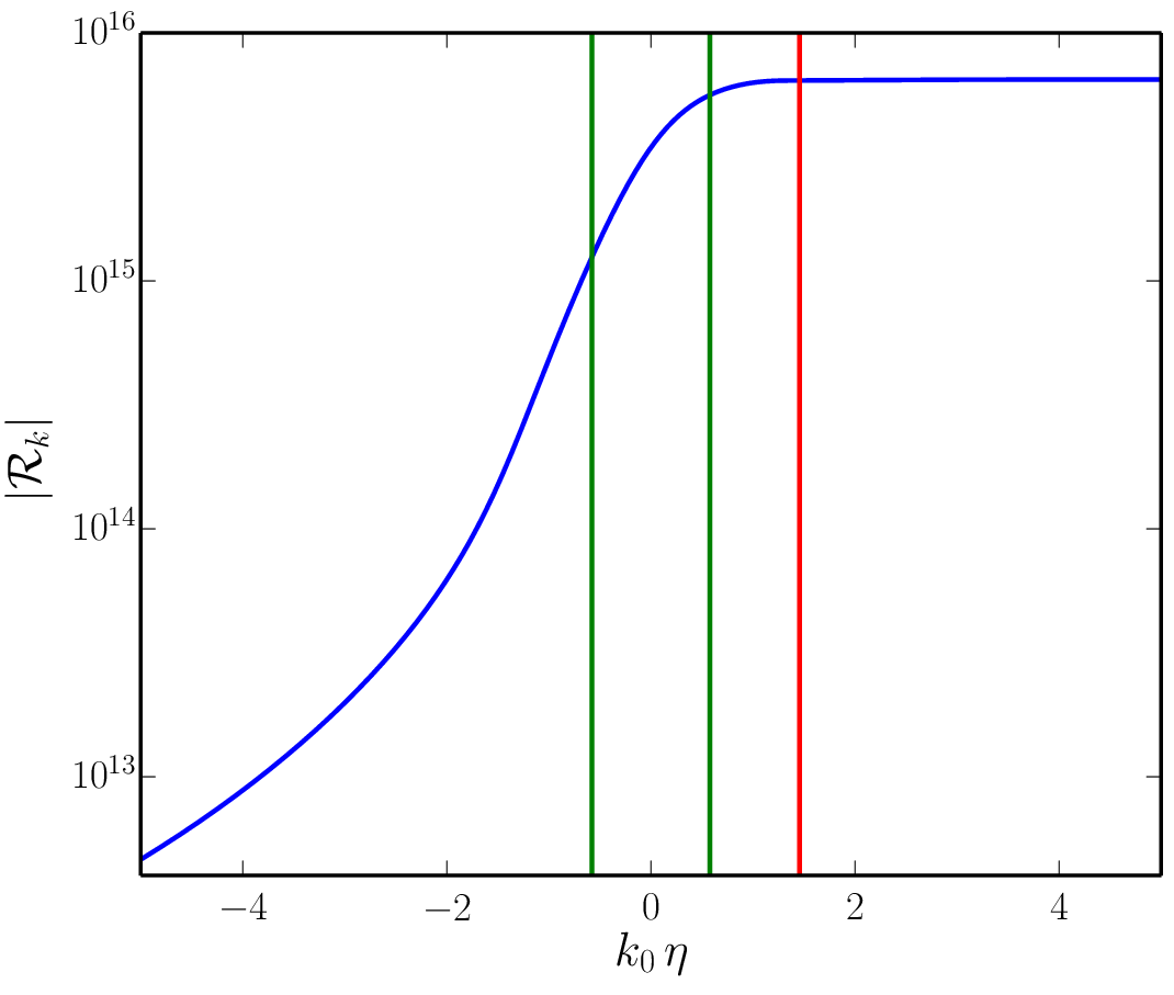
The figure 2 shows the evolution of the quantity ${\mathcal{R}}$ which is obtained by integrating the equations (16a) and (16c). It is clear from the figure that the quantity ${\mathcal{R}}$ evolves smoothly across the point where $\gamma=0$ ($\gamma$-crossing). The evolution of $\Sigma$ is shown in figure 3.

In this work we have found that the commonly used gauges, such as spatially flat and comoving gauges, cannot be used for studying the evolution of the perturbations in bouncing scenarios. More specifically, while the spatially flat gauge is ill-defined at the bounce, the comoving gauge is ill-defined at $\dot{H}=0$.

For studying the evolution of perturbations in the Galileon bounce, the usual practice is to use a gauge in which the equation governing the perturbation does not show any divergence at $\gamma$-crossing. In this work, we have demonstrated that the gauge invariant perturbation ${\mathcal{R}}$, defined in the equation (11a), can be used to evolve the perturbation in Galileon bounce. Moreover, we have also shown that, in order to avoid the numerical instability near the $\gamma$-crossing, one can solve the first order equations (16) for studying the evolution of ${\mathcal{R}}$. We have explicitly illustrated this point in a matter bounce model which is described by the scale factor of the form (21).

We believe that we can extend this method of evolving the perturbations across the $\gamma$-crossing using the first order equations in models derived from more general Horndesky theories Ijjas 2018. We are presently investigating this possibility.

References

- Brandenberger and Peter (2016) R. Brandenberger and P. Peter, Bouncing Cosmologies: Progress and Problems, (2016), arXiv:1603.05834 [hep-th] .
- Qiu et al. (2011) T. Qiu, J. Evslin, Y.-F. Cai, M. Li, and X. Zhang, Bouncing Galileon Cosmologies, JCAP 1110, 036, arXiv:1108.0593 [hep-th] .
- Easson et al. (2011) D. A. Easson, I. Sawicki, and A. Vikman, G-Bounce, JCAP 1111, 021, arXiv:1109.1047 [hep-th] .
- Akama and Kobayashi (2017) S. Akama and T. Kobayashi, Generalized multi-Galileons, covariantized new terms, and the no-go theorem for nonsingular cosmologies, Phys. Rev. D95, 064011 (2017), arXiv:1701.02926 [hep-th] .
- Cai et al. (2017) Y. Cai, H.-G. Li, T. Qiu, and Y.-S. Piao, The Effective Field Theory of nonsingular cosmology: II, Eur. Phys. J. C77, 369 (2017), arXiv:1701.04330 [gr-qc] .
- Battarra et al. (2014) L. Battarra, M. Koehn, J.-L. Lehners, and B. A. Ovrut, Cosmological Perturbations Through a Non-Singular Ghost-Condensate/Galileon Bounce, JCAP 1407, 007, arXiv:1404.5067 [hep-th] .
- Ijjas (2018) A. Ijjas, Space-time slicing in Horndeski theories and its implications for non-singular bouncing solutions, JCAP 1802 (02), 007, arXiv:1710.05990 [gr-qc] .
- Ijjas and Steinhardt (2016) A. Ijjas and P. J. Steinhardt, Classically stable nonsingular cosmological bounces, Phys. Rev. Lett. 117, 121304 (2016), arXiv:1606.08880 [gr-qc] .
- Mironov et al. (2018) S. Mironov, V. Rubakov, and V. Volkova, Bounce beyond Horndeski with GR asymptotics and -crossing, JCAP 1810 (10), 050, arXiv:1807.08361 [hep-th] .
- Mukhanov et al. (1992) V. F. Mukhanov, H. A. Feldman, and R. H. Brandenberger, Theory of cosmological perturbations, Physics Reports 215, 203 (1992).
- Sriramkumar (2009) L. Sriramkumar, An introduction to inflation and cosmological perturbation theory, (2009), arXiv:0904.4584 [astro-ph.CO] .
- Lehners (2008) J.-L. Lehners, Ekpyrotic and Cyclic Cosmology, Phys. Rept. 465, 223 (2008), arXiv:0806.1245 [astro-ph] .
- Battefeld and Peter (2015) D. Battefeld and P. Peter, A Critical Review of Classical Bouncing Cosmologies, Phys.Rept. 571, 1 (2015), arXiv:1406.2790 [astro-ph.CO] .
- Brandenberger (2012) R. H. Brandenberger, The Matter Bounce Alternative to Inflationary Cosmology, (2012), arXiv:1206.4196 [astro-ph.CO] .
- Raveendran et al. (2018) R. N. Raveendran, D. Chowdhury, and L. Sriramkumar, Viable tensor-to-scalar ratio in a symmetric matter bounce, JCAP 1801 (01), 030, arXiv:1703.10061 [gr-qc] .