Manifold interpolation and model reduction
Abstract
One approach to parametric and adaptive model reduction is via the interpolation of orthogonal bases, subspaces or positive definite system matrices. In all these cases, the sampled inputs stem from matrix sets that feature a geometric structure and thus form so-called matrix manifolds. This work will be featured as a chapter in the upcoming Handbook on Model Order Reduction, (P. Benner, S. Grivet-Talocia, A. Quarteroni, G. Rozza, W. H. A. Schilders, L. M. Silveira, eds, to appear on DE GRUYTER) and reviews the numerical treatment of the most important matrix manifolds that arise in the context of model reduction. Moreover, the principal approaches to data interpolation and Taylor-like extrapolation on matrix manifolds are outlined and complemented by algorithms in pseudo-code.
keywords
parametric model reduction, matrix manifold, Riemannian computing, geodesic interpolation, interpolation on manifolds, Grassmann manifold, Stiefel manifold, matrix Lie groupAMS
15-01, 15A16, 15B10, 15B48, 53-04, 65F60, 41-01, 41A05, 65F99, 93A15, 93C301 Introduction & Motivation
This work addresses interpolation approaches for parametric model reduction. This includes techniques for
- •
computing trajectories of parameterized subspaces,
- •
computing trajectories of parameterized reduced orthogonal bases,
- •
structure-preserving interpolation.
Mathematically, this requires data processing on nonlinear matrix manifolds. The exposition at hand intends to be an introduction and a reference guide to numerical procedures with matrix manifold-valued data. As such it addresses practitioners and scientists new to the field. It covers the essentials of those matrix manifolds that arise most frequently in practical problems in model reduction. The main purpose is not to discuss concrete model reduction applications, but rather to provide the essential tools, building blocks and background theory to enable the reader to devise her/his own approaches for such applications.
The text was designed such that it works as a commented formula collection, meanwhile giving sufficient context, explanations and, not least, precise references to enable the interested reader to immerse further in the topic.
1.1 Parametric model reduction via manifold interpolation: An introductory example
The basic objective in model reduction is to emulate a large-scale dynamical system with very few degrees of freedom such that its input/output behavior is preserved as well as possible. While classical model reduction techniques aim at producing an accurate low-order approximation to the autonomous behavior of the original system, parametric model reduction (pMOR) tries to account for additional system parameters. If we look for instance at aircraft aerodynamics, an important task is to solve the unsteady Navier-Stokes equations at various flight conditions, which are, amongst others, specified by the altitude, the viscosity of the fluid (i.e. the Reynolds number) and the relative velocity (i.e. the Mach number).We explain the objective of pMOR with the aid of a generic example in the context of proper orthogonal decomposition-based model reduction. Similar considerations apply to frequency domain approaches, Krylov subspace methods and balanced truncation, which are discussed in other chapters of the upcoming Handbook on Model Order Reduction. Consider a spatio-temporal dynamical system in semi-discrete form
| (1) |
where is the spatially discretized state vector of dimension , the vector accounts for additional system parameters and is the (possibly nonlinear, parameter-dependent) right hand side function. Projection-based MOR starts with constructing a suitable low-dimensional subspace that acts as a space of candidate solutions.
Subspace construction. One way to construct the required projection subspace is the proper orthogonal decomposition (POD), [48].In its simplest form, the POD can be summarized as follows. For a fixed system parameter , let be a set of state vectors satisfying (1) and let . The state vectors are called snapshots and the matrix is called the associated snapshot matrix. POD is concerned with finding a subspace of dimension represented by a column-orthogonal matrix such that the error between the input snapshots and their orthogonal projection onto is minimized:
The main result of POD is that for any , the best -dimensional approximation of in the above sense is , where are the eigenvectors of the matrix corresponding to the largest eigenvalues. The subspace is called the POD subspace and the matrix is the POD basis matrix. The same subspace is obtained via a compact singular value decomposition (SVD) of the snapshot matrix , truncated to the first columns of by setting . For more details, see, e.g. [17, §3.3]. In the following, we drop the index and assume that is already the truncated matrix .
Since the input snapshots are supplied at a fixed system parameter vector , the POD subspace is considered to be an appropriate space of solution candidates at .
Projection. POD leads to a parameter decoupling
| (2) |
In this way, the time trajectory of the reduced model is uniquely defined by the coefficient vector that represents the reduced state vector with respect to the subspace . Given a matrix such that the matrix pair is bi-orthogonal, i.e. , the original system (1) can be reduced in dimension as follows. Substituting (2) in (1) and multiplying with from the left leads to
| (3) |
This approach goes by the name of Petrov-Galerkin projection, if and Galerkin projection if . There are various ways to proceed from (3) depending on the nature of the function and many of them are discussed in other chapters of the upcoming Handbook on Model Order Reduction. 11 1 If is linear, the reduced operator can be computed a priori (‘offline’) and stays fixed throughout the time integration. If is affine, the same approach can be carried over to the affine building blocks of , see e.g. [42]. For a nonlinear , an affine approximation can be constructed via the emperical interpolation method (EIM, [14]). Other approaches that address nonlinearities include the discrete empirical interpolation method (DEIM, [27]) and the missing point estimation (MPE, [13, 105]).
For illustration purposes, we proceed with and assume that the right hand side function splits into a linear and a nonlinear part: , where is, say, a symmetric and negative definite matrix to foster stability. Then, (3) becomes
In the discrete empirical interpolation method (DEIM, [27]), the large-scale nonlinear term is approximated via a mask matrix , where and is the th canonical unit vector. The mask matrix acts as an entry selector on a given -vector via . In addition, another POD basis matrix is used, which is obtained from snapshots of the nonlinear term. The matrices and are combined to form an oblique projection of the non-linear term onto the subspace . This leads to the reduced model
| (4) | |||||
whose computational complexity is formally independent of the full-order dimension , see [27] for details. Mind that by assumption, is symmetric positive definite and that both and are column-orthogonal. Moreover, for a fixed mask matrix , coordinate changes of and do not affect the approximated state , so that essentially, the reduced system (4) depends only on the subspaces and rather than the matrices and .22 2 Replacing with , orthogonal, does not affect (4) at all. Replacing with , orthogonal, induces a coordinate change on the reduced state but preserves the output .
Solving (3), (4) constitutes the online stage of model reduction. The main focus of this exposition is not on the efficient solution of the reduced systems (3) or (4) at a fixed , but on tackling parametric variations in . In view of the associated computational costs, it is important that this can be achieved without computing additional snapshots in the online stage.
A straightforward way to achieve this is to extend the snapshot sampling to the -parameter range to produce POD basis matrices that are to cover all input parameters. This is usually referred to as the “global approach”. For nonlinear systems, the global approach may suffer from requiring a large number of snapshot samples. Moreover, the snapshot information is blurred in the global POD and features that occur only in a restricted regime affect the ROM predictions everywhere. Therefore, localized approaches are preferable, see e.g. [35, 75, 77, 91, 100].
In this contribution, the focus is on constructing trajectories of functions in the system parameters on certain sets of structured matrix spaces. In the above example, these are the symmetric positive definite matrices , the orthonormal basis matrices or the associated -dimensional subspaces :
We outline generic methods for constructing such trajectories via interpolation. All the special sets of matrices considered above feature a differentiable structure that allows to consider them as submanifolds of some Euclidean matrix space, referred to as matrix manifolds. The above example is not exhaustive. Other matrix manifolds may arise in model reduction applications. To keep the exposition both general and modular, the interpolation techniques will be formulated for arbitrary submanifolds. Model reduction literature on manifold interpolation problems includes [8, 9, 17, 31, 71, 73, 94, 76, 100, 29, 65].
1.2 Structure and organization
The text is constructed modular rather than consecutive, so that selected reading is enabled. Yet, this entails that the reader will encounter some repetition.
Section 2 covers the essential background from differential geometry.
Section 3 contains generic methods for interpolation and extrapolation on matrix manifolds.
In Section 4, the geometric and numerical aspects of the matrix manifolds that arise most frequently in the context of model reduction are discussed.
A practitioner that faces a problem in matrix manifold interpolation may skim through the recap on elementary differential geometry in Section 2 and then move on to the appropriate subsection of Section 4 that corresponds to the matrix manifold in the application. This provides the specific ingredients and formulas for conducting the generic interpolation methods of Section 3.
1.3 Notation & Abbreviations
- •
w.r.t.: with respect to
- •
EVD: eigenvalue decomposition
- •
SVD: singular value decomposition
- •
POD: proper orthogonal decomposition
- •
LTI: linear time-invariant (system)
- •
ODE: ordinary differential equation
- •
PDE: partial differential equation
- •
ONB: orthonormal basis
- •
: the set of real -by- matrices
- •
: the -by- identity matrix; if dimensions are clear, written as
- •
: the subspace spanned by the columns of
- •
: the general linear group of real, invertible -by- matrices
- •
: the set of real, symmetric -by- matrices
- •
: the set of real, skew-symmetric -by- matrices
- •
: the set of real, symmetric positive definite -by- matrices
- •
: the orthogonal group
- •
: the special orthogonal group
- •
: the (compact) Stiefel manifold,
- •
: the Grassmann manifold of -dimensional subspaces of ,
- •
: a differentiable manifold
- •
: an open domain around the point on a manifold
- •
: an open domain in the Euclidean space around a point
- •
: the tangent space of at a location
- •
: the standard (Frobenius) inner product on
- •
: the Riemannian metric on (the superscript is often omitted)
- •
: standard matrix exponential
- •
: standard (principal) matrix logarithm
- •
: the Riemmanian exponential of a manifold at base point
- •
: the Riemmanian logarithm of a manifold at base point
2 Basic concepts of differential geometry
This section provides the essentials on elementary differential geometry. Established textbook references on differential geometry include [32, 57, 58, 60, 62]; condensed introductions can be found in [46, Appendices C.3, C.4, C.5] and [36]. An account of differential geometry that is tailor-made to matrix manifold applications is given in [3].
The fundamental objects of study in differential geometry are differentiable manifolds. Differentiable manifolds are generalizations of curves (one-dimensional) and surfaces (two-dimensional) to arbitrary dimensions. Loosely speaking, an -dimensional differentiable manifold is a topological space that ‘locally looks like ’ with certain smoothness properties. This concept is rendered precisely by postulating that for every point , there exists a so-called coordinate chart that bijectively maps an open neighborhood of a location to an open neighborhood around with the important additional property that the coordinate change
of two such charts is a diffeomorphism, where their domains of definition overlap, see [36, Fig. 18.2, p. 496] or [46, Fig. 3.1, p. 342]. Note that the coordinate change maps from an open domain of to an open domain of , so that the standard concepts of multivariate calculus apply. For details, see [3, §3.1.1] or [36, §18.8]. Depending on the context, we will write for the value of a coordinate chart at and also for a point in .
Of special importance to numerical applications are embedded submanifolds in the Euclidean space.
Definition 1 (Submanifolds of ).
A parameterization is an bijective differentiable function with continuous inverse such that its Jacobi matrix has full rank at every point .
A subset is called an -dimensional embedded submanifold of , if for every , there exists an open neighborhood such that is the image of a parameterization
One can show that if and are two parameterizations, say with , then
is a diffeomorphism (between open sets in ). In this sense, parameterizations are the inverses of coordinate charts . In addition to coordinate charts and parameterizations, submanifolds can be characterized via equality constraints. This fact is due to the inverse function theorem of classical multivariate calculus [61, §I.5]. For details, see [36, Thm. 18.7, p. 497].
Theorem 2 ([36, Prop. 18.7, p. 500]).
Let be differentiable and be defined such that the differential has maximum possible rank at every point with . Then, the preimage
is an -dimensional submanifold of .
An obvious application of Theorem 2 to the function establishes the unit sphere as a -dimensional submanifold of . As a more sophisticated example, we recognize the orthogonal group as a differentiable (sub)-manifold:
Example 1.
Consider the orthogonal group and the set of symmetric matrices . Define . Then . For , the differential is indeed surjective: For any , it holds . As a consequence, the orthogonal group is a submanifold of dimension of the Euclidean matrix space .
2.1 Intrinsic and extrinsic coordinates.
As a rule, numerical data processing on manifolds requires calculations in explicit coordinates. For differentiable submanifolds, we distinguish between two types: extrinsic and intrinsic coordinates. Extrinsic coordinates address points on a submanifold with respect to their coordinates in the ambient space , while intrinsic coordinates are with respect to the local parameterizations. Hence, extrinsic coordinates are what an outside observer would see, while intrinsic coordinates correspond to the perspective of an observer that resides on the manifold. Let’s exemplify these concepts on the two-dimensional unit sphere , embedded in . As a point set, the sphere is defined by the equation
Any three-vector specifies a point on the sphere in extrinsic coordinates. However, it is intuitively clear that is intrinsically a two-dimensional object. Indeed, can be parameterized via
The parameter vector specifies a point on in intrinsic coordinates. Even though intrinsic coordinates directly reflect the dimension of the manifold at hand, they often cannot be calculated explicitly and extrinsic coordinates are the preferred choice in numerical applications [33, §2, p. 305]. Turning back to Example 1, we recall that the intrinsic dimension of the orthogonal group is . Yet, in practice, one uses the extrinsic representation with -matrices , keeping the defining equation in mind.
2.2 Tangent spaces.
We need a few more fundamental concepts.
Definition 3 (Tangent space of a differentiable submanifold).
Let be an -dimensional submanifold of . The tangent space of at a point , in symbols , is the space of velocity vectors of differentiable curves passing through , i.e.,
Here, is an arbitrarily small open interval with .

It is straightforward to show that the tangent space is actually a vector space. Moreover, the tangent space can be characterized both with respect to intrinsic and extrinsic coordinates.
Theorem 4 (Tangent space, intrinsic characterization).
Let be an -dimensional submanifold of and let be a parameterization. Then, for with , it holds
Theorem 5 (Tangent space, extrinsic characterization).
Let and be as in Theorem 2 and let . Then, for , it holds
Note that both Theorem 4 and Theorem 5 immediately show that the tangent space is a vector space of the same dimension as the manifold .
Example 2.
The tangent space of the orthogonal group at a point is
This fact can be established via considering a matrix curve with and velocity vector . Then,
(The claim follows by counting the dimension of the subspace .) As an alternative, we can consider as in Example 1. Then and .
2.3 Geodesics and the Riemannian distance function
One of the most important problems in both general differential geometry and data processing on manifolds is to determine the shortest connection between two points on a given manifold. This requires to measure the lengths of curves. Recall that the length of a curve in the Euclidean space is . In order to transfer this to the manifold setting, an inner product for tangent vectors is needed that is consistent with the manifold structure.
Definition 6 (Riemannian metrics).
Let be a differentiable submanifold of .
A Riemannian metric on is a family of inner products that is smooth in variations of the base point .
The length of a tangent vector is .33
3
This notation should not be confused with the classical -norm .
The length of a curve is defined as
A curve is said to be parameterized by the arc length, if for all . Obviously, unit-speed curves with are parameterized by the arc length. Constant-speed curves with are parameterized proportional to the arc length. The Riemannian distance between two points with respect to a given metric is
| (5) |
where, by convention, .
Hence, a shortest path between is a curve that connects and such that . In general, shortest paths on do not exist.44 4 Consider with the Euclidean inner product. There is no shortest connection from to on . A sequence of curves that is in and converges to the curve is readily constructed. Hence, the Riemannian distance between and is . Yet, every curve connecting these points must go around the origin. The length-minimizing curve of length crosses the origin and is thus not an admissible curve on . Yet, candidates for shortest curves between points that are sufficiently close to each other can be obtained via a variational principle: Given a parametric family of suitably regular curves , that connect the same fixed endpoints and for all , one can consider the length functional . A curve is a first-order candidate for a shortest path between and , if it is a critical point of the length functional, i.e., if . Such curves are called geodesics. Differentiating the length functional leads to the so-called first variation formula [62, §6], which, in turn, leads to the characterizing equation for geodesics:
Definition 7 (Geodesics).
A differentiable curve is called a geodesic (w.r.t. to a given Riemannian metric), if the covariant derivative of its velocity vector field vanishes, i.e.,
| (6) |
Remark 1.
An immediate consequence of (6) is that geodesics are constant-speed curves. A formal introduction of the covariant derivative along a curve is beyond the scope of this contribution, and the interested reader is referred to, e.g., [62, §4, §5]. To get some intuition, we introduce this concept for embedded Riemannian submanifolds , where the metric is the Euclidean metric of restricted to the tangent bundle, see also [36, §20.12]:
A vector field along a curve is a differentiable map such that . 55 5 The prime example for such a vector field is the curve’s own velocity field . For every , the ambient decomposes into an orthogonal direct sum
where is the orthogonal complement of and orthogonality is w.r.t. the standard Euclidean inner product on . Let be the (base point-dependent) orthogonal projection onto the tangent space at . In this setting (and only in this), the covariant derivative of a vector field along a curve is the tangent component of , i.e., . As a consequence,
| (7) |
and the geodesics on Riemannian submanifolds with the metric induced by the ambient Euclidean inner product are precisely the constant-speed curves with acceleration vectors orthogonal to the corresponding tangent spaces,
i.e., .
Example: On the unit sphere , the geodesics are great circles. When considered as curves in the ambient ,
their acceleration vector points directly to the origin and is thus orthogonal to the corresponding tangent space.
When viewed as entities of , these curves do not experience any acceleration at all.
Mind that a constant-speed curve in changes its direction only, when it experiences a non-zero acceleration. In this sense, geodesics on manifolds are the counterparts to straight lines in the Euclidean space.
In general, a covariant derivative, also known as a linear connection, is a bilinear mapping that maps two vector fields to a third vector field in such a way that it can be interpreted as the directional derivative of in the direction of . Of importance is the Riemannian connection or Levi-Civita connection that is compatible with a Riemannian metric [3, Thm 5.3.1], [62, Thm 5.4]. It is determined uniquely by the Koszul formula
and is used to define the Riemannian curvature tensor
A Riemannian manifold is flat if and only if it is locally isometric to the Euclidean space, which holds if and only if the Riemannian curvature tensor vanishes identically [62, Thm. 7.3]. Hence, ‘flatness’ depends on the Riemannian metric.
2.4 Normal coordinates.
The local uniqueness and existence of geodesics allows us to map a tangent vector to the endpoint of a geodesic that starts from with velocity . Formalizing this principle gives rise to the Riemannian exponential
| (8) |
Here, is the geodesic that starts from with velocity and is the open ball with radius and center in the tangent space77 7 For technical reasons, must be chosen small enough such that is defined on the unit interval ., see Fig. 2. Note that we can restrict the considerations to unit-speed geodesics via
where , see [62, §5., p. 72 ff.] for the details.

For small enough, the Riemannian exponential is a smooth diffeomorphism between and an open domain on around the point . Hence, it is invertible. The smooth inverse map is called the Riemannian logarithm and is denoted by
| (9) |
where satisfies .
Thus, the Riemannian logarithm is associated with the geodesic endpoint problem: Given , find a geodesic that connects and .
The Riemannian exponential map establishes a local parametrization of a small region around a location
in terms of coordinates of the flat vector space .
This is referred to as representing the manifold in normal coordinates
[57, §III.8], [62, Lem. 5.10].
Normal coordinates are radially isometric in the sense that the
Riemannian distance between and is exactly
the same as the length of the tangent vector as
measured in the metric on , provided that is contained in a
neighborhood of , where the exponential is invertible,
[62, Lem. 5.10 & Cor. 6.11].
Mind that the definition of the Riemannian exponential depends on the geodesics, which, in turn, depend on the chosen Riemannian metric – via Definition 6. Different metrics lead to different geodesics and thus to different exponential and logarithm maps.
2.5 Matrix Lie groups and quotients by group actions
In general, a Lie group is a differentiable manifold which also has a group structure, such that the group operations ‘multiplication’ and ‘inversion’,
are both smooth [36, 43, 38]. A matrix Lie group is a subgroup of that is closed in .88 8 but not necessarily in . This definition already implies that is an embedded submanifold of [43, Corollary 3.45]. Not all matrix groups are Lie groups and not all Lie groups are matrix Lie groups, see [43, §1.1 and §4.8]. However, matrix Lie groups are arguably the most important class of Lie groups when it comes to practical applications and this exposition is restricted to this subclass.
Let be an arbitrary matrix Lie group. When endowed with the bracket operator or matrix commutator , the tangent space at the identity is called the Lie algebra associated with the Lie group , see [43, §3]. As such, it is denoted by . For any , the function “left-multiplication with ” is a diffeomorphism ; its differential at a point is the isomporphism . Using this observation at shows that the tangent space at an arbitrary location is given by the translates (by left-multiplication) of the tangent space at the identity:
| (10) |
[38, §5.6, p. 160]. The Lie algebra of can equivalently be characterized as the set of all matrices such that for all . The intuition behind this fact is that all tangent vectors are velocity vectors of smooth curves running on (Definition 3) and that is a smooth curve starting from with velocity , see [43, Def. 3.18 & Cor. 3.46] for the details. By definition, the exponential map99 9 The exponential map of a Lie group must not be confused with the Riemannian exponential. for a matrix Lie group is the matrix exponential restricted to the corresponding Lie algebra, i.e. the tangent space at the identity , [43, §3.7],
In general, a Lie algebra is a vector space with a linear, skew-symmetric bracket operation, called Lie bracket that satisfies the Jacobi identity.
Quotients of Lie groups by closed subgroups
In many settings, it is important or sometimes even necessary to consider certain points on a given differentiable manifold as equivalent. Consider the following example.
Example 3.
Let feature orthonormal columns so that . We may extend the columns of to an orthogonal matrix . Let . This is actually a closed subgroup of , in symbols . The action with any orthogonal matrix preserves the first columns of . Hence, we may identify with the equivalence class . In Sections 4.4 and 4.5, we will see that this example establishes the Stiefel manifold of ONBs and eventually also the Grassmann manifold of subspaces as quotients of the orthogonal group .
Note that in the example, the equivalence relation is induced by actions of the Lie group . Quotients that arise from such group actions are important examples of quotient manifolds. The following Theorems 9 and 11 cover this example as well as all other cases of quotient manifolds that are featured in this work. First, group actions need to be formalized.
Definition 8.
(cf. [63, p. 162,163]) Let be a Lie group, be a smooth manifold, and let be a left action of on .1010 10 The theory for right actions is analogous. In all cases considered in this work, is a matrix manifold so that “” is the usual matrix product. The orbit relation on induced by is defined by
The equivalence classes are the -orbits The orbit space is denoted by . The quotient map sends a point to its -orbit via . The action is free, if every isotropy group is trivial, .
Theorem 9.
(Quotient Manifold Theorem, cf. [63, Thm. 21.10]) Suppose is a Lie group acting smoothly, freely, and properly on a smooth manifold . Then the orbit space is a manifold of dimension , and has a unique smooth structure such that the quotient map is a smooth submersion.1111 11 i.e. a smooth surjective mapping such that the differential is surjective at every point. In this context, is called the total space and is the quotient (space).
A special case is Lie groups under actions of Lie subgroups.
Definition 10.
[63, §21, p. 551] Let be a Lie group and be a Lie subgroup. For , a subset of of the form is called a left coset of . The left cosets form a partition of , and the quotient space determined by this partition is called the left coset space of modulo , and is denoted by .
Coset spaces of Lie groups are again smooth manifolds:
Theorem 11.
(cf. [63, Thm 21.17, p. 551]) Let be a Lie group and let be a closed subgroup of . The left coset space is a manifold of dimension with a unique differentiable structure such that the quotient map is a smooth submersion.
In general, if is a surjective submersion between two manifolds and , then for any , the the preimage is called the fiber over , and is denoted by . Each fiber is itself a closed, embedded submanifold by the inverse function theorem. If has a Riemannian metric , then at each point , the tangent space decomposes into an orthogonal direct sum . The tangent space of the fiber is the called the vertical space, its orthogonal complement is the horizontal space. The vertical space is the kernel of the differential ; the horizontal space is isomorphic to . This allows to identify , see [3, Fig. 3.8., p. 44] for an illustration. This construction helps to compute tangent spaces of quotients, if the tangent space of the total space is known.
If is a quotient as in Theorem 9 or Theorem 11 and if is the corresponding quotient map, then can be turned into a Riemannian submersion, i.e., a submersion that is compatible with the Riemannian metric in the sense that preserves inner products of horizontal vectors, see [32, Chap. 8, Sec. 5, ex. 8.-9.]. For every tangent vector there is such that . The horizontal component is unique and is called the horizontal lift of . By relying on horizontal lifts, a Riemannian metric on the quotient can be defined by
| (11) |
for . With respect to this (and only this) metric, the quotient map is a local isometry between the horizontal space and . As a consequence, horizontal geodesics in are mapped to geodesics in under . Horizontal geodesics are geodesics in the total space, whose velocity field stays in the horizontal space for all time .
Theorem 11 additionally establishes as a homogeneous space, i.e. a smooth manifold endowed with a transitive smooth action by a Lie group (cf. [63, §21, p. 550]). In the setting of the theorem, the group action is given by the left action of on given by . A transitive action allows us to transport a location to any other location .
3 Interpolation on non-flat manifolds
When working with matrix manifolds, the data is usually given in extrinsic coordinates, see Section 2. For example, data on the compact Stiefel manifold , , is given in form of -by- matrices. These matrices feature entries while the intrinsic number of degrees of freedom, i.e., the intrinsic dimension is turns out to be , see Section 4.4. Essentially, the practical obstacle associated with data interpolation on matrix manifolds arises from this fact. Given, say, matrices on in extrinsic coordinates, interpolating entry-by-entry will most certainly lead to interpolants that do not feature orthogonal columns and thus are not points on the Stiefel manifold. Likewise, entry-by-entry interpolation of positive definite matrices is not guaranteed to produce another positive definite matrix.
There are essentially two different approaches to address this issue: Performing the interpolation on the tangent space of the manifold and using the Riemannian barycenter or Riemannian center of mass as an interpolant. Both will be explained in more detail in the next two subsections.1212 12 German speaking readers may find an introduction that addresses a general scientific audience in [89].
3.1 Interpolation in normal coordinates
As outlined in Section 2, every location on an -dimensional differentiable manifold features a small neighborhood that is the domain of a coordinate chart that maps bijectively onto an open set . Therefore, for a sample data set that is completely contained in the domain of a single coordinate chart , interpolation can be performed as follows:
- 1.
Map the data set to : Calculate .
- 2.
Interpolate in to produce the interpolant .
- 3.
Map back to manifold: compute .
In principle, any coordinate chart may be applied. In practice, the challenge is to find a suitable coordinate chart that can be evaluated efficiently. Moreover, it is desirable that the chosen chart preserves the geometry of the original data set as well as possible.1313 13 There are no isometric coordinate charts on a non-flat manifold, see [62, Thm 7.3]. The standard choice is to use normal coordinates as introduced in Section 2.4. This means that the Riemannian logarithm is used as the coordinate chart
with the Riemannian exponential
as the corresponding parameterization. The general procedure of data interpolation via the tangent space is formulated as Algorithm 1.
Remark 2.
There are a few facts that the practitioner needs to be aware of:
- 1.
The interpolation procedure of Algorithm 1 depends on which sample point is selected to act as the base point. Different choices may lead to different interpolants.1414 14 In the practical applications considered in [8], it was observed that the base point selection has only a minor impact on the final result.
- 2.
For matrix manifolds, the tangent space is often also given in extrinsic coordinates. This means that an entry-by-entry interpolation of the matrices that represent the tangent vectors may lead to an interpolant that is not in the tangent space. As an illustrative example, consider the Grassmannian . Matrices are characterized by . Entry-by-entry interpolation in the tangent space may potentially result in a matrix that is not orthogonal to the base point , i.e. , see [100, §2.4].
In general, because of the vector space structure of the tangent space of any manifold , it is sufficient to use an interpolation method that expresses the interpolant in as a weighted linear combination of the sampled tangent vectors
Amongst others, linear interpolation, Lagrange and Hermite interpolation, spline interpolation and interpolation via radial basis functions fulfill this requirement. As an aside, the interpolation procedure is computationally less expensive, since it works on the weight coefficients rather than on every single entry.
Quasi-linear interpolation of trajectories via geodesics
In this paragraph, we address applications, where the sampled manifold data features a univariate parametric dependency. The setting is as follows. Let be a Riemannian manifold and suppose that there is a trajectory
on that is sampled at instants . Then, an interpolant for can be computed via Algorithm 2.
The interpolants at that are output by Algorithm 2 lie on the unique geodesic connection between the points and . Hence, it is the straightforward manifold analogue of linear interpolation and is base-point independent.
The generic formulation of Algorithm 1 allows to employ higher-order interpolation methods. However, this does not necessarily lead to more accurate results: the overall error depends not only on the interpolation error within the tangent space but also on the distortion caused by mapping the data to a selected (fixed) tangent space, see Fig. 3.
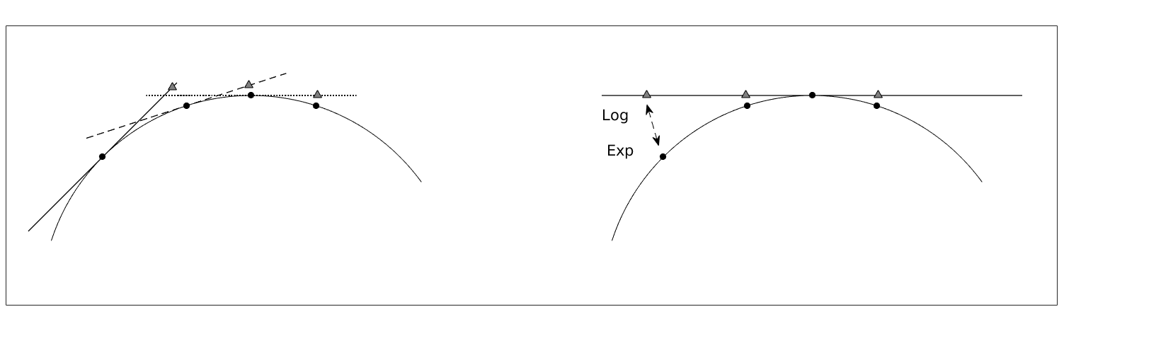
Algorithms 1 and 2 can be applied in practical applications, where the Riemannian exponential and logarithm mappings are known in explicit form. Applications in parametric model reduction that consider matrix manifolds include [31] (-data), [8, 73, 100] (Grassmann-data), [104] (Stiefel data) and [9, 81] (-data).
3.2 Interpolation via the Riemannian center of mass
As pointed out in Remark 2, interpolation of manifold data via the back and forth mapping of a complete data set of sample points between the manifold and its tangent space depends on the chosen base point. As a consequence, sample points may experience an uneven distortion under the projection onto the tangent space, see Fig. 3 (right). An approach that avoids this issue is to interpret interpolation as the task of finding suitably weighted Riemannian centers of mass. This concept was introduced in the context of geodesic finite elements in [90, 41].
The idea is as follows: The Riemannian center of mass1515 15 Here, we introduce this for discrete data sets; for centers w.r.t. a general mass distribution, see the original paper [55], Section 1. or Fréchet mean of a sample data set on a manifold with respect to the scalar weights , is defined as the minimizer(s) of the Riemannian objective function
where is the Riemannian distance of (5).
This definition generalizes the notion of the barycentric mean in Euclidean spaces.
However, on curved manifolds, the global center might not be unique. Moreover,
local minimizers may appear. For more details, see [55] and [4], which also give uniqueness criteria.
Interpolation is now performed by computing weighted Riemannian centers.
More precisely,
let be sampled parameter locations and let
, be the corresponding sample locations on .
Interpolation is within the convex hull of the samples.
Let be a suitable set of interpolation functions with , , say Lagrangians [90], splines [41] or radial basis functions [23]. Then, the interpolant at an unsampled parameter location is defined as the minimizer of
| (12) |
At a sample location , one has indeed that
which has the unique global minimum at .
Computing requires to solve a Riemannian optimization problem. The simplest approach is a gradient descent method [4, 3]. The gradient of the objective function in (12) is
| (13) |
see [55, Thm 1.2], [4, §2.1.5], [90, eq. (2.4)]. Hence, just like interpolation in the tangent space, the interpolation via the Riemannian center can be pursued only in applications, where the Riemannian logarithm can be computed. A generic gradient descent algorithm to compute the barycentric interpolant for a function reads as follows.
An implementation of this (type of) method for finding the Karcher mean in is discussed in [83]. Of course, Riemannian analogues to more sophisticated nonlinear optimization methods may also be employed, see [3].
In the context of model reduction, the benefits of interpolation via weighted Riemannian centers and the computational costs of solving the associated Riemannian optimization problem must be juxtaposed.
3.3 Additional approaches
A large variety of sophistications and further manifold interpolation techniques exists in the literature: The acceleration-minimizing property of cubic splines in the Euclidean space can be generalized to Riemannian manifolds in form of a variational problem [74, 30, 24, 93, 21, 87, 54], see also [80] and references therein. Moreover, the construction concepts of Bézier curves and the De Casteljau-algorithm [15] can be transferred to Riemannian manifolds [80, 59, 72, 1, 88]. Bézier curves in Euclidean spaces are polynomial splines that rely on a number of so-called control points. To obtain the value of a Bézier curve at time , a recursive sequence of straight-line convex combinations between pairs of control points must be computed. The transition of this technique to Riemannian manifolds is via replacing the inherent straight lines with geodesics [80]. Another option is to conduct the Bézier/De Casteljau-algorithm in the tangent space and to transfer the results to the manifold via a geodesic averaging of the spline arcs that were constructed in the tangent spaces at the first and the last control point, respectively, see [40].
Derivative information may also be incorporated in interpolation schemes on Riemannian manifolds. A Hermite-type method that is specifically tailored for interpolation problems on the Grassmann manifold is sketched in [7, §3.7.4]. General Hermitian manifold interpolation in compact, connected Lie groups with a bi-invariant metric has been considered in [52]. A practical approach to conduct first-order Hermite interpolation of data on arbitrary Riemannian manifolds is discussed in [103].
3.4 Quasi-linear extrapolation on matrix manifolds
In application scenarios, where both snapshot data of the full-order model and derivative information are at hand, various approaches have been suggested to exploit the latter. On the one hand, derivatives can be used for improving the ROMs accuracy and approximation quality by constructing POD bases that incorporate snapshots and snapshot derivatives [25, 48, 51, 99]. On the other hand, snapshot derivatives enable to parameterize the ROM bases and subspaces or to perform sensitivity analyses [97, 45, 44, 101]. In this section, we outline an approach to transfer the idea of extrapolation and parameterization via local linearizations to manifold-valued functions. The underlying idea is comparable to the trajectory piece-wise linear (TPWL) method [84]. Yet, TPWL linearizes the full-order model prior to the ROM projection, whereas here, we consider linearizing ROM building blocks like the reduced orthogonal bases, reduced subspaces or reduced system matrices.
A geometric first-order Taylor approximation
Any differentiable function can be linearized via a first-order Taylor expansion. A step ahead of size in direction gives When considering as a curve, then the first-order Taylor approximant is the straight line . Such first order linearization often serves for extrapolating a given nonlinear function in a neighborhood of a selected expansion point. For doing so, the starting point and the starting velocity must be available. This procedure translates to the manifold setting, when straight lines are replaced with geodesics.
Let be a scalar parameter and let be a curve on a submanifold . For given initial values and , the corresponding unique geodesic is expressed via the Riemannian exponential as
Example: Extrapolating POD basis matrices
As outlined in Section 1.1, snapshot POD works by collecting state vector snapshots, followed by an SVD of the snapshot matrix . Here, the matrix dimensions are , , . The objective is to approximate for a small based on the data , where is a point on the Stiefel manifold and is a tangent vector, see Section 4.4.1.
Differentiating the SVD. If the snapshot matrix function is smooth in the neighborhood of and if the singular values of are mutually distinct1616 16 This condition can be relaxed, see the results of [5, §7]., then the singular values and both the left and the right singular vectors are differentiable in for small enough. For brevity, let denote the derivative with respect to evaluated in and so forth. Let and let . Let and , denote the columns of and , respectively. It holds
| (14) | |||||
| (18) |
A proof can be found in [45]. Note that is skew-symmetric so that indeed . The above equations hold in approximative form for the truncated SVD. For convenience, assume that is now the truncated to columns.
Performing the Taylor extrapolation on . With at hand, can be approximated using the Stiefel exponential: , see Algorithm 7.The process is illustrated in Fig. 4.

Note that when the -dependency is real-analytic, then the Euclidean Taylor expansion
| (19) |
converges to an orthogonal matrix . Yet, when truncating the Taylor series, we leave the Stiefel manifold. In particular, the columns of the first order approximation are not orthonormal, i.e. for . By construction, the Stiefel geodesic features the same starting velocity and thus matches the Taylor series up to terms of second order. In addition, it respects the geometric structure of the Stiefel manifold and thus preserves column-orthonormality for every .
4 Matrix manifolds of practical importance
In this section, we discuss the matrix manifolds that feature most often in practical applications in the context of model reduction. For each manifold under consideration, we recap, if applicable
- •
the representation of points/locations in numerical schemes.
- •
the representation of tangent vectors in numerical schemes.
- •
the most common Riemannian metrics.
- •
how to compute distances, geodesics and the Riemannian exponential and logarithm mappings.
4.1 The general linear group
This section is devoted to the general linear group of invertible square matrices. In model reduction, regular matrices appear for example as (reduced) system matrices in LTI and discretized PDE systems [9, 31, 76] and parameterizations have to be such that matrix regularity is preserved. In addition, the discussion of the seemingly simple matrix manifold is important, because it is the fundamental matrix Lie Group from which all other matrix Lie groups are derived. Moreover, it provides the background for understanding quotient spaces of , see Subsection 2.5 and also [20, 96]. A short summary on the Riemannian geometry of is given in [82, §6].
4.1.1 Introduction and data representation in numerical schemes
Because , is an open subset of the -dimensional vector space and is thus an -dimensional differentiable manifold, see [63, Examples 1.22–1.27]. The matrix manifold is disconnected as it decomposes into two connected components, namely the regular matrices of positive determinant and the regular matrices of negative determinant.
Because is an open subset of the vector space , the tangent space at a location is simply . For , the Lie algebra is , so that the Lie group exponential is the standard matrix exponential . From the Lie group perspective (10), the tangent space at an arbitrary point is to be considered as the set , even though this set coincides with .
4.1.2 Distances and geodesics
The obvious choice for a Riemannian metric on is to use the inner product from the ambient Euclidean matrix space, i.e.,
for and .
In many applications, it is more appropriate to consider metrics with certain invariance properties.1717 17 “Eulerian motion of a rigid body can be described as motion along geodesics in the group of rotations of three-dimensional euclidean space provided with a left-invariant Riemannian metric. A significant part of Euler’s theory depends only upon this invariance, and therefore can be extended to other groups.”[11, Appendix 2, p. 318] A left-invariant metric can be obtained from the standard metric via
| (20) |
When formally considering as left-translates of tangent vectors , then this metric satisfies . Alternatively, , which explains the name ‘left-invariant’.
The Riemannian exponential and logarithm for the flat metric
When equipped with the Euclidean metric, is flat: since the tangent space is the full matrix space , the geodesic equation (7) requires the acceleration of a geodesic curve to vanish completely. Hence, the geodesic that starts from with velocity is the straight line . Note that the curve may leave the manifold for some as it may hit a matrix with zero determinant. The formulae for the Riemannian exponential and logarithm mapping at a base point are
| (21) | |||||
| (22) |
In (21), denotes a suitably small open neighborhood around such that for all .
The Riemannian exponential for the left-invariant metric on GL(n)
The left-invariant metric induces a non-flat geometry on . Formulae for the covariant derivatives and the corresponding geodesics are derived in [10, Thm. 2.14]. The counterparts w.r.t. the right-invariant metrics can be found in [96]. Given a base point and a starting velocity , the associated geodesic is
| (23) |
The Riemannian exponential is
| (24) | |||||
The author is not aware of a closed formula for the inverse map, i.e., the Riemannian logarithm for the left-invariant metric, see also the discussion in [96, §4.5]. The thesis [82, §6.2] introduces a Riemannian shooting method for computing the Riemannian logarithm w.r.t. the left-invariant metric.
An important special case
For tangent vectors with normal , i.e., , it holds that the matrices and commute. Therefore, according to (38), and the Riemannian exponential reduces to
The Riemannian logarithm is
where is a domain such that a suitable branch of the matrix logarithm is well-defined. These expressions are sometimes encountered in the literature as the Riemannian exponential and logarithm mappings. Yet, one should be aware of the fact that they hold under special circumstances.
4.2 The orthogonal group
This section is devoted to the orthogonal group of orthogonal -by- matrices. In parametric model reduction, such matrices may appear as eigenvector matrices in symmetric EVD problems.
4.2.1 Introduction and data representation in numerical schemes
The orthogonal group is . The manifold structure of can be established via Theorem 2, see also Example 1. The orthogonal group decomposes into two connected components, namely the orthogonal matrices with determinant and the orthogonal matrices with determinant . The former constitute the special orthogonal group . The orthogonal group is a closed subgroup of the Lie group and thus itself a Lie group (Section 2.5). The tangent space at the identity forms the Lie algebra associated with the Lie group . It coincides with the Lie algebra of and as such is denoted by , [43, §3.3, 3.4]. The Lie algebra of is precisely the vector space of skew-symmetric matrices, . According to (10), the tangent space at an arbitrary location is given by the translates (by left-multiplication) of the Lie algebra
which is the same as . The Lie exponential is
| (25) |
This restriction is a surjective map, see Appendix A. The dimensions of both and are .
4.2.2 Distances and geodesics
We follow up on the discussion in Section 4.1.1. For the orthogonal group, the Euclidean metric and the left-invariant metric coincide: Let . Then,
In fact, the metric is also right-invariant, which makes it a bi-invariant metric, see [6, §2]. Bi-invariant metrics are important, because for Lie groups endowed with bi-invariant metrics, the Lie exponential map and the Riemannian exponential map at the identity coincide [6, Thm. 2.27, p. 40].
The Riemannian exponential and logarithm maps on O(n)
The Riemannian -exponential at a base point sends a tangent vector to the endpoint of a geodesic that starts from with velocity vector . Therefore, it provides at the same time an expression for the geodesic curves on . A formula for computing the Riemannian -exponential was derived in [33, §2.2.2]. Given , it holds
| (26) |
This result is also immediate from abstract Lie theory, see [6, Eq. (2.2) & Thm. 2.27].1818 18 The Lie exponential is , which is in the case at hand the Riemannian exponential at the identity, . This translates to any other location via [6, Eq. (2.2)] as follows: Pick any and consider the mapping “left-multiplication by Q”, i.e., . Then, the differential is . Because is an isometry, which gives and thus (26). The corresponding Riemmanian logarithm on is
| (27) |
and is well defined on a neighborhood around such that for all , the orthogonal matrix does not feature as an eigenvalue.
The Riemannian distance between orthogonal matrices
For given from the same connected component of , consider the EVD . Because is orthogonal, it holds and we assume that . The Riemannian distance is
The compact Lie group is a geodesically complete Riemannian manifold [6, Hopf-Rinow-Theorem, p. 31], and each two points of can be joined by a minimal geodesic.
4.3 The matrix manifold of symmetric positive definite matrices
This section is devoted to the matrix manifold of real, symmetric positive-definite -by- matrices. In model reduction, such matrices appear for example as (reduced) system matrices in second-order parametric ODEs. For example, in linear structural or electrical dynamical systems, mass, stiffness and damping matrices are usually in , [9, §4.2]. Moreover, positive definite matrices arise as Gramians of reachable and observable LTI systems in the context of balanced truncation [17]. Related is the manifold of positive semi-definite matrices of fixed rank. It is investigated in [20, 96, 64]. An application in the context of model reduction features in [65].
4.3.1 Introduction and data representation in numerical schemes
The set
is an open subset of the metric Hilbert space of symmetric matrices. As such, it is a differentiable manifold [19, §6]. Moreover, it forms a convex cone [34, Example 2, p. 8], [68, §2.3], and can be realized as a quotient . The latter is based on the fact that for , matrix factorizations with are invariant under orthogonal transformations , , [20, §2, p.3].
Since is an open subset of the vector space , the tangent space is simply
| (28) |
The dimensions of both and are .
There is a smooth one-to-one correspondence between and . That is, every positive definite matrix can be written as the matrix exponential of a unique symmetric matrix, [36, Lem. 18.7, p. 472]. Put in different words, when restricted to , the standard matrix exponential
is a diffeomorphism, its inverse is the standard principal matrix logarithm
see also [12, Thm. 2.8]. The group acts on via congruence transformations
| (29) |
For additional background on , see [69, 70, 78]. Applications in computer vision are presented in [28, 56].
4.3.2 Distances and geodesics
The literature knows a large variety of distance measures on , see [53, Table 3.1, p. 56]. Yet, there are essentially two choices that are associated with inner products on the tangent space of and thus induce Riemannian geometries on the manifold : the so-called natural metric and the log-Euclidean metric. Let and let be two tangent vectors.
- •
The natural metric is
see [19, §6, p. 201], [20]. It also goes by the name trace matric, [61, §XII.1, p.322]. In statistical applications, it is usually called the affine-invariant metric [67, 79].1919 19 The motivation is as follows: if , is an affine transformation of a random vector , then the mean is transformed to and the covariance matrix undergoes a congruence transformation .
- •
For the natural metric, it is more appropriate to consider as the tangent space at the identity and the tangent space at an arbitrary location as , which, of course, is nothing but a reparameterization of . From this perspective, we have for tangent vectors that
The congruence transformations (29) are isometries of with respect to the natural metric, [61, Thm. XII.1.1, p. 324], [19, Lem. 6.1.1, p. 201]. See also the discussion in [79, §3].
By a standard pullback construction from differential geometry [32, Def. 2.2, Example 2.5], the log-Euclidean metric transfers the inner product on to via the matrix logarithm . In [12, eq. (3.5)], the authors take this construction one step further and use the --correspondence to define a multiplication that turns into a Lie group and, eventually, into a vector space. As such, it is a flat manifold, i.e. a Riemannian manifold with zero curvature. In this way, the computational challenges that come with dealing with data on nonlinear manifolds are circumvented.
Which metric is to be preferred is problem-dependent, see the various contributions in [92] and [66]. Since the natural metric arises canonical both from the geometric approach, [61, §XII.1], and the matrix-algebraic approach [19, §6] and since staying with the standard matrix multiplication is consistent with the setting of solving dynamical systems in model reduction applications, we restrict the discussion of the Riemannian exponential and logarithm to the geometry that is based on the natural metric.
The SPD(n) exponential
The Riemannian -exponential at a base point sends a tangent vector to the endpoint of a geodesic that starts from with velocity vector . Therefore, it provides at the same time an expression for the geodesic curves on with respect to the natural metric. Formulae for computing the -exponential can be found in [20], [79]. Readers preferring a matrix-analytic approach are referred to [19, §6].
Here, denotes the matrix square root of , see Appendix A.
The SPD(n) logarithm
The Riemannian -logarithm at a base point finds for another point an -tangent vector such that the geodesic that starts from with velocity reaches after an arc length of . Therefore, it provides for two given data points
- •
a solution to the geodesic endpoint problem: a geodesic that starts from and ends at .
- •
the Riemannian distance between the given points .
Formulae for computing the -logarithm can be found in [20], [79].
Both Algorithms 5 and 6 require to compute the spectral decomposition of -by--matrices. The computational effort is . In the context of parametric model reduction, the Riemannian exponential and logarithm maps are usually required for reduced matrix operators [9]. If denotes the dimension of the full state vectors and denotes the dimension of the reduced state vectors, then matrix exponentials for -by--matrices are required, so that the computational effort reduces to .
4.4 The Stiefel manifold
This section is devoted to the Stiefel manifold of rectangular column-orthogonal -by- matrices, . Points may be considered as orthonormal bases of cardinality , or -frames in . In model reduction, such matrices appear as orthogonal coordinate systems for low-order ansatz spaces that usually stem from a proper orthogonal decomposition or a singular value decomposition of given input solution data. Modeling data on the Stiefel manifold corresponds to data processing for orthonormal bases and thus allows for example for interpolation/parameterization of POD subspace bases. The most important use case in model reduction is where the Stiefel matrices are tall and skinny, i.e., . Interpolation problems on the Stiefel manifold have not yet been considered in the model reduction context. The reference [59] discusses interpolation of Stiefel data, however with using quasi-geodesics rather than geodesics. The work [103] includes numerical experiments for interpolating orthogonal frames on the Stiefel manifold that relies the canonical Riemannian Stiefel logarithm [82, 102].
4.4.1 Introduction and data representation in numerical schemes
The Stiefel manifold is the compact, homogeneous matrix manifold of column-orthogonal matrices
The manifold structure can be directly established via Theorem 2 in a similar way as in Example 1. An alternative approach is via Example 3, where is identified with the quotient space under actions of the closed subgroup . Two square orthogonal matrices in are identified as the same point on , if their first columns coincide, see [33, §2.4].
4.4.2 Distances and geodesics
Let be a point and let , be tangent vectors. There are two standard metrics on the Stiefel manifold.
- •
The Euclidean metric on is the one inherited from the ambient :
- •
The canonical metric on
is derived from the quotient representation of the Stiefel manifold.
The canonical metric counts the independent coordinates2020 20 i.e., the upper triangular entries of the skew-symmetric and the entries of of of a tangent vector equally, when measuring the length of a tangent vector , while the Euclidean metric disregards the skew-symmetry of [33, §2.4]. Recall that different metrics entail different measures for the lengths of curves and thus different formulae for geodesics.
The Stiefel exponential
The Riemannian Stiefel exponential at a base point sends a Stiefel tangent vector to the endpoint of a geodesic that starts from with velocity vector . Therefore, it provides at the same time an expression for geodesic curves on .
A closed-form expression for the Stiefel exponential w.r.t. Euclidean metric is included in [33, §2.2.2],
In [50], an alternative formula is derived that features only matrix exponentials of skew-symmetric matrices. An efficient algorithm for computing the Stiefel exponential w.r.t. the canonical metric was derived in [33, §2.4.2]:
In applications, where needs to be evaluated for various parameters as in in the example of Section 3.4, steps 1.–3. should be computed a priori (offline). Apart from elementary matrix multiplications, the algorithm requires to compute the standard matrix exponential of a skew-symmetric matrix. This however, is for a -by--matrix and does not scale in the dimension . With the usual assumption of model reduction that , the computational effort is .
The Stiefel logarithm
The Riemannian Stiefel logarithm at a base point finds for another point a Stiefel tangent vector such that the geodesic that starts from with velocity reaches after an arc length of . Therefore, it provides for two given data points
- •
a solution to the geodesic endpoint problem: a geodesic that starts from and ends at .
- •
the Riemannian distance between the given points .
An efficient algorithm for computing the Stiefel logarithm w.r.t. the canonical metric was derived in [102].
The analysis in [102] shows that the algorithm is guaranteed to converge if the input data points are at most a Euclidean distance of apart. In this case, the algorithm exhibits a linear rate of convergence that depends on but is smaller than . In practice, the algorithm seems to converge, whenever the initial is such that its standard matrix logarithm is well-defined. Note that two points on can at most be a Euclidean distance of away from each other.
Apart from elementary matrix multiplications, the algorithm requires to compute the standard matrix logarithm of an orthogonal -by--matrix and the standard matrix exponential of a skew-symmetric -by--matrix at every iteration . Yet, these operations are independent of the dimension . With the usual assumption of model reduction that , the computational effort is .
For the Stiefel manifold equipped with the Euclidean metric, methods for calculating the Stiefel logarithm are introduced in [22].
4.5 The Grassmann manifold
This section is devoted to the Grassmann manifold of -dimensional subspaces of for . Every point , i.e., every subspace may be represented by selecting a basis with . In numerical schemes, we work exclusively with orthonormal bases. In this way, points on the Grassmann manifold are to be represented by points on the Stiefel manifold via . For details and theoretical background, see the references [2, 3, 33]. Subspaces and Grassmann manifolds play an important role in projection-based parametric model reduction, [8, 73, 100, 86] and in Krylov subspace approaches [17]. Modeling data on the Grassmann manifold corresponds to data processing for subspaces and thus allows for example for the interpolation/parameterization of POD subspaces. The most important use case in model reduction is where the subspaces are of low dimension when compared to the surrounding state space, i.e., .
4.5.1 Introduction and data representation in numerical schemes
The set of all -dimensional subspaces forms the Grassmann manifold
The Grassmann manifold is a quotient of under the action of the Lie subgroup . Two matrices are in the same -orbit, if and only if the first columns of and span the same subspace and the tailing columns span the corresponding orthogonal complement subspace. Theorem 11 applies and shows that is a homogeneous manifold.
Alternatively, the Grassmann manifold can be realized as a quotient manifold of the Stiefel manifold with the help of Theorem 9,
| (32) |
where the -orbits are . A matrix is called a matrix representative of a subspace , if . The orbit and the subspace are to be considered as the same object. For any matrix representative of the tangent space of at is represented by
Every tangent vector may be written as
| (33) | |||||
| (34) |
where in the latter case, is such that is a square orthogonal matrix. The dimension of both and is .
4.5.2 Distances and geodesics
A metric on can be obtained via making use of the fact that the Grassmannian is a quotient of the Stiefel manifold. Alternatively, one can restrict the standard inner matrix product to the Grassmann tangent space. In the case of the Grassmannian, both approaches lead to the same metric
see [33, §2.5].
The Grassmann exponential
The Riemannian Grassmann exponential at a base point sends a Grassmann tangent vector to the endpoint of a geodesic that starts from with velocity vector . Therefore, it provides at the same time an expression for the geodesic curves on . An efficient algorithm for computing the Grassmann exponential was derived in [33, §2.5.1]:
Apart from elementary matrix multiplications, the algorithm requires to compute the singular value decomposition of an -by--matrix. The computational effort is .
The Grassmann logarithm
The Riemannian Grassmann logarithm at a base point finds for another point a Grassmann tangent vector such that the geodesic that starts from with velocity reaches after an arc length of . Therefore, it provides for two given data points
- •
a solution to the geodesic endpoint problem: a geodesic that starts from and ends at .
- •
the Riemannian distance between the given points .
An algorithm for computing the Grassmann logarithm is stated implicitly in [2, §3.8, p. 210]. The reference [37] features expressions for the Grassmann exponential and the corresponding logarithm that formally work with Grassmann representatives in but also keep the computational effort . The reference [81, §4.3] gives the corresponding mappings after identifying subspaces with orthoprojectors, see also [16].
The composition is the identity on , wherever it is defined. Yet, on the level of the actual matrix representatives, the operation
produces a matrix . Directly recovering the input matrix can be achieved via a Procrustes-type preprocessing step, where is replaced with , . This leads to:
An additional advantage of the modified Grassmann logarithm is that the matrix inversion is avoided. In fact, it is replaced by the SVD that is used to solve the Procrustes problem . The SVD exists also if does not have full rank.
Distances between subspaces
The Riemannian logarithm provides the distance between two subspaces as follows: First, compute , then compute . In practice, however, this boils down to computing the singular values of the matrix , which can be seen as follows. By Algorithm 11, , where the ’s are the singular values of . These match precisely the square roots of the eigenvalues of . Using the SVD of the square matrix as in steps 1&2 of Algorithm 11, the eigenvalues of can be read off from
so that , when consistently ordered. As a consequence, , which implies
| (35) |
where and are the singular values of and , respectively.
The numerical linear algebra literature knows a variety of distance measures for subspaces. Essentially, all of them are based on the principal angles [33, §2.5.1, §4.3]. The principal angles (or canonical angles) between two subspaces are defined recursively by
The principal angles can be computed via , where is the th singular value of [39, §6.4.3]. Hence, the Riemannian subspace distance (35) expressed in terms of the principal angles is precisely
| (36) |
In particular, (36) shows that any two points on can be connected by a geodesic of length at most , see also [98, Thm 8(b)].
Appendix A Appendix
The matrix exponential and logarithm
The standard matrix exponential and matrix logarithm are defined via the power series
| (37) |
For , is invertible with inverse . The following restrictions of the exponential map are important:
The former is a diffeomorphism [78, Thm. 2.8], the latter is a differentiable, surjective map [38, §. 3.11, Thm. 9]. For additional properties and efficient methods for numerical computation, see [47, §10, 11].
A few properties of the exponential function for real or complex numbers carry over to the matrix exponential. However, since matrices do not commute, the standard exponential law is replaced by
| (38) | |||||
where is the commutator bracket, or Lie bracket. This is Dynkin’s formula for the Baker-Campbell-Hausdorff series, see [85, §1.3, p. 22]. From a theoretical point of view, it is important that all terms in this series can be expressed in terms of the Lie bracket. A special case is
Matrix square roots and the polar decomposition
Every has a unique matrix square root in , i.e., a matrix denoted by with the property . This square root can be obtained via an EVD by setting
where , and are the eigenvalues of . Every can be uniquely decomposed into an orthogonal matrix times a symmetric positive definite matrix,
The polar factors can be constructed via taking the square root of the assuredly positive definite matrix and subsequently setting and . Because the restriction of to the symmetric matrices is a diffeomorphism onto , there is a unique with . For details, see [43, Thm. 2.18].
The Procrustes problem
Let . The Procrustes problem aims at finding an orthogonal transformation such that is the minimizer of
The optimal is , where , see [39].
References
- [1] P.-A. Absil, P.-Y. Gousenbourger, P. Striewski, and B. Wirth, Differentiable piecewise-Bézier surfaces on Riemannian manifolds, SIAM Journal on Imaging Sciences, 9 (2016), pp. 1788–1828.
- [2] P.-A. Absil, R. Mahony, and R. Sepulchre, Riemannian geometry of Grassmann manifolds with a view on algorithmic computation, Acta Applicandae Mathematica, 80 (2004), pp. 199–220.
- [3] , Optimization Algorithms on Matrix Manifolds, Princeton University Press, Princeton, New Jersey, 2008.
- [4] B. Afsari, R. Tron, and R. Vidal, On the convergence of gradient descent for finding the Riemannian center of mass, SIAM Journal on Control and Optimization, 51 (2013), pp. 2230–2260.
- [5] D. Alekseevsky, A. Kriegl, P. W. Michor, and M. Losik, Choosing roots of polynomials smoothly, Israel Journal of Mathematics, 105 (1998), pp. 203–233.
- [6] M. M. Alexandrino and R. G. Bettiol, Lie Groups and Geometric Aspects of Isometric Actions, Springer International Publishing, Cham, 2015.
- [7] D. Amsallem, Interpolation on Manifolds of CFD-based Fluid and Finite Element-based Structural Reduced-order Models for On-line Aeroelastic Prediction, PhD thesis, Stanford University, 2010.
- [8] D. Amsallem and C. Farhat, Interpolation method for adapting reduced-order models and application to aeroelasticity, AIAA Journal, 46 (2008), pp. 1803–1813.
- [9] , An online method for interpolating linear parametric reduced-order models, SIAM Journal on Scientific Computing, 33 (2011), pp. 2169–2198.
- [10] E. Andruchow, G. Larotonda, L. Recht, and A. Varela, The left invariant metric in the general linear group, Journal of Geometry and Physics, 86 (2014), pp. 241 – 257.
- [11] V. Arnol’d, Mathematical Methods of Classical Mechanics, Graduate Texts in Mathematics, Springer, New York, 1997.
- [12] V. Arsigny, P. Fillard, X. Pennec, and N. Ayache, Geometric means in a novel vector space structure on symmetric positive-definite matrices., SIAM Journal on Matrix Analysis Applications, 29 (2006), pp. 328–347.
- [13] P. Astrid, S. Weiland, K. Willcox, and T. Backx, Missing points estimation in models described by proper orthogonal decomposition, IEEE Transactions on Automatic Control, 53 (2008), pp. 2237–2251.
- [14] M. Barrault, Y. Maday, N. Nguyen, and A. Patera, An “empirical interpolation” method: Application to efficient reduced-basis discretization of partial differential equations, Comptes Rendus Mathématique. Académie des Sciences. Paris, I 339 (2004), pp. 667–672.
- [15] R. H. Bartels, J. C. Beatty, and B. A. Barsky, An Introduction to Splines for Use in Computer Graphics and Geometric Modeling, Morgan Kaufmann Series in Comp, Elsevier Science, 1995.
- [16] E. Batzies, K. Hüper, L. Machado, and F. Silva Leite, Geometric mean and geodesic regression on Grassmannians, Linear Algebra and Its Applications, 466 (2015), pp. 83–101.
- [17] P. Benner, S. Gugercin, and K. Willcox, A survey of projection-based model reduction methods for parametric dynamical systems, SIAM Review, 57 (2015), pp. 483–531.
- [18] A. V. Bernstein and A. P. Kuleshov, Tangent bundle manifold learning via Grassmann & Stiefel eigenmaps, arXiv preprint arXiv:1212.6031, (2012).
- [19] R. Bhatia, Positive Definite Matrices, Princeton Series in Applied Mathematics, Princeton University Press, Princeton, New Jersey, 2007.
- [20] S. Bonnabel and R. Sepulchre, Riemannian metric and geometric mean for positive semidefinite matrices of fixed rank, SIAM Journal on Matrix Analysis and Applications, 31 (2009), pp. 1055–1070.
- [21] N. Boumal and P.-A. Absil, A discrete regression method on manifolds and its application to data on SO(n), IFAC Proceedings Volumes, 44 (2011), pp. 2284 – 2289. 18th IFAC World Congress.
- [22] D. Bryner, Endpoint geodesics on the Stiefel manifold embedded in Euclidean space, SIAM Journal on Matrix Analysis and Applications, 38 (2017), pp. 1139–1159.
- [23] M. D. Buhmann, Radial Basis Functions, vol. 12 of Cambridge Monographs on Applied and Computational Mathematics, Cambridge University Press, Cambridge, UK, 2003.
- [24] M. Camarinha, F. S. Leite, and P. Crouch, On the geometry of riemannian cubic polynomials, Differential Geometry and its Applications, 15 (2001), pp. 107 – 135.
- [25] K. Carlberg and C. Farhat, A low-cost, goal-oriented ‘compact proper orthogonal decomposition’ basis for model reduction of state systems, International Journal for Numerical Methods in Engineering, 86 (2011), pp. 381–402.
- [26] R. Chakraborty and B. C. Vemuri, Statistics on the (compact) Stiefel manifold: Theory and applications. arXiv:1708.00045v1, 2017.
- [27] S. Chaturantabut and D. Sorensen, Nonlinear model reduction via discrete empirical interpolation, SIAM Journal on Scientific Computing, 32 (2010), pp. 2737–2764.
- [28] A. Cherian and S. Sra, Positive definite matrices: Data representation and applications in computer vision, in Algorithmic Advances in Riemannian Geometry and Applications: For Machine Learning, Computer Vision, Statistics, and Optimization, H. Q. Minh and V. Murino, eds., Springer International Publishing, Cham, 2016, pp. 93–114.
- [29] Y. Choi, D. Amsallem, and C. Farhat, Gradient-based constrained optimization using a database of linear reduced-order models, arXiv, arXiv:1506.07849v1 (2015), pp. 1–28.
- [30] P. Crouch and F. S. Leite, The dynamic interpolation problem: On Riemannian manifolds, Lie groups, and symmetric spaces, Journal of Dynamical and Control Systems, 1 (1995), pp. 177–202.
- [31] J. Degroote, J. Vierendeels, and K. Willcox, Interpolation among reduced-order matrices to obtain parameterized models for design, optimization and probabilistic analysis, International Journal for Numerical Methods in Fluids, 63 (2010), pp. 207–230.
- [32] M. P. do Carmo, Riemannian Geometry, Mathematics: Theory & Applications, Birkhäuser Boston, 1992.
- [33] A. Edelman, T. A. Arias, and S. T. Smith, The geometry of algorithms with orthogonality constraints, SIAM Journal on Matrix Analysis and Applications, 20 (1998), pp. 303–353.
- [34] J. Faraut and A. Koranyi, Analysis on Symmetric Cones, Oxford Mathematical Monographs, Oxford University Press, New York, 1994.
- [35] T. Franz, R. Zimmermann, S. Görtz, and N. Karcher, Interpolation-based reduced-order modeling for steady transonic flows via manifold learning, International Journal of Computational Fluid Mechanics, Special Issue on Reduced Order Modeling, 228 (2014), pp. 106–121.
- [36] J. H. Gallier, Geometric methods and applications: for computer science and engineering, Texts in Applied Mathematics, Springer, New York, 2011.
- [37] K. A. Gallivan, A. Srivastava, X. Liu, and P. Van Dooren, Efficient algorithms for inferences on Grassmann manifolds, in IEEE Workshop on Statistical Signal Processing, 2003, pp. 315–318.
- [38] R. Godement and U. Ray, Introduction to the Theory of Lie Groups, Universitext, Springer International Publishing, 2017.
- [39] G. H. Golub and C. F. Van Loan, Matrix Computations, The John Hopkins University Press, Baltimore, 4th ed., 2013.
- [40] P.-Y. Gousenbourger, E. Massart, and P.-A. Absil, Data fitting on manifolds with composite Bézier-like curves and blended cubic splines, Journal of Mathematical Imaging and Vision, online (2018), pp. 1–27.
- [41] P. Grohs, Quasi-interpolation in Riemannian manifolds, IMA Journal of Numerical Analysis, 33 (2013), pp. 849–874.
- [42] B. Haasdonk and M. Ohlberger, Efficient reduced models and a-posteriori error estimation for parametrized dynamical systems by offline/online decomposition, Mathematical and Computer Modelling of Dynamical Systems, 17 (2011), pp. 145–161.
- [43] B. C. Hall, Lie Groups, Lie Algebras, and representations: An elementary introduction, Springer Graduate texts in Mathematics, Springer–Verlag, New York – Berlin – Heidelberg, 2nd ed., 2015.
- [44] A. Hay, J. Borggaard, I. Akhtar, and D. Pelletier, Reduced-order models for parameter dependent geometries based on shape sensitivity analysis, Journal of Computational Physics, 229 (2010), pp. 1327–1352.
- [45] A. Hay, J. T. Borggaard, and D. Pelletier, Local improvements to reduced-order models using sensitivity analysis of the proper orthogonal decomposition, Journal of Fluid Mechanics, 629 (2009), pp. 41–72.
- [46] U. Helmke and J. B. Moore, Optimization and Dynamical Systems, Communications & Control Engineering, Springer–Verlag, London, 1994.
- [47] N. J. Higham, Functions of Matrices: Theory and Computation, Society for Industrial and Applied Mathematics, Philadelphia, PA, USA, 2008.
- [48] M. Hinze and S. Volkwein, Proper orthogonal decomposition surrogate models for nonlinear dynamical systems: Error estimates and suboptimal control, in Dimension Reduction of Large-Scale Systems, vol. 45 of Lecture Notes in Computational Science and Engineering, Springer, Berlin–Heidelberg, 2005, pp. 261–306.
- [49] K. Hüper, M. Kleinsteuber, and F. Silva Leite, Rolling Stiefel manifolds, International Journal of Systems Science, 39 (2008), pp. 881–887.
- [50] K. Hüper and F. Ullrich, Real Stiefel manifolds: An extrinsic point of view, in 2018 13th APCA International Conference on Automatic Control and Soft Computing (CONTROLO), June 2018, pp. 13–18.
- [51] K. Ito and S. S. Ravindran, A reduced-order method for simulation and control of fluid flows, Journal of Computational Physics, 143 (1998), pp. 403–425.
- [52] J. Jakubiak, F. S. Leite, and R. Rodrigues, A two-step algorithm of smooth spline generation on riemannian manifolds, Journal of Computational and Applied Mathematics, 194 (2006), pp. 177–191.
- [53] S. Jayasumana, R. Hartley, and M. Salzmann, Kernels on Riemannian manifolds, in Riemannian computing in computer vision, A. Srivastava and P. K. Turaga, eds., Springer International Publishing, 2015, pp. 45–67.
- [54] H. K. R. Kim, I. L. Dryden, Smoothing splines on riemannian manifolds, with applications to 3D shape space. arXiv:1801.04978v2, 2018.
- [55] H. Karcher, Riemannian center of mass and mollifier smoothing, Communications on Pure and Applied Mathematics, 30 (1977), pp. 509–541.
- [56] H. J. Kim, N. Adluru, B. B. Bendlin, S. C. Johnson, B. C. Vemuri, and V. Singh, Canonical correlation analysis on SPD(n) manifolds, in Riemannian computing in computer vision, A. Srivastava and P. K. Turaga, eds., Springer International Publishing, 2015, pp. 69–100.
- [57] S. Kobayashi and K. Nomizu, Foundations of Differential Geometry, vol. I of Interscience Tracts in Pure and Applied Mathematics no. 15, John Wiley & Sons, New York – London – Sidney, 1963.
- [58] , Foundations of Differential Geometry, vol. II of Interscience Tracts in Pure and Applied Mathematics no. 15, John Wiley & Sons, New York – London – Sidney, 1969.
- [59] K. A. Krakowski, L. Machado, F. Silva Leite, and J. Batista, Solving interpolation problems on Stiefel manifolds using quasi-geodesics, in Pré-Publicaçiões do Departamento de Matemática, no. 15–36, Universidade de Coimbra, 2015.
- [60] W. Kühnel, Differential Geometry: Curves - Surfaces - Manifolds, Student mathematical library, American Mathematical Society, 2006.
- [61] S. Lang, Fundamentals of Differential Geometry, Graduate Texts in Mathematics, Springer New York, 2001.
- [62] J. M. Lee, Riemannian Manifolds: an Introduction to Curvature, Springer Verlag, New York – Berlin – Heidelberg, 1997.
- [63] , Introduction to Smooth Manifolds, Graduate Texts in Mathematics, Springer New York, 2012.
- [64] E. Massart and P.-A. Absil, Quotient geometry with simple geodesics for the manifold of fixed-rank positive-semidefinite matrices, Tech. Rep. UCL-INMA-2018.06, University of Louvain, 2018.
- [65] E. Massart, P.-Y. Gousenbourger, T. S. Nguyen, T. Stykel, and P.-A. Absil, Interpolation on the manifold of fixed-rank positive-semidefinite matrices for parametric model order reduction: preliminary results, Tech. Rep. UCL-INMA-2018.13, University of Louvain, 2018.
- [66] H. Q. Minh and V. Murino, Algorithmic Advances in Riemannian Geometry and Applications: For Machine Learning, Computer Vision, Statistics, and Optimization, Advances in Computer Vision and Pattern Recognition, Springer International Publishing, Cham, 2016.
- [67] , From covariance matrices to covariance operators: Data representation from finite to infinite-dimensional settings, in Algorithmic Advances in Riemannian Geometry and Applications: For Machine Learning, Computer Vision, Statistics, and Optimization, H. Q. Minh and V. Murino, eds., Springer International Publishing, Cham, 2016, pp. 115–143.
- [68] M. Moakher, A differential geometric approach to the geometric mean of symmetric positive-definite matrices, SIAM Journal on Matrix Analysis and Applications, 26 (2005), pp. 735–747.
- [69] M. Moakher and P. G. Batchelor, Symmetric positive-definite matrices: From geometry to applications and visualization, in Visualization and Processing of Tensor Fields, J. Weickert and H. Hagen, eds., Mathematics and Visualization, Springer, Berlin – Heidelberg, 2006, pp. 285–298.
- [70] M. Moakher and M. Zéraï, The Riemannian geometry of the space of positive-definite matrices and its applications to the regularization of positive-definite matrix-valued data., Journal of Mathematical Imaging and Vision, 40 (2011), pp. 171–187.
- [71] M. Morzyński, W. Stankiewicz, B. R. Noack, R. King, F. Thiele, and G. Tadmor, Continuous mode interpolation for control-oriented models of fluid flow, in Active Flow Control, R. King, ed., Springer, Berlin – Heidelberg, 2007, pp. 260–278.
- [72] E. Nava-Yazdani and K. Polthier, De Casteljau’s algorithm on manifolds, Computer Aided Geometric Design, 30 (2013), pp. 722–732.
- [73] T. S. Nguyen, A real time procedure for affinely dependent parametric model order reduction using interpolation on Grassmann manifolds, International Journal for Numerical Methods in Engineering, 93 (2013), pp. 818–833.
- [74] L. Noakes, G. Heinzinger, and B. Paden, Cubic splines on curved spaces, IMA Journal of Mathematical Control and Information, 6 (1989), pp. 465–473.
- [75] M. Ohlberger and F. Schindler, Error control for the localized reduced basis multi-scale method with adaptive on-line enrichment, SIAM Journal on Scientific Computing, 37 (2015), pp. A2865–A2895.
- [76] H. Panzer, J. Mohring, R. Eid, and B. Lohmann, Parametric model order reduction by matrix interpolation, Automatisierungstechnik, 58 (2010), pp. 475–484.
- [77] B. Peherstorfer, D. Butnaru, K. Willcox, and H.-J. Bungartz, Localized discrete empirical interpolation method, SIAM Journal on Scientific Computing, 36 (2014), pp. A168–A192.
- [78] X. Pennec, Intrinsic statistics on Riemannian manifolds: Basic tools for geometric measurements, Journal of Mathematical Imaging and Vision, 25 (2006), p. 127.
- [79] X. Pennec, P. Fillard, and N. Ayache, A Riemannian framework for tensor computing, International Journal of Computer Vision, 66 (2006), pp. 41–66.
- [80] T. Popiel and L. Noakes, Bézier curves and C2 interpolation in Riemannian manifolds, Journal of Approximation Theory, 148 (2007), pp. 111–127.
- [81] I. U. Rahman, I. Drori, V. C. Stodden, D. L. Donoho, and P. Schröder, Multiscale representations for manifold-valued data, SIAM Journal on Multiscale Modeling and Simulation, 4 (2005), pp. 1201–1232.
- [82] Q. Rentmeesters, Algorithms for data fitting on some common homogeneous spaces, PhD thesis, Université Catholique de Louvain, Louvain, Belgium, 2013.
- [83] Q. Rentmeesters and P.-A. Absil, Algorithms comparison for Karcher mean computation of rotation matrices and diffusion tensors, in Proceedinngs of the 19th European Signal Processing Conference (EUSIPCO 2011), Barcelona, Spain, Aug. 29 - Sept. 2 2011.
- [84] M. Rewienski and J. White, Model order reduction for nonlinear dynamical systems based on trajectory piecewise-linear approximations, Linear Algebra and its Applications, 415 (2006), pp. 426 – 454. Special Issue on Order Reduction of Large-Scale Systems.
- [85] W. Rossmann, Lie Groups: An Introduction Through Linear Groups, Oxford Graduate Texts in Mathematics, Oxford University Press, 2006.
- [86] N. T. S., P.-Y. Gousenbourger, E. Massart, and P.-A. Absil, Online balanced truncation for linear time-varying systems using continuously differentiable interpolation on grassmann manifold, Tech. Rep. UCL-INMA-2019.01, University of Louvain, 2019.
- [87] C. Samir, P.-A. Absil, A. Srivastava, and E. Klassen, A gradient-descent method for curve fitting on Riemannian manifolds, Foundations of Computational Mathematics, 12 (2012), pp. 49–73.
- [88] C. Samir and I. Adouani, C1 interpolating Bézier path on Riemannian manifolds, with applications to 3D shape space, Applied Mathematics and Computation, 348 (2019), pp. 371 – 384.
- [89] O. Sander, Interpolation und Simulation mit nichtlinearen Daten, GAMM Rundbriefe, 1 (2015), pp. 6–12.
- [90] , Geodesic finite elements of higher order, IMA Journal of Numerical Analysis, 36 (2016), pp. 238–266.
- [91] S. Sargsyan, S. L. Brunton, and J. N. Kutz, Online interpolation point refinement for reduced-order models using a genetic algorithm, SIAM J. Scientific Computing, 40 (2018), pp. B283–B304.
- [92] A. Srivastava and P. K. Turaga, Riemannian computing in computer vision, Springer International Publishing, 2015.
- [93] F. Steinke, M. Hein, J. Peters, and B. Schoelkopf, Manifold-valued Thin-Plate Splines with Applications in Computer Graphics, Computer Graphics Forum, (2008).
- [94] G. Tadmor, O. Lehmann, B. R. Noack, and M. Morzyński, Galerkin models enhancements for flow control, in Reduced-Order Modelling for Flow Control, B. R. Noack, M. Morzyński, and G. Tadmor, eds., Springer, Vienna, 2011, pp. 151–252.
- [95] P. K. Turaga, V. A., and R. Chellappa, Statistical analysis on Stiefel and Grassmann manifolds with applications in computer vision, in 2008 IEEE Conference on Computer Vision and Pattern Recognition, June 2008, pp. 1–8.
- [96] B. Vandereycken, P.-A. Absil, and S. Vandewalle, A Riemannian geometry with complete geodesics for the set of positive semidefinite matrices of fixed rank, IMA Journal of Numerical Analysis, 33 (2012), pp. 481–514.
- [97] G. Weickum, M. S. Eldred, and K. Maute, Multi-point extended reduced order modeling for design optimization and uncertainty analysis, in Proceedings of the 2nd AIAA Multidisciplinary Design Optimization Specialist Conference, no. AIAA 2006-2145, Newport, RI, May 1–4 2006.
- [98] Y.-C. Wong, Differential geometry of Grassmann manifolds, Proceedings of the National Academy of Sciences of the United States of America, 57 (1967), pp. 589–594.
- [99] R. Zimmermann, Gradient-enhanced surrogate modeling based on proper orthogonal decomposition, Journal of Computational and Applied Mathematics, 237 (2013), pp. 403 – 418.
- [100] , A locally parametrized reduced order model for the linear frequency domain approach to time-accurate computational fluid dynamics, SIAM Journal on Scientific Computing, 36 (2014), pp. B508–B537.
- [101] , Local parametrization of subspaces on matrix manifolds via derivative information, in Numerical Mathematics and Advanced Applications ENUMATH 2015, B. Karasözen, M. Manguoğlu, M. Tezer-Sezgin, S. Göktepe, and Ö. Uğur, eds., Springer International Publishing, Cham, 2016, pp. 379–387.
- [102] , A matrix-algebraic algorithm for the Riemannian logarithm on the Stiefel manifold under the canonical metric, SIAM Journal on Matrix Analysis and Applications, 38 (2017), pp. 322–342.
- [103] , Hermite interpolation and data processing errors on Riemannian matrix manifolds. arXiv:1908.05875, 2019.
- [104] R. Zimmermann and K. Debrabant, Parametric model reduction via interpolating orthonormal bases, in Numerical Mathematics and Advanced Applications ENUMATH 2017, F. A. Radu, K. Kumar, I. Berre, D. N. Nordbotten, and I. S. Pop, eds., Springer International Publishing, Cham, 2018.
- [105] R. Zimmermann and K. Willcox, An accelerated greedy missing point estimation procedure, SIAM Journal on Scientific Computing, 38 (2016), pp. A2827–A2850.