Learning Compositional Representations of Interacting Systems
with Restricted Boltzmann Machines: Comparative Study of Lattice Proteins
Abstract
A Restricted Boltzmann Machine (RBM) is an unsupervised machine-learning bipartite graphical model that jointly learns a probability distribution over data and extracts their relevant statistical features. As such, RBM were recently proposed for characterizing the patterns of coevolution between amino acids in protein sequences and for designing new sequences. Here, we study how the nature of the features learned by RBM changes with its defining parameters, such as the dimensionality of the representations (size of the hidden layer) and the sparsity of the features. We show that for adequate values of these parameters, RBM operate in a so-called compositional phase in which visible configurations sampled from the RBM are obtained by recombining these features. We then compare the performance of RBM with other standard representation learning algorithms, including Principal or Independent Component Analysis, autoencoders (AE), variational auto-encoders (VAE), and their sparse variants. We show that RBM, due to the stochastic mapping between data configurations and representations, better capture the underlying interactions in the system and are significantly more robust with respect to sample size than deterministic methods such as PCA or ICA. In addition, this stochastic mapping is not prescribed a priori as in VAE, but learned from data, which allows RBM to show good performance even with shallow architectures. All numerical results are illustrated on synthetic lattice-protein data, that share similar statistical features with real protein sequences, and for which ground-truth interactions are known.
Introduction
Many complex, interacting systems have collective behaviors that cannot be understood based on a top-down approach only. This is either because the underlying microscopic interactions between the constituents of the system are unknown - as in biological neural networks, where the set of synaptic connections are unique to each network - or because the complete description is so complicated that analytical or numerical resolution is intractable - as for proteins, for which physical interactions between amino acids can in principle be characterized, but accurate simulations of protein structures or functions are computationally prohibitive. In the last two decades, the increasing availability of large amounts of data collected by high-throughput experiments such as large scale functional recordings in neuroscience (EEG, Fluorescence imaging,…) Schwarz et al. 2014; Wolf et al. 2015, fast sequencing technologies Finn et al. 2015; Kolodziejczyk et al. 2015 (Single RNA seq) or Deep Mutational Scans Fowler et al. 2010 has shed new light on these systems.
Given such high-dimensional data, one fundamental task is to establish a descriptive phenomenology of the system. For instance, given a recording of spontaneous neural activity in a brain region or in the whole brain (e.g. in larval zebrafish), we would like to identify stereotypes of neural activity patterns (e.g. activity bursts, synfire chains, cell-assembly activations, …) describing the dynamics of the system. This representation is in turn useful to link the behaviour of the animal to its neural state and to understand the network architecture. Similarly, given a Multiple Sequence Alignment (MSA) of protein sequences, i.e. a collection of protein sequences from various genes and organisms that share common evolutionary ancestry, we would like to identify amino acids motifs controlling the protein functionalities and structural features, and identify, in turn, subfamilies of proteins with common functions. One important set of tools for this purpose are unsupervised representation-learning algorithms. For instance, Principal Component Analysis can be used for dimensionality reduction, i.e. for projecting system configurations into a low-dimensional representation, where similarities between states are better highlighted and the system evolution is tractable. Another important example is clustering, which partitions the observed data into different ’prototypes’. Though these two approaches are very popular, they are not always appropriate: some data are intrinsically multidimensional, and cannot be reduced to a low-dimensional or categorical representation. Indeed, configurations can mix multiple, weakly related features, such that using a single global distance metric would be too reductive. For instance, neural activity states are characterized by the clusters of neurons that are activated, which are themselves related to a variety of distinct sensory, motor or cognitive tasks. Similarly, proteins have a variety of biochemical properties such as binding affinity and specificity, thermodynamic stability, or allostery, which are controlled by distinct amino acid motifs within their sequences. In such situations, other approaches such as Independent Component Analysis or Sparse Dictionaries, which aim at representing the data by a (larger) set of independent latent factors appear to be more appropriate McKeown et al. 1998; Rivoire et al. 2016.
A second goal is to infer the set of interactions underlying the system’s collective behaviour. In the case of neural recordings, we would look for functional connectivity that reflect the structure of the relevant synaptic connections in a given brain state. In the case of proteins, we would like to know what interactions between amino acids shape the protein structure and functions. For instance, a Van Der Waals repulsion between two amino acids is irrelevant if both are far away from one another in the tridimensional structure; the set of relevant interactions is therefore linked to the structure. One popular approach for inferring interactions from observation statistics relies on graphical e.g. Ising or Potts models. It consists in first defining a quadratic log-probability function, then inferring the associated statistical fields (site potentials) and pairwise couplings by matching the first and second order moments of data. This can be done efficiently through various approaches, see Nguyen et al. 2017; Cocco et al. 2018 for recent reviews. The inverse Potts approach, called Direct-Coupling-Analysis Weigt et al. 2009; Morcos et al. 2011 in the context of protein sequence analysis, helps predict structural contact maps for a protein family from sequence data only. Moreover, such approach defines a probability distribution that can be used for artificial sample generation, and, more broadly, for quantitative modeling, e.g. of mutational fitness landscape prediction in proteins Figliuzzi et al. 2016; Hopf et al. 2017, or of neural state information content Tkacik et al. 2010 or brain states Posani et al. 2017. The main drawback of graphical models is that, unlike representation learning algorithms, they do not provide any direct, interpretable insight over the data distribution. Indeed, the relationship between the inferred parameters (fields and couplings) and the typical configurations associated to the probability distribution of the model is mathematically well defined, but intricate in practice. For instance, it is difficult to deduce the existence of data clusters or global collective modes from the knowledge of the fields and couplings.
An interesting alternative for overcoming this issue are Restricted Boltzmann Machines (RBM). A RBM is a graphical model that can learn both a representation and a distribution of the configuration space, naturally combining both approaches. RBM are bipartite graphical models, constituted by a visible layer carrying the data configurations and a hidden layer, where their representation is formed (Fig. 1(a)); unlike Boltzmann Machines, there are no couplings within the visible layer nor between hidden units. RBM were introduced in Ackley et al. 1987 and popularized by Hinton et al. Hinton 2002; Hinton et al. 2006 for feature extraction and pretraining of deep networks. More recently, RBM were recently shown to be efficient for modeling coevolution in protein sequences Tubiana et al. 2018. The features inferred are sequence motifs related to the the structure, function and phylogeny of the protein, and can be recombined to generate artificial sequences with putative properties. An important question is to understand the nature and statistics of the representation inferred by RBM, and how they depend on the choice of model parameters (nature and number of hidden units, sparse regularization). Indeed, unlike PCA, Independent Component Analysis (ICA) or sparse dictionaries, no constraint on the statistics or the nature of the representations, such as decorrelation, independence, …, are explicitely enforced in RBM. To answer this question, we apply here RBM on synthetic alignments of Lattice Proteins sequences, for which ground-truth interactions and fitness functions are available. We analyze and interpret the nature of the representations learned by RBM as a function of its defining parameters and in connection with theoretical results on RBM drawn from random statistical ensembles obtained with statistical physics tools Tubiana and Monasson 2017. Our results are then compared to the other feature extraction methods mentioned above.
The paper is organized as follows. In section I, we formally define RBM and present the main steps of the learning procedure. In Section II, we discuss the different types of representations that can be learned by RBM, with a reminder of recent related results on the different operation regimes, in particular, the so-called compositional phase, theoretically found in Random-RBM ensembles. In Section III, we introduce Lattice Proteins (LP) and present the main results of the applications of RBM to LP sequence data. Section IV is dedicated to the comparison of RBM with other representation learning algorithms, including Principal Component Analysis (PCA), Independent Component Analysis (ICA), Sparse Principal Component Analysis (sPCA), sparse dictionaries, sparse Autoencoders (sAE), and sparse Variational Autoencoders (sVAE).
I Restricted Boltzmann Machines

I.1 Definition
A Restricted Boltzmann Machine (RBM) is a joint probability distribution over two sets of random variables, the visible layer and hidden layer . It is formally defined on a bipartite, two-layer graph (Fig. 1 (a)). Depending on the nature of data considered, the visible units can be continuous or categorical, taking values. Hereafter, we use notations for protein sequence analysis, in which each visible unit represent a site of the Multiple Sequence Alignment and takes values (20 amino acids + 1 alignment gap). The hidden units represent latent factors that can be either continuous or binary. Their joint probability distribution is:
| (1) |
where the fields and potentials control the conditional probabilities of the , , and the weights couple the visible and hidden variables; the partition function is defined such that is normalized to unity. Hidden-unit potential considered here are:
- •
The Bernoulli potential: , , and if .
- •
The quadratic potential:
(2) with real-valued.
- •
ReLU potential , with real-valued and positive, and for negative .
- •
The double Rectified Linear Unit (dReLU) potential:
(3) where , and is real-valued.
with an associated distribution that can be asymmetric and interpolate between bimodal, gaussian or Laplace-like sparse distributions depending on the choice of the parameters. Bernoulli and quadratic potentials are standard choices in the literature; the so-called double ReLU potential is a more general form, with an associated distribution that can be asymmetric and interpolate between bimodal, gaussian or Laplace-like sparse distributions depending on the choice of the parameters, see Fig. 2(a).
I.2 Sampling
Standard sampling from distribution (1) is achieved by the alternate Gibbs Sampling Monte Carlo algorithm, which exploits the bipartite nature of the interaction graph, see Fig. 1(b). Given a visible layer configuration , the hidden unit receives the input
| (4) |
and the conditional probability of the hidden-unit configuration is given by , where
| (5) |
Similarly, given a hidden layer configuration , one can sample from the conditional probability distribution , where is a categorical distribution:
| (6) |
with . Alternate sampling from and defines a Markov Chain that eventually converges toward the equilibrium distribution. The potential determines how the average conditional hidden-unit activity and the transfer function vary with the input , see Fig. 2. For quadratic potential, both are linear functions of the input , whereas, for the ReLU potential, we have . The dReLU potential is the most general form, and can effectively interpolate between quadratic (, ), ReLU (), and Bernoulli () potentials.
For (Blue) small inputs barely activate the hidden unit and the average activity is a soft ReLU, whereas for , the average activity rises abruptly at (Red), similarly to a soft thresholding function.

I.3 Marginal distribution
The marginal distribution over the visible configurations, is obtained by integration of the joint distribution over , and reads
| (7) | |||||
where is the cumulant generative function, or log Laplace transform, associated to the potential (Fig. 2(c)). By construction, and .
A special case of interest is obtained for the quadratic potential in (2). The joint distribution in (1) is Gaussian in the hidden-unit values , and the integration can be done straightforwardly to obtain the marginal distribution over visible configurations, in (7). The outcome is
| (8) |
with
| (9) | |||||
| (10) |
Hence, the RBM is effectively a Hopfield-Potts model with pairwise interactions between the visible units Barra et al. 2012. The number of hidden units sets the maximal rank of the interaction matrix , while the weights vectors attached to the hidden units play the roles of the patterns of the Hopfield-Potts model. In general, for non-quadratic potentials, higher-order interactions between visible units are present. We also note that, for quadratic potential, the marginal probability is invariant under rotation of the weights ; the weights cannot therefore be interpreted separately from each other. In general, this invariance is broken for non-quadratic potential.
I.4 Learning Algorithm
Training is achieved by maximizing the average log-likelihood of the data , see (7), by Stochastic Gradient Descent (SGD). For a generic parameter , the gradient of the likelihood is given by:
| (11) |
where and indicate, respectively, the averages over the data and model distributions of an observable . Evaluating the model averages can be done with Monte Carlo simulationsAckley et al. 1987; Tieleman 2008; Desjardins et al. 2010a; Desjardins et al. 2010b; Salakhutdinov 2010; Cho et al. 2010, or mean-field like approximations Gabrié et al. 2015; Tramel et al. 2017. The gradients of the log-likelihood with respect to the fields , couplings and the hidden-unit potential parameters that we write generically as , therefore read:
| (12) |
| (13) |
| (14) |
Here if and 0 otherwise denotes the Kronecker function. When the likelihood is maximal, the model satisfies moment-matching equations similar to Potts models. In particular, for a quadratic potential the average activity is linear and (13) entails that the difference between the second-order moments of the data and model distributions vanishes.
Additionally, there is a formal correspondence between Eqn. (13) and other update equations in feature extraction algorithms such as ICA. For instance, in the FastICA Hyvärinen and Oja 2000 formulation, the weight update is given by where is the hidden unit transfer function, followed by an application of the whitening constraint . In both cases, the first step - which is identical for both methods - drives the weights toward non-Gaussian features (as long as the transfer function resp. is non-linear), whereas the second one prevents weights from diverging or collapsing onto one another. The gradient of the partition function, which makes the model generative, effectively behaves as a regularization of the weights. One notable difference is that using adaptive dReLU non-linearities allows us to extract simultaneously both sub-Gaussian (with negative kurtosis such as bimodal distribution) and super-Gaussian features (i.e. with positive kurtosis such as sparse Laplace distribution), as well as asymmetric ones. In contrast, in FastICA the choice of non-linearity biases learning toward either sub-Gaussian or super-Gaussian distributions.
In addition, RBM can be regularized to avoid overfitting by adding to the log-likelihood penalty terms over the fields and the weights; we use the standard regularization for the fields , and a penalty for the weights
| (15) |
The latter choice can be explained by writing its gradient : it is similar to the regularization, with a strength increasing with the weights, hence promoting homogeneity among hidden units. These regularization terms are substracted to the log-likelihood defined above prior to maximization over the RBM parameters. Readers interested in practical details training are referred to the review by Fischer and Igel Fischer and Igel 2012 for an introduction, and to Tubiana et al. 2018 for the details of the algorithm used in this paper.
II Nature of the representation learnt and weights

II.1 Nature of representations and interpretation of the weights
Taken together, the hidden units define a probability distribution over the visible layer via (7) that can be used for artificial sample generation, scoring or Bayesian reconstruction as well as a representation that can be used for supervised learning. However, one fundamental question is how to interpret the hidden units and their associated weights when taken individually. Moreover, what does the model tell us about the data studied?
To this end, we recall first that a data point can be approximately reconstructed from its representation via a so-called linear - non-linear relationship i.e. a linear transformation of the hidden layer activity followed by an element-wise (stochastic) non-linearity , see the conditional distribution of Eqn. 6. A similar reconstruction relationship also exists in other feature extraction approaches; for instance it is linear and deterministic for PCA/ICA, non-linear deterministic for autoencoders see Section IV. Owing to this relationship, hidden units may be interpreted as the underlying degrees of freedom controlling the visible configurations. However, such interpretation relies on the constraints imposed on the distribution of , such as decorrelation, independence or sparse activity. In contrast, in RBM the marginal is obtained by integrating over the visible layer (similarly as ) and has no explicit constraints. Therefore, hidden units may be interpreted differently depending on the statistics of . We sketch in Fig. 3 several possible scenarios for .
- •
Prototypical representations, see Fig. 3(b). For a given visible layer configuration, about one hidden unit is strongly activated while the others are weakly activated or silent; each hidden unit responds to a localized region of the configuration state. Owing to the reconstruction relation, the weights attached to the hidden unit are therefore ‘prototypes’ data configuration, similar to the centroids obtained with a clustering algorithm.
- •
Intricate representations, see Fig. 3(c). A visible layer configuration activates weakly many (of order ) hidden units. Each hidden unit is sensitive to a wide region of the configuration space, and different configurations correspond to slightly different and correlated levels of activation of the hidden units. Taken altogether, the hidden units can be very informative about the data but the individual weights do not have a simple interpretation. 11 1 One extreme example of such intricate representation is the random gaussian projection for compressed sensing donoho2006compressed. Provided that the configuration is sparse in some known basis, it can be reconstructed from a small set of linear projections onto random iid gaussian weights . Although such representation carries all information necessary to reconstruct the signal, it is by construction unrelated to the main statistical features of the data.
- •
Compositional representations, see Fig. 3(d). A substantial number of hidden units (large compared to one but small compared to the size of the hidden layer) are activated by any visible configuration, while the other units are irrelevant. The same hidden unit can be activated in many distinct parts of the configuration space, and different configurations are obtained through combinatorial choices of the strongly activated hidden units. Conversely, the weights correspond to constitutive ‘parts’ that, once combined, produce a typical configuration. Such compositional representation share similar properties with the ones obtained with sparse dictionaries Olshausen and Field 1996; Mairal et al. 2009.
Compositional representations offer several advantages with respect to the other types. First, they allow RBM to capture invariances in the underlying distribution from vastly distinct data configurations (contrary to the prototypical regime). Secondly, representations are sparse (as in the prototypical regime), which makes possible to understand the relationship between weights and configurations, see discussion above. Thirdly, activating hidden units of interest (once their weight have been interpreted) allows one to generate configurations with desired properties (Fig. 3(d)). A key question is whether we can force the RBM to generate such compositional representations.
II.2 Link between model parameters and nature of the representations
As will be illustrated below, it turns out that all three behaviours can arise in RBM. Here, we argue that what determine the nature of the representation are the global statistical properties of the weights such as their magnitude and sparsity, as well as the number of hidden unit and the nature of their potential. This can be seen from a Taylor expansion of the marginal hidden layer distribution for the generated data. For simplicity, we focus on the case where and the model is purely symmetrical, with , , , , . For dimensional analysis, we also write the fraction the weights that are significantly non-zero, and their corresponding amplitude. Then the marginal probability over the hidden layer is given by:
| (16) |
where we have discarded higher order terms. This expansion shows how hidden units effectively interact with one another, via self-excitation (SE), self-inhibition (SI), cross-excitation (CE) or cross inhibition (CI) terms. Some key insights are that:
- •
Large values arise via self-excitation, with a coefficient in .
- •
The dReLU threshold acts either as a self-inhibition that can suppress small activities () or as self-excitation that enhances them.
- •
Hidden unit interactions (hence correlations), arise via their overlaps .
- •
The non-gaussian nature of the visible units induces an effective inhibition term between each pair of hidden units, whose magnitude essentially depends on the overlap between the supports of the hidden units. We deduce that i) the larger the hidden layer, the stronger this high-order inhibition, and that ii) RBM with sparse weights (order non-zero coefficients) have significantly weaker overlaps (of order ), and therefore have much fewer cross-inhibition.
Depending on the parameter values, several different behaviours can therefore be observed. Intuitively, the i) prototype, ii) intricate and iii) compositional representation correspond to the cases where i) strong self excitation and strong cross-inhibition result in a winner-take-all situation where one hidden unit is strongly activated and ‘inhibits’ the others. ii) Cross-inhibition dominates, and all hidden units are weakly activated. iii) Strong self-excitation and weak cross-inhibition (e.g. due to sparse weights) allows for several hidden units to be simultaneously strongly activated
Though informative, the above expansion is only valid for small /small , whereas hidden units may take large values in practice; a more elaborate mathematical analysis is therefore required and is presented now.
II.3 Statistical mechanics of random-weights RBM
The different representational regimes shown in Fig. 3 can be observed and characterized analytically in a simple statistical ensembles of RBM controlled by a few structural parameters Tubiana and Monasson 2017:
- •
the aspect ratio of the RBM;
- •
the threshold of the ReLU potential acting on hidden units;
- •
the local field acting on visible units;
- •
the sparsity of the weights independently and uniformly drawn at random from the distribution Agliari et al. 2012
(17)
Depending on the values of these parameters the RBM may operate, at low temperature i.e. for , in one of the three following phases when the size becomes very large:
- •
Ferromagnetic phase: One hidden unit, say, , receives a strong input
(18) of the order of ; the other hidden units receive small (of the order of ) inputs and can be silenced by an appropriate finite value of the threshold . Hidden unit 1 is in the linear regime of its ReLU activation curve, and has therefore value . In turn, each visible unit receives an input of the order of from the strongly activated hidden unit. Due to the non-linearity in the activitation curve of ReLU and the presence of the threshold , most of the other hidden units are silent, and do not send noisy inputs to the visible units. Hence visible unit configurations are strongly magnetized along the pattern . This phase is the same as the one found in the Hopfield model at sufficiently small loads Amit et al. 1985.
- •
Spin-glass phase: If the aspect ratio of the machine is too large, and the threshold and the visible field are too small, the RBM enters the spin-glass phase. All inputs to the visible units are of the order of ; visible units are also subject to random inputs of the order of unity, and are hence magnetized as expected in a spin glass.
- •
Compositional phase: At large enough sparsity, i.e. for small enough values of , see (17)), a number of hidden units have strong magnetizations of the order of , the other units being shutdown by choices of the threshold . Notice that is large compared to 1, but small compared to the hidden-layer size, ; the value of is determined through minimization of the free energy Tubiana and Monasson 2017. The input onto visible units is of the order of . The mean activity in the visible layer is fixed by the choice of the visible field . This phase requires low temperatures, that is weight squared amplitudes at least. Mathematically speaking, these scalings are obtained when the limit is taken after the ’thermodynamic’ limit (at fixed ratio .
Although RBM learnt from data do not follow the same simplistic weight statistics and deviations are expected, the general idea that each RBM learn a decomposition of samples into building blocks was observed on MNIST, a celebrated data set of handwritten digits, and is presented hereafter on in silico protein families.
II.4 Summary
To summarize, RBM with non-quadratic potential and sparse weights, as enforced by regularization learn compositional representation of data. In other words, enforcing sparsity in weights results in enforcing sparsity in activity, in a similar fashion to sparse dictionaries. The main advantages of RBM with respect to the latter are that unlike sparse dictionaries, RBM defines a probability distribution - therefore allowing sampling, scoring, Bayesian inference,… - and that the representation is a simple linear - non-linear transformation, instead of the outcome of an optimization.
Importantly, we note that the R-RBM ensemble analysis only shows that sparsity is a sufficient condition for building an energy landscape with a diversity of gradually related attractors; such landscape could also be achieved in other parameter regions e.g. when the weights are correlated. Therefore, there is no guarantee that training a RBM without regularization on a compositional data set (e.g. generated by a R-RBM in the compositional phase) will result in sparse weights and a compositional representation.
Since we can enforce via regularization a compositional representation, what have we learnt about the data itself? The answer is that enforcing sparsity does not come at the same cost in likelihood for all data sets. In some cases, e.g. for data constituted by samples clustered around prototypes, weight sparsity yields a significant misfit with respect to the data. In other cases such as Lattice Proteins presented below, enforcing sparsity comes at a very weak cost, suggesting that these data are intrinsically compositional. More generally, RBM trained with fixed regularization strength on complex data sets may exhibit heterogeneous behaviors, with hidden units behaving as compositional and other as prototypes, see some examples in Tubiana et al. 2018.
III Results

III.1 Lattice proteins: model and data
Lattice-protein (LP) models were introduced in the s to investigate the properties of proteins Shakhnovich and Gutin 1990, in particular how their structure depend on their sequences. They were recently used to benchmark graphical models inferred from sequence data Jacquin et al. 2016. In the version considered here, LP include 27 amino acids and fold on a lattice cube Shakhnovich and Gutin 1990. There are possible folds (up to global symmetries), i.e. self-avoiding conformations of the 27 amino acid-long chains on the cube.
Each sequence is assigned the energy
| (19) |
when it is folded in structure . In the formula above, is the contact map of . It is a matrix, whose entries are if the pair of sites is in contact in , i.e. if and are nearest neighbors on the lattice, and otherwise. The pairwise energy represents the amino acid physico-chemical interaction between the amino acids and when they are in contact; its value is given by the Miyazawa-Jernigan (MJ) knowledge-based potential Miyazawa and Jernigan 1996.
The probability that the protein sequence folds in one of the structures, say, , is
| (20) |
where the sum at the denominator runs over all possible structures, including the native fold . We consider that the sequence folds in if .
A collection of 36,000 sequences that specifically fold in structure , i.e. such that , were generated by Monte Carlo simulations as described in Jacquin et al. 2016. As real MSA, Lattice-Protein data feature short- and long-range correlations between amino acid on different sites, as well as high-order correlations that arise from competition between folds Jacquin et al. 2016, see Fig. 4.
III.2 Representations of lattice proteins by RBM: interpretation of weights and generative power
We now learn RBM from the LP sequence data, with the training procedure presented in Section I.4. The visible layer includes sites, each carrying Potts variables taking 20 possible values. Here, we show results with dReLU hidden units, with a regularization , trained on a fairly large alignment of sequences. We present in Fig. 5 a selection of structural LP features inferred by the model, see Tubiana et al. 2018 for more features. For each hidden unit , we show in panel A the weight logo of and in panel B the distribution of its hidden unit input , as well as the conditional mean activity . Weights have significant values on a limited number of sites only, which makes their interpretation easier.
As seen from Fig. 5(a), weight 1 focuses mostly on sites 3 and 26, which are in contact in the structure (Fig. 4(a)) and are not very conserved (sequence logo in Fig. 4(d)). Positively charged residue (H,R,K) have a large positive (resp. negative) component on site 3 (resp. 26), and negatively charged residues (E,D) have a large negative (resp. positive) components on the same sites. The histogram of the input distribution in Fig. 5(b) shows three main peaks in the data. Since , the peaks (i) , (ii) , and (iii) correspond to sequences having, respectively, (i) positively charged amino acids on site 3 and negatively charged amino acids on site 26 (ii) conversely, negatively charged amino acids on site 3 and positively charged on site 26, and (iii) identical charges or non-charged amino acids. Weight 2 also focuses on sites 3 and 26. Its positive and negative components correspond respectively to charged (D,E,K,R,H) or hydrophobic amino acids (I,L,V,A,P,W,F). The bulk in the input distribution around therefore identifies sequences having hydrophobic amino acids at both sites, whereas the positive peak corresponds to electrostatic contacts as the ones shown in weight 1. The presence of hidden units and signals an excess of sequences having significantly high or compared to an independent-site model. Indeed, the contribution of hidden unit to the log-probability is , since the conditional mean is roughly linear (Fig. 5(b)). In other words, sequences folding into are more likely to have complementary residues on sites 3 and 26 than would be predicted from an independent-site model (with the same site-frequencies of amino acids).
Interestingly, RBM can extract features involving more than two sites. Weight 3 is located mainly on sites 5 and 22, with weaker weights on sites 6, 9, 11. It codes for a cysteine-cysteine disulfide bridge located on the bottom of the structure and present in about a third of the sequences (). The weak components and small peaks also highlight sequences with a ’triangle’ of cysteines 5-11-22 (see structure A). We note however that this is an artifact of the MJ-based interactions in Lattice Proteins, see (19), as a real cysteine amino acid may form only one disulfide bridge.
Weight 4 is an extended electrostatic mode. It has strong components on sites 23,2,25,16,18 corresponding to the upper side of the protein (Fig. 4(a)). Again, these five sites are contiguous on the structure, and the weight logo indicates a pattern of alternating charges present in many sequences ( and ).
The collective modes defined by RBM may not be contiguous on the native fold. Weight 5 codes for an electrostatic triangle 20-1-18, and the electrostatic 3-26, which is far away from the former. This indicates that despite being far away, sites 1 and 26 often have the same charge. The latter constraint is not due to the native structure but impedes folding in the ‘competing’ structure, , in which sites 1 and 26 are neighbours (Fig. 4(b)). Such negative design was also reported through analysis with pairwise model Jacquin et al. 2016.

III.3 Lattice Protein sequence design
The interpretability of the hidden units allows us to design new sequences with the right fold. We show in Fig. 6A an example of conditional sampling, where the activity of one hidden unit (here, ) is fixed. This allows us to design sequences having either positive or negative , depending on the sign of , hence a subset of five residues with opposite charges. In this example, biasing can be useful e.g. to find sequences with prescribed charge distribution. More broadly, it was reported in Tubiana et al. 2018 that hidden units can have a structural or functional role, e.g. in term of loop size, binding specificity, allosteric interaction… Conditional sampling allows one in principle to tune these properties at will. As seen from Fig. 6(b), the sequences generated have both (i) low sequence similarity to the sequences used in training, with about 40% sequence difference to the closest sequence in the data, and (ii) high probability (20) to fold into . Interestingly, low temperature sampling , e.g. sampling from , can produce sequences with higher than all the sequences used for training. In real protein design setups, this could correspond to higher binding affinity, or better compromises between different target functions.

III.4 Representations of lattice proteins by RBM: effect of sparse regularization
We now repeat the previous experiment with varying regularization strength, as well as for various potentials. To see the effect of the regularization on the weights, we compute a proxy for the weight sparsity, see definition in Appendix. We also evaluate the likelihood of the model on the train and a held-out test set; to do so, we estimate the partition function via the Annealed Importance Sampling algorithm Neal 2001; Salakhutdinov and Murray 2008. We show in Fig. 7 the Sparsity-Likelihood plot.
Without sparse regularization, the weights are not sparse and the representation is intricate. As expected, increasing the regularization strength results in fewer non-zero weights and lower likelihood on the training set. Somewhat surprisingly, the test set likelihood decays only mildly for a while, even though the sample is very large such that no overfitting is expected. This suggests that there is a large degeneracy of maximum likelihood solutions that perform equally well on test data; sparse regularization allows us to select one for which the representation is compositional and the weights can be easily related to the underlying interactions of the model. Beyond some point, likelihood decreases abruptly because hidden units cannot encode all key interactions anymore. Choosing a regularization strength such that the model lies at the elbow of the curve, as we did in previous section, is a principled way to obtain a model that is both accurate and interpretable.

III.5 Representations of lattice proteins by RBM: effects of the size of the hidden layer
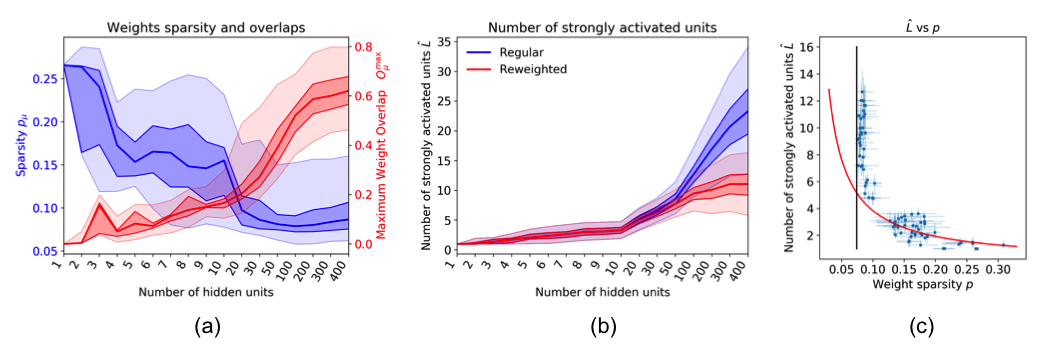
We now study how the value of impacts the representations of the protein sequences. We repeat the training with dReLU RBM fixed regularization for varying between 1 and 400, and show in Fig. 8 one typical weight learnt by dReLU RBMs for varying between 1 and 400. We observe different behaviours, as the value of increases:
For very low , the weight vectors are extended over the whole visible layer. For , the unique weight vector capture electrostatic features – its entries are strong on charged amino acids, such as K, R (positive charges) and E, D (negative charges)–, and is very similar to the top component of the correlation matrix of the data, compare top panel in Fig. 8 and Fig. 4(f). Additional hidden units, see panels on the second line of Fig. 8 corresponding to , capture other collective modes, here patterns of correlated Cystein-Cystein bridges across the protein. Hence, RBM can be seen as a non-linear implementation of Principal Component Analysis. A thorough comparison with PCA will be presented in Section IV.
As increases, the resolution of representations gets finer and finer: units focus on smaller and smaller portions of the visible layer, see Fig. 8. Nonzero entries are restricted to few sites, often in contact on the protein structure, see Fig. 4, fold . We introduce a proxy for the sparsity of the weight based on inverse participation ratios of the entries , see Appendix. The behavior of as a function of is shown in Fig. 9(c). We observe that decreases (weights get sparser) until reaches 50–100.
For values of , the modes of covariation cannot be decomposed into thinner ones anymore, and saturates to the minimal value corresponding to a hidden unit linked to two visible units (Fig. 9(a)). Then, additional features are essentially duplicates of the previous ones. This can be seen from the distribution of maximum weight overlaps shown in Fig. 9(a), see Appendix for definition.
In addition, the number of simultaneously active hidden units per sequence grows, undergoing a continuous transition from a ferromagnetic-like regime () to a compositional one (). Note crucially that does not scale linearly with , see Fig. 9(a,b). If we account for duplicated hidden units, tends to saturate at about , a number that arises from the data distribution rather than from . In contrast, for an unregularized training with quadratic hidden unit potential, grows to much larger values () as increases (Appendix, Fig. S1). Lastly, Fig. 9(c) shows that the theoretical scaling Tubiana and Monasson 2017 is qualitatively correct.

IV Comparison with other Representation Learning Algorithms

IV.1 Models and definitions
We now compare the results obtained with standard representation learning approaches. Thanks to popular packages such as Scikit-learn or Keras, most of these approaches are easy to implement in practice.
Principal Component Analysis (PCA) is arguably the most commonly used tool for finding the main modes of covariation of data. It is routinely applied in the context of protein sequence analysis for finding protein subfamilies, identifying specificity-determining positions Casari et al. 1995; Rausell et al. 2010; De Juan et al. 2013, and defining subsets of sites (called sectors) within proteins that control the various properties of the protein Halabi et al. 2009; McLaughlin Jr et al. 2012. A major drawback of PCA is that it assumes that the weights are orthogonal, which is in general not true and often results in extended modes that cannot be interpreted easily. Independent Component Analysis (ICA) Bell and Sejnowski 1995; Hyvärinen and Oja 2000 is another approach that aims at alleviating this issue by incorporating high-order moments statistics into the model; ICA was applied for identifying neural areas from fMRI data McKeown et al. 1998, and also used for protein sequence analysis Rivoire et al. 2016. Another way to break the rotational invariance is to impose sparsity constraints on the weights or the representation via regularization. Sparse PCA Zou et al. 2006 is one such popular approach, and was considered both in neuroscience Baden et al. 2016 and protein sequence analysis Quadeer et al. 2018. We will also study sparse (in weights) single-layer noisy autoencoders, which can be seen as a nonlinear variant of sparse PCA. Sparse dictionaries Olshausen and Field 1996; Mairal et al. 2009 are also considered. Finally, we will consider Variational Autoencoders Kingma and Welling 2013 with a linear-nonlinear decoder, which can be seen both as regularized autoencoder and as a nonlinear generative PCA. VAE were recently considered for generative purpose in proteins Sinai et al. 2017; Riesselman et al. 2017; Greener et al. 2018, and their encoder defines a representation of the data.
All the above mentioned model belong to the same family, namely of the linear-nonlinear latent variable graphical models, see Fig. 10. In this generative model, latent factors are drawn from an independent distribution , and the data is obtained, as in RBM, by a linear transformation followed by an element-wise nonlinear stochastic or deterministic transformation, of the form . Unlike in RBM, a single pass is sufficient to sample configurations rather than an extensive back-and-forth process. For a general choice of and , the inference of this model by maximum likelihood is intractable because the marginal does not have a closed form. The different models correspond to different hypothesis on , , and learning principles that simplify the inference problem, see Table 1.
| Algorithm | PCA | ICA (Infomax) | Sparse PCA | Sparse noisy | Sparse Dictionaries | Variational |
|---|---|---|---|---|---|---|
| Autoencoders | Autoencoders | |||||
| Gaussian | Non-Gaussian | / | / | Sparse | Gaussian | |
| Deterministic | Deterministic | Deterministic | Deterministic | Deterministic | Stochastic | |
| Deterministic | Deterministic | Deterministic | Stochastic | Deterministic | Stochastic | |
| Linear | Linear | Linear | Softmax | Linear | Softmax | |
| Orthonormal | Normalized | Sparse | Sparse | Normalized | Sparse | |
| Learning | Max. Likelihood | Max. Likelihood | Min. Reconstruction | Min. Noisy | Min. Reconstruction | Variational |
| Method | Min. Reconstruction | Error (MSE) | Reconstruction | Error (MSE) | Max. Likelihood | |
| Error (MSE) | Error (CCE) |
IV.2 Lattice Proteins: Features inferred

We use each approach to infer features from the MSA Lattice Proteins. For each model, we use the same number of latent factors. For PCA, ICA and Sparse Dictionaries, we used one-hot-encoding for each site (i.e. converted into a 20-dimensional binary vector), and the standard implementation from Scikit-learn with default parameters. For sparse dictionaries, we adjusted the penalty such that the number of simultaneously active latent features matches the one found in RBM . Sparse PCA and sparse autoencoders are special cases of autoencoders, respectively with a mean square reconstruction error and categorical cross-entropy reconstruction error, and were implemented in Keras. In both cases we used the same weights for encoding and decoding. For the noisy variant, we replace 20% of the amino acids with a random one before attempting to reconstruct the original sequence. For Variational Autoencoders, we used the same parametric form of as for RBM, i.e. a linear transformation followed by a categorical distribution. The posterior probability is approximated by a Gaussian encoder where and are computed from either by linear transformation or by a single hidden layer neural network; the parameters of both and the encoder are learnt by maximizing the variational lower bound on the likelihood of the model. The sparse regularization is enforced on the ’decoding’ weights of only. For all models with a sparse weight regularization, we selected the regularization strength so as to obtain similar median sparsity values as with the RBM shown in Fig. 5. We show for each method six selected features in Fig. 11 (PCA, sPCA, sNAE, sVAE with linear encoder), and in Appendix Fig. S2 (ICA, Sparse Dictionaries, sVAE with nonlinear encoder). For PCA, ICA and Sparse Dictionaries, we show the most important features in terms of explained variance. For sPCA, sNAE and sVAE, we show features with sparsity close to the median sparsity.
Most of the high importance features inferred by PCA, ICA are completely delocalised and encode the main collective modes of the data, similarly to unregularized RBM. Clearly, there is no simple way to relate these features to the underlying interactions of the system. Even if sparsity could help, the main issue is the enforced constraint of decorrelation/independance, because it impedes the model from inferring smaller coevolutionary modes such as pairs of amino acids in contact. Indeed, Lattice Proteins exhibits a hierarchy of correlations, with sites that are tightly correlated, and also weakly correlated to others. For instance, hidden units 4 and 5 of Fig. 5 are strongly but not completely correlated, with a small fraction of sequences having and and conversely (Appendix Fig. S4(a)). Therefore, neither PCA nor ICA can resolve the modes; instead, the first principal component is roughly the superposition of both modes (Fig. 4(e)). Finally, both PCA and ICA also infer a feature that focuses only on site 24 (PC4 and IC4). As seen from the conservation profile (Fig. 4(d)), this site is strongly conserved, with two possible amino acids. Since mutations are uncorrelated from the remaining of the sequence and the associated variance of the mode is fairly high, both PCA and ICA encode this site. In contrast, we never find a hidden unit focusing only on a single site with RBM, because its effect on is equivalent to a field term. Similar features are found with Sparse Dictionaries as well, see Appendix.
As expected, all the models with sparse weights penalties (sPCA, sNAE and sVAE) can infer localized features, provided the regularization is adjusted accordingly. However, unlike in RBM, a significant fraction of these features does not focus on sites in contact. For instance, in sparse PCA the features 2 and 5 focus respectively on pairs 6-17 and 17-21, and neither of them are in contact. To be more systematic, we identify for each method the features focusing on two and three sites (via the criterion ), count them and compare them to the original structure. Results are shown in Table 2. For RBM, 49 hidden units focus on two sites, of which 47 are in contact, and 18 focus on three sites, of which 16 are in contact (e.g. like 8-16-27). For the other methods, both the number of features and the true positive rate are significantly lower. In Sparse PCA, only 15/25 pairs and 3/24 triplet features are legitimate contacts or triplets in the structure.
| Sparse Model | Pair features | Triplet features |
|---|---|---|
| RBM | 47/49 | 16/18 |
| sPCA | 15/25 | 3/24 |
| Noisy sAE | 20/29 | 7/19 |
| sVAE (linear encoder) | 8/8 | 5/6 |
| sVAE (nonlinear encoder) | 6/6 | 2/4 |
The main reason for this failure is that in sparse PCA (as in PCA), emphasis is put on the complete reconstruction of the sequence from the representation because the mapping is assumed to be deterministic rather than stochastic. The sequence must be compressed entirely in the latent factors, of smaller size , and this is achieved by ‘grouping’ sites in a fashion that may respect some correlations, but not necessarily the underlying interactions. Therefore, even changing the reconstruction error to cross-entropy to properly take into account the categorical nature of the data does not significantly improve the results. However, we found that corrupting the sequence with noise before attempting to reconstruct it (i.e. introducing a stochastic mapping) indeed slightly improves the performance, though not to the same level as RBM for quantitative modeling.
The simplifying assumption that is deterministic can be lifted by adopting a variational approach for learning the model; in the case of Gaussian distribution for we obtain the Variational Autoencoder model. The features obtained are quite similar to the ones obtained with RBM, featuring contacts, triplets (with very few false positives) and some extended modes. Owing to this stochastic mapping, the representation need not encode individual site variability, and focuses instead on the collective behavior of the system.
The major inconvenient of VAE is that we find that only a small number of latent factors () are effectively connected to the visible layer. Increasing the number of latent factors or changing the training algorithm (SGD vs ADAM, Batch Normalization) did not improve this number. This is likely because the independent Gaussian assumption is not compatible with the linear-nonlinear decoder and sparse weights assumption. Indeed, the posterior distribution of the latent factors (from ) show significant correlations and deviations from Gaussianity (Appendix Fig. S4(b,c)); The KL regularization term of VAE training therefore encourages them from being disconnected. Another consequence of this deviation from i.i.d. Gaussian is that sequences generated with the VAE have significantly lower fitness and diversity than with RBM (Appendix Figs. S5,S6). Though deep mappings between the representation and the sequence (as in Riesselman et al. 2017), as well as more elaborate priors (as in Mescheder et al. 2017) can be considered for quantitative modeling , the resulting models are significantly less interpretable. In contrast, undirected graphical models such as RBM have a more flexible latent variable distribution, and are therefore more expressive for a fixed linear-nonlinear architecture.
In summary, the key ingredients allowing to learn RBM-like representations are i) Sparse weights ii) Stochastic mapping between configurations and representations and iii) Flexible latent variable distributions.
IV.3 Lattice Proteins: Robustness of features
Somewhat surprisingly, we also find that allowing a stochastic mapping between representation and configurations results in features that are significantly more robust with respect to finite sampling. For all the models and parameters used above, we repeat the training five times with either the original data set and varying seed or the shuffled data set, in which each column is shuffled independently from the others so as to preserve the first order moments and to suppress correlations. For a sample of very large size, the models trained on the shuffled data should have latent factors that are either disconnected or localized on a single site, with small feature importance. We show in Fig. 12 and Appendix Fig. S7 the distribution of feature importance for the original and shuffled data, for each method. For PCA, ICA, sparse PCA and sparse autoencoders, the weights are normalized and feature importance is determined by the variance of the corresponding latent factor. For RBM and VAE, the variance of the latent factors is normalized to 1 and the importance is determined by the weight amplitude. In PCA and ICA, we find that only a handful of features emerge from the bulk; sparse regularization slightly improves the number but not by much. In contrast, there is a clean scale separation between feature importance for regular and shuffled data, for both regularized and unregularized RBM and VAE. This notably explains why only few principal components can be used for protein sequence modelling, whereas many features can be extracted with RBM. The number of modules that can be distinguished within protein sequences is therefore grossly underestimated by Principal Component Analysis.

V Conclusion
Understanding the collective behavior of a physical system from observations requires to learn a phenomenology of data, as well as to infer the main interactions that drive its collective behavior. Representation learning approaches, such as as Principal Component Analysis or Independent Component Analysis have been frequently considered for this purpose. Comparatively, Restricted Boltzmann Machines, a Machine Learning tool originally popularized for unsupervised pretraining of Deep Neural Networks have received little attention, notably due to a limited of understanding of the properties of the learnt representations.
In this work, we have studied in detail the performances of RBM on a notoriously difficult problem, that is, the prediction of the properties of proteins from their sequence (the so-called genotype-to-phenotype relationship). We have shown that, provided that appropriate non-quadratic potentials, as well as sparsity regularization over the weights are used, RBM can learn compositional representations of data, in which the hidden units code for constitutive parts of the data configurations. Each constitutive part, due to sparsity, focuses on a small region of the data configurations (subset of visible sites), and is therefore easier to interpret that extended features. Constitutive parts may, in turn, be stochastically recombined to generate new data with good properties (here, probability of folding into the desired 3D structure). Regularized RBM therefore offer an appealing compromise between model interpretability and generative performance.
We stress that the behavior of RBM described above is in full agreement with theoretical studies of RBM with weights extracted from random statistical ensembles, controlled by a few parameters, including the sparsity, the aspect ratio of the machine, the thresholds of rectified linear units Tubiana and Monasson 2017. It is however a non trivial result, due to the very nature of the lattice-protein sequence distribution, that forcing RBM trained on such data to operate in the compositional regime can be done at essentially no cost in log-likelihood (see Fig. 7(b)). This property also holds for real proteins, as shown in Tubiana et al. 2018.
In addition, RBM enjoys some useful properties with respect to the other representation learning approaches studied in the present work. First, RBM representations focus on the underlying interactions between components rather than on all the variability of the data, taken into account by site-dependent potentials acting on the visible unit. The inferred weights are therefore fully informative on the key interactions within the system. Secondly, the distribution of latent factors (Fig. 10) is not imposed in RBM, contrary to VAE where it is arbitrarily supposed to be Gaussian. The inference of the hidden-unit potential parameters (thresholds and curvatures for dReLU units) confers a lot of adaptibility to RBM to fit as closely as possible the data distribution.
Altogether, beyond the protein sequence analysis application presented here, our work suggests that RBM shed a different light on data and could find usage to model other data in an accurate and interpretable way. It would be very interesting to extend this approach to deeper architectures, and see how the nature of representations vary from layer to layer. Another possible extension regards sampling. RBM, when driven in the compositional phase, empirically show efficient mixing properties. Characterizing how fast the data distribution is dynamically sampled would be very interesting, with potential payoff for training where benefiting from efficient sampling is crucial.
Acknowledgments
We acknowledge Clément Roussel for helpful comments. This work was partly funded by the ANR project RBMPro CE30-0021-01. J.T. acknowledges funding from the Safra Center for Bioinformatics, Tel Aviv University.
References
- Schwarz et al. (2014) D. A. Schwarz, M. A. Lebedev, T. L. Hanson, D. F. Dimitrov, G. Lehew, J. Meloy, S. Rajangam, V. Subramanian, P. J. Ifft, Z. Li, et al., Nature methods 11, 670 (2014).
- Wolf et al. (2015) S. Wolf, W. Supatto, G. Debrégeas, P. Mahou, S. G. Kruglik, J.-M. Sintes, E. Beaurepaire, and R. Candelier, Nature methods 12, 379 (2015).
- Finn et al. (2015) R. D. Finn, P. Coggill, R. Y. Eberhardt, S. R. Eddy, J. Mistry, A. L. Mitchell, S. C. Potter, M. Punta, M. Qureshi, A. Sangrador-Vegas, et al., Nucleic acids research 44, D279 (2015).
- Kolodziejczyk et al. (2015) A. A. Kolodziejczyk, J. K. Kim, V. Svensson, J. C. Marioni, and S. A. Teichmann, Molecular cell 58, 610 (2015).
- Fowler et al. (2010) D. M. Fowler, C. L. Araya, S. J. Fleishman, E. H. Kellogg, J. J. Stephany, D. Baker, and S. Fields, Nature methods 7, 741 (2010).
- McKeown et al. (1998) M. J. McKeown, S. Makeig, G. G. Brown, T.-P. Jung, S. S. Kindermann, A. J. Bell, and T. J. Sejnowski, Human brain mapping 6, 160 (1998).
- Rivoire et al. (2016) O. Rivoire, K. A. Reynolds, and R. Ranganathan, PLoS computational biology 12, e1004817 (2016).
- Nguyen et al. (2017) H. C. Nguyen, R. Zecchina, and J. Berg, Advances in Physics 66, 197 (2017).
- Cocco et al. (2018) S. Cocco, C. Feinauer, M. Figliuzzi, R. Monasson, and M. Weigt, Reports on Progress in Physics 81, 032601 (2018).
- Weigt et al. (2009) M. Weigt, R. A. White, H. Szurmant, J. A. Hoch, and T. Hwa, Proceedings of the National Academy of Sciences 106, 67 (2009).
- Morcos et al. (2011) F. Morcos, A. Pagnani, B. Lunt, A. Bertolino, D. S. Marks, C. Sander, R. Zecchina, J. N. Onuchic, T. Hwa, and M. Weigt, Proceedings of the National Academy of Sciences 108, E1293 (2011).
- Figliuzzi et al. (2016) M. Figliuzzi, H. Jacquier, A. Schug, O. Tenaillon, and M. Weigt, Molecular Biology and Evolution 33, 268 (2016).
- Hopf et al. (2017) T. A. Hopf, J. B. Ingraham, F. J. Poelwijk, C. P. Schärfe, M. Springer, C. Sander, and D. Marks, Nature Biotechnology 35, 128 (2017).
- Tkacik et al. (2010) G. Tkacik, J. S. Prentice, V. Balasubramanian, and E. Schneidman, Proceedings of the National Academy of Sciences USA 107, 14419 (2010).
- Posani et al. (2017) L. Posani, S. Cocco, K. Ježek, and R. Monasson, Journal of computational neuroscience 43, 17 (2017).
- Ackley et al. (1987) D. H. Ackley, G. E. Hinton, and T. J. Sejnowski, in Readings in Computer Vision (Elsevier, 1987) pp. 522–533.
- Hinton (2002) G. E. Hinton, Neural computation 14, 1771 (2002).
- Hinton et al. (2006) G. E. Hinton, S. Osindero, and Y.-W. Teh, Neural computation 18, 1527 (2006).
- Tubiana et al. (2018) J. Tubiana, S. Cocco, and R. Monasson, arXiv preprint arXiv:1803.08718 (2018).
- Tubiana and Monasson (2017) J. Tubiana and R. Monasson, Physical review letters 118, 138301 (2017).
- Barra et al. (2012) A. Barra, A. Bernacchia, E. Santucci, and P. Contucci, Neural Networks 34, 1 (2012).
- Tieleman (2008) T. Tieleman, in Proceedings of the 25th international conference on Machine learning (ACM, 2008) pp. 1064–1071.
- Desjardins et al. (2010a) G. Desjardins, A. Courville, Y. Bengio, P. Vincent, and O. Delalleau, in Proceedings of the thirteenth international conference on artificial intelligence and statistics (2010) pp. 145–152.
- Desjardins et al. (2010b) G. Desjardins, A. Courville, and Y. Bengio, arXiv preprint arXiv:1012.3476 (2010b).
- Salakhutdinov (2010) R. Salakhutdinov, in Proceedings of the 27th International Conference on Machine Learning (ICML-10) (2010) pp. 943–950.
- Cho et al. (2010) K. Cho, T. Raiko, and A. Ilin, in Neural Networks (IJCNN), The 2010 International Joint Conference on (IEEE, 2010) pp. 1–8.
- Gabrié et al. (2015) M. Gabrié, E. W. Tramel, and F. Krzakala, in Advances in Neural Information Processing Systems (2015) pp. 640–648.
- Tramel et al. (2017) E. W. Tramel, M. Gabrié, A. Manoel, F. Caltagirone, and F. Krzakala, arXiv preprint arXiv:1702.03260 (2017).
- Hyvärinen and Oja (2000) A. Hyvärinen and E. Oja, Neural networks 13, 411 (2000).
- Fischer and Igel (2012) A. Fischer and C. Igel, in Iberoamerican Congress on Pattern Recognition (Springer, 2012) pp. 14–36.
- (31) One extreme example of such intricate representation is the random gaussian projection for compressed sensing donoho2006compressed. Provided that the configuration is sparse in some known basis, it can be reconstructed from a small set of linear projections onto random iid gaussian weights . Although such representation carries all information necessary to reconstruct the signal, it is by construction unrelated to the main statistical features of the data.
- Olshausen and Field (1996) B. A. Olshausen and D. J. Field, Nature 381, 607 (1996).
- Mairal et al. (2009) J. Mairal, F. Bach, J. Ponce, and G. Sapiro, in Proceedings of the 26th annual international conference on machine learning (ACM, 2009) pp. 689–696.
- Agliari et al. (2012) E. Agliari, A. Barra, A. Galluzzi, F. Guerra, and F. Moauro, Phys. Rev. Lett. 109, 268101 (2012).
- Amit et al. (1985) D. J. Amit, H. Gutfreund, and H. Sompolinsky, Physical Review Letters 55, 1530 (1985).
- Shakhnovich and Gutin (1990) E. Shakhnovich and A. Gutin, The Journal of Chemical Physics 93, 5967 (1990).
- Jacquin et al. (2016) H. Jacquin, A. Gilson, E. Shakhnovich, S. Cocco, and R. Monasson, PLoS computational biology 12, e1004889 (2016).
- Miyazawa and Jernigan (1996) S. Miyazawa and R. L. Jernigan, Journal of molecular biology 256, 623 (1996).
- Neal (2001) R. M. Neal, Statistics and computing 11, 125 (2001).
- Salakhutdinov and Murray (2008) R. Salakhutdinov and I. Murray, in Proceedings of the 25th international conference on Machine learning (ACM, 2008) pp. 872–879.
- Casari et al. (1995) G. Casari, C. Sander, and A. Valencia, Nature Structural and Molecular Biology 2, 171 (1995).
- Rausell et al. (2010) A. Rausell, D. Juan, F. Pazos, and A. Valencia, Proceedings of the National Academy of Sciences 107, 1995 (2010).
- De Juan et al. (2013) D. De Juan, F. Pazos, and A. Valencia, Nature Reviews Genetics 14, 249 (2013).
- Halabi et al. (2009) N. Halabi, O. Rivoire, S. Leibler, and R. Ranganathan, Cell 138, 774 (2009).
- McLaughlin Jr et al. (2012) R. N. McLaughlin Jr, F. J. Poelwijk, A. Raman, W. S. Gosal, and R. Ranganathan, Nature 491, 138 (2012).
- Bell and Sejnowski (1995) A. J. Bell and T. J. Sejnowski, Neural computation 7, 1129 (1995).
- Zou et al. (2006) H. Zou, T. Hastie, and R. Tibshirani, Journal of computational and graphical statistics 15, 265 (2006).
- Baden et al. (2016) T. Baden, P. Berens, K. Franke, M. R. Rosón, M. Bethge, and T. Euler, Nature 529, 345 (2016).
- Quadeer et al. (2018) A. A. Quadeer, D. Morales-Jimenez, and M. R. McKay, bioRxiv , 307033 (2018).
- Kingma and Welling (2013) D. P. Kingma and M. Welling, arXiv preprint arXiv:1312.6114 (2013).
- Sinai et al. (2017) S. Sinai, E. Kelsic, G. M. Church, and M. A. Novak, arxiv:1712.03346 (2017).
- Riesselman et al. (2017) A. J. Riesselman, J. B. Ingraham, and D. S. Marks, arxiv:1712.06527 (2017).
- Greener et al. (2018) J. G. Greener, L. Moffat, and D. T. Jones, Scientific reports 8, 16189 (2018).
- Mescheder et al. (2017) L. Mescheder, S. Nowozin, and A. Geiger, arXiv preprint arXiv:1701.04722 (2017).
Annex: Proxies for weight sparsity, number of strongly activated hidden units
Since neither the hidden layer activity nor the weights are exactly zero, proxies are required for evaluating them. In order to avoid the use of arbitrary thresholds which may not be adapted to every case, we use Participation Ratios.
The Participation Ratio of a vector is:
| (21) |
If has nonzero and equal (in modulus) components PR is equal to for any . In practice we use the values and 3: the higher is, the more small components are discounted against strong components in . Note also that it is invariant to rescaling of .
PR can be used to estimate the weight sparsity for a given hidden unit, and averaged to get a single value for a RBM.
| (22) |
Similarly, the number of strongly activated hidden units for a given visible layer configuration can be computed with a participation ratio. For non-negative hidden units such as with the ReLU potential, it is obtained via:
| (23) |
For dReLU hidden units, which can take both positive and negative values and may have e.g. bimodal activity, their most frequent activity can be non-zero. We therefore subtract it before computing the participation ratio:
| (24) |
To measure the overlap between hidden units , we introduce the quantities
| (25) |
which takes values in the range. We also define .
To account for strongly overlapping hidden units, one can also compute the following weighted participation ratio:
| (26) |
where is chosen as the inverse of the number of neighboring hidden units, defined according to the criterion . This way, two hidden units with identical weights contribute to the participation ratio as much as a single isolated one.
Annex: Supplementary figures


