Phase Transitions in Nematics: Textures with Tactoids and Disclinations
Abstract
We demonstrate that a first order isotropic-to-nematic phase transition in liquid crystals can be succesfully modeled within the generalized Landau-de Gennes theory by selecting an appropriate combination of elastic constants. The numerical simulations of the model established in this paper qualitatively reproduce the experimentally observed configurations that include interfaces and topological defects in the nematic phase.
keywords
uniaxial nematic, isotropic, Landau-de Gennes, tactoid, disclination, phase transition1 Introduction
Phase transitions between ordered and isotropic states in nematic liquid crystals are of interest both for technological reasons as well as because nematics offer one of the simplest experimental systems where interfaces and topological defects may coexist. In particular, a uniaxial nematic liquid crystal typically consists of asymmetrically-shaped molecules that under appropriate conditions tend to align roughly in the same direction. The preferred molecular orientation in a given region occupied by a uniaxial nematic is often described in terms of the unit vector field , called the director. A more precise description takes into account the non-polar character of ordering, e.g., because the probabilities of finding the head or the tail of a molecule in a given direction are equal. This description replaces the director with a projection matrix which can be identified with an element of the projective space and is invariant with respect to reversal of orientation .
Two different types of topological defects can be present in a nematic in three dimensions: -dimensional point defects also known as vortices or nematic hedgehogs and -dimensional disclinations. Point defects may also be present on the surface of a nematic; such defects are known as boojums. There is a large body of literature devoted to the study of nematic defects and we refer the reader to [1] for a comprehensive exposition on the topic. Our principal interest in this work is to examine the interaction between the nematic defects and isotropic-to-nematic interfaces.
The interfaces form in the process of the first order isotropic-to-nematic phase transition that can be induced either by lowering temperature (thermotropic nematics) or increasing the concentration of asymmetric molecules in a solvent (lyotropic nematics). Typically, nuclei of the nematic phase form within the isotropic phase upon lowering the temperature. The nematic nuclei are separated from the isotropic regions by phase boundaries or interfaces. The interfaces subsequently propagate converting the isotropic phase to the nematic phase in the process. In addition to motion of interfaces, the resulting dynamics of the system involves formation, annihilation and propagation of various types of defects.
In a recent work [2], the authors examine the interplay between the interfaces and defects that are present during phase transitions in lyotropic chromonic liquid crystals (LCLC). The principal feature of the isotropic-to-nematic phase transition in LCLC is that the interface provides an “easy direction” for nematic anchoring on the interface which in this case forces the director field to be tangent to this phase boundary. When combined with the anchoring (boundary) conditions on the walls of the container, the topology of the nematic configuration leads to formation of structural defects.
Our goal in the present paper is to demonstrate that the zoo of singularities observed in [2] can be described within the framework of the Landau-de Gennes model for -tensors related to the projection matrix descriptor of the nematic phase alluded to above. Critical to our modeling will be an assumption of large disparity between the values of the elastic constants appearing in the energy. In Section 2 we briefly describe the experimental observations that expand on some of the results presented in [2] by incorporating scenarios of the phase transition in which the isotropic phase regions, often called “negative tactoids” [3], [2], or simply “tactoids”, shrink into a uniform nematic state or a state with a topological defect, depending on the winding number of the tactoid. Note here that positive tactoids, i.e., regions of a nematic surrounded by an isotropic melt, have been previously theoretically treated in [4]-[9].
2 Experimental Results
The sample configuration consisted of the ITO glass that was spin-coated with a polyimide layer, SE7511, in which the directors of disodium chromoglycate (DSCG) are aligned parallel to substrates. Subsequently, two substrates were assembled into a cell with the thickness of 2 m. wt% of DSCG solution was injected into the assembled cell.
The cell was cooled at the rate of . As the temperature decreased from the isotropic phase, nematic domains appeared, grew, and coalesced. When many large nematic domains coalesced, they occasionally trapped isotropic islands, or tactoids, around which the director may have either zero or nonzero winding number. The snapshots of configurations with islands having different winding number of the director on their boundary are shown in Figs. 1-2. These are Polscope textures with color representing optical retardance, bars giving the orientation of the director, and circles indicating the point where orientation was measured.


3 Landau-de Gennes Model
3.1 The -tensor
Given a point , the second moment of the orientational distribution of the rod-like nematic liquid crystal molecules near can be described by a -tensor that takes the form of a symmetric, traceless matrix. By virtue of being symmetric and traceless, has three real eigenvalues and that satisfy
and a mutually orthonormal eigenframe . While a more detailed overview of the theory can be found in [10], below we outline the key elements that will be needed in the developments below.
Suppose that Then the liquid crystal is in a uniaxial nematic state and
| (1) |
where is the uniaxial nematic order parameter and is the nematic director. If there are no repeated eigenvalues, the liquid crystal is said to be in a biaxial nematic state, while it is in the isotropic state when all three eigenvalues and hence itself vanish. The isotropic state of a liquid crystal is associated, for instance, with a high temperature regime.
3.2 Landau-de Gennes energy
Suppose that the bulk elastic energy density of a nematic liquid crystal is given by a frame-indifferent expression . A common expression that includes terms up to the second order in reads
| (3) |
The bulk Landau-de Gennes energy density is
| (4) |
cf. [10]. Here is the -th column of the matrix and is the dot product of two matrices Further, the coefficient is temperature-dependent and in particular is negative for sufficiently low temperatures. One readily checks that the form (4) of this potential implies that in fact depends only on the eigenvalues of , and due to the trace-free condition, therefore depends only on two eigenvalues. The form of guarantees that the isotropic state yields a global minimum at high temperatures while a uniaxial state of the form (1) gives the minimum when temperature (i.e. the parameter ) is reduced below a certain critical value, cf. [13, 10]. We remark for future use that is bounded from below and can be made non-negative by adding an appropriate constant.
We now turn to the behavior of the nematic on the boundary of the sample. Here two alternatives are possible. First, the Dirichlet boundary conditions on are referred to as strong anchoring conditions in the physics literature: they impose specific preferred orientations on nematic molecules on surfaces bounding the liquid crystal. An alternative is to specify the anchoring energy on the boundary of the sample; then orientations of the molecules on the boundary are determined as a part of the minimization procedure. This approach is known as weak anchoring.
4 Model Development
In this section we derive a version of the Landau-de Gennes model that is appropriate for the modeling of nematic systems with disparate elastic constants. In particular, we are interested in the case when the elastic constant corresponding to splay deformations is larger than those for bend and twist so that the splay of the director is relatively expensive. Note that this situation can be found in experimental systems, such as chromonic lyotropic liquid crystals [14] shown in Figures 1-2 and in thermotropic nematics of certain molecular shape, such as dimers [15]. To this end, let
and consider the Landau-de Gennes potential defined in eq. 4. As long as , one finds that this potential depends only on the eigenvalues of , say and with , and with a slight abuse of notation we arrive at
We are interested in describing the extrema of . Taking the derivatives of gives
It is easy to check that the critical points of are as well as , , and , where solves
| (6) |
The point corresponds to a local minimum of if and to a local maximum of if . The solutions of eq. 6 are given by
hence there are no nematic critical points whenever and has a single extremum corresponding to the global minimum at . By considering second derivatives of , we also find that
| (7) |
is a point of a local minimum and
is a saddle point of if . We conclude that the nematic minima at , , and coexist with the isotropic minimum at as long as . An easy computation shows that all of these minima have the same depth of when
| (8) |
Because here we will be interested in the regime when the energy value in the isotropic state is greater than or equal to the minimum energy in a nematic state, we subtract
| (9) |
from to ensure that the global minimum value of the Landau-de Gennes energy is . Hence, from now on
Note that decreasing from to corresponds to increased undercooling and a larger thermodynamic force driving the isotropic-to-nematic phase transition.
Let denote the region occupied by the liquid crystal sample. To derive an expression for the elastic energy, recall first that the Oseen-Frank energy defined over director fields is given by
where for simplicity we assume that the admissible competitors are subject to the same Dirichlet boundary data on . Assuming in this paper that , the energy can be written (up to null Lagrangian terms) as
| (10) |
where and are nonnegative elastic constants. We want to derive a well-posed variational problem for -valued fields such that the elastic energy for formally reduces to eq. 10 whenever is in a nematic state that minimizes the potential energy . To this end, the minimum of is achieved whenever has eigenvalues , , and so that can be written as
where is a unit eigenvector corresponding to the eigenvalue . From this equation,
and it can be easily checked that
while
Making use of the fact that
it follows that
and
where and . Note that here we switched the indices of the elastic constants in order to conform with the standard notation (cf. eq. 3).
The total energy of a nematic configuration as described within the Landau-de Gennes -tensor theory in this work will be given by
| (11) |
where is a constant that has units of energy per unit volume.
Remark 1.
Now let denote a characteristic length of the problem and set
Before proceeding further, we introduce the following rescalings
| (12) |
and drop the bar notation to obtain
| (13) |
where
| (14) |
In this scaling, the potential given by (14) is now minimized by any symmetric traceless matrix with eigenvalues , and the global minimum value of is equal to zero.
In our simulations we consider a simplified form of a -tensor that can be obtained via a dimension reduction procedure for thin nematic films [17]. In the corresponding ansatz, one eigenvector of admissible -tensors must be perpendicular to the plane of the film. Then in the system of coordinates in which the normal to the film is parallel to the -axis, the -tensor is independent of and can be written [18] as
| (15) |
for a scalar-valued function and vector-valued function . Let
so that
where is the identity matrix. In terms of and the contributions to the energy density are as follows
and
Suppose that the film occupies the region . The system of Euler-Lagrange PDEs corresponding to the energy functional eq. 13 then takes the form
| (16) |
| (17) |
| (18) |
where
are the Pauli matrices.
When the liquid crystal is in the energy minimizing nematic state while the director lies in the plane of the film, we have
It follows from this computation that
| (19) |
hence the vector winds twice as fast along a given curve in , compared to the director when is planar.
More generally, the ansatz eq. 15 splits the nematic component of the minimal set of the bulk energy into two disconnected components
and
Here the first component corresponds to a constant nematic state with the director perpendicular to the surface of the film. The second component includes all configurations with the director lying in the plane of the film—these configurations can be nontrivial and, in particular, they include the director fields that carry a nonzero winding number.
Since we are interested in regimes when both nematic and isotropic phases coexist, we recall that whenever
the set
yields a local minimum of corresponding to the isotropic phase. The corresponding local minimum energy value is greater than or equal to the global minimum value of . When , the set
gives the third connected component of the minimal set of the bulk energy.
Given that has a multi-component minimal set, the energy eq. 13 is of Allen-Cahn-type as long as the factor in front of is large. To this end, in what follows we assume that and is small. We will consider gradient flow dynamics associated with this model, but before we proceed further it is worth comparing our present situation to the more familiar one of gradient flow dynamics for a multi-well Allen-Cahn type potential with diffusion given simply by the Laplacian. In this scaling, when the diffusion is given by the Laplacian, formal asymptotics suggest that for Allen-Cahn dynamics one should expect an interface propagating by curvature flow that separates the different phases defined by components of the zero set of the potential. In the scalar setting of Allen-Cahn where a double well potential vanishes at two points, there are by now numerous rigorous proofs of this fact based on maximum principles, barriers and/or comparison principles, see e.g. [19, 20, 21, 22] as well as the energetic argument in the radial setting in [23]. For the vector setting of time-dependent Allen-Cahn, formal asymptotics based on multiple time-scale expansions again suggest that mean curvature flow emerges as the governing equation for the interface, [24, 25].
What distinguishes the dynamics in the present study, however, is the anisotropy of the diffusive terms indicated by the presence of the divergence terms in (16)–(18). While we again anticipate that in the regime an interface separating the different phases of the tensor will evolve by a law involving curvature, the process will be significantly affected by the interaction between the director associated with and the normal to the interface.
Our present model is closely related to the investigation in [26] of the asymptotics for a director-like model based on an -valued order parameter . There the elastic energy is similarly anisotropic and is coupled to a Chern-Simons-Higgs-type potential . Thus, the structure of the energy functional in [26] is similar to the setup proposed here in that it involves a potential with minima at the isotropic and a nematic state as well as the elastic terms that are quadratic in the gradient of the order parameter field. The term penalizing splay deformations in [26] dominates other elastic terms so that the divergence of the director is very expensive. The principal difference between the model considered in [26], which from now on we will refer to as the CSH-director model, and the present work is that here we consider non-orientable tensor fields, while the admissible fields in [26] are orientable.
Our numerical results indicate that similarity between the models leads to similar properties of critical points. In particular, one of the principal observations in [26] is that the director field is parallel to the interface in its immediate vicinity when the parameter is small. The same behavior is exhibited by the numerically obtained critical points of the Landau-de Gennes energy eq. 11, as will be demonstrated in the next section.
We introduce dynamics into the problem by assuming that evolution of the isotropic-to-nematic transition proceeds via gradient flow
where and are inverses of the scalar mobilities of and , respectively. This gives the following systems of PDEs
| (20) |
| (21) |
| (22) |
In order to simulate experimentally available configurations, we will set the initial configuration of to consist of an isotropic region embedded in a nematic phase corresponding to the component of the minimal set of . That is, we will assume that the initial condition is an appropriate mollification of such that
| (23) |
Here is the characteristic function of the region occupied by the nematic phase. We also impose boundary conditions on with values in ; we will assume that the boundary data for may have a nonzero winding number.
In the next section we present the result of simulations for the system eq. 20-eq. 22 and compare the numerical outcomes to experimental observations. We remind the reader that our goal in the present paper is to demonstrate numerically that behavior of interfaces and singularities observed in experiments with chromonic liquid crystals can be qualitatively recovered within the framework of the Landau-de Gennes model. We leave for future work both formal and rigorous analysis of our results, as well as any quantitative considerations and associated modifications of the model.
5 Simulations vs Experiment
The simulations in this section are performed using COMSOL Multiphysics® [27] with the domain taken to be a disk of nondimensional radius , centered at the origin. In what follows, we set dimensional and let . The initial data in all simulations is specified by choosing in eq. 23. Both here and below are polar coordinates of the point .
Recall that when and are related via eq. 8 (either in dimensional or nondimensional setting), the energies of the nematic and isotropic states are the same. Then, if in dimensional variables we set
the parameter measures the degree of undercooling in the system. That is, when increases, the bulk energy density of the isotropic state grows with respect to that of the nematic state and thermodynamic forces driving the isotropic-to-nematic transition become stronger. Setting and dropping the bar, the nondimensional and are given by
| (24) |
First, we verify the conjecture that the behavior of interfaces in our Landau-de Gennes system of PDEs with highly anisotropic elastic constants resembles that of interfaces in the related CSH-director system of [26]. To this end, we assume that is given by eq. 8 so that and both the nematic and the isotropic states are the global minimum of the Landau-de Gennes potential . We simulate the system eq. 20-eq. 22 subject to the boundary conditions
Taking into account eq. 19, the director field on the boundary can be chosen as
where the topological degree of is equal to on .
The results of the gradient flow simulation for the degree boundary data are shown in Fig. 3. An initially circular interface is seen to evolve into the shape given in the figure by a thick red curve that is also a contour line of .
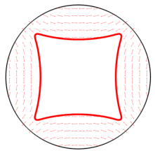
The system in Fig. 3 has reached a steady state that is very similar to what is observed for the CSH-director model in [26]. Indeed, for small , the energy of the isotropic/nematic configuration in both cases should include a penalty for divergence of the director in the nematic phase, as well as the cost for the perimeter of the interface. The anisotropy of the elastic constants also forces the director to align with the interface. The resulting director configuration and the shape of the interface are coupled; in particular, unlike the standard curvature flow, shrinking the perimeter and, thus, size of the isotropic region leads to unbounded growth of the elastic energy. The competition between the perimeter and elastic energy contributions enforces the equilibrium between the two phases observed in Fig. 3.
One is then tempted to ask whether there is any difference between the Landau-de Gennes and the CSH-director model [26] in terms of how the director field extracted from solutions of these two models should behave as . We expect that the difference would manifest itself when the size of an isotropic region is small enough so that this region can be thought of as a core of a topological vortex.
Suppose, for example, that the interface is a single smooth closed curve. Due to the director tangency condition on the interface and because the director field is orientable, the director has the winding number around the interface. When the island shrinks to a small size and because the director is -valued in the nematic phase, topological constraints would keep the isotropic island from disappearing completely in order to prevent the nematic configuration from having an infinite energy. The resulting degree vortex is stable in the CSH-director setting and would persist for a finite time, perhaps until it annihilates with another vortex of the opposite sign or collides with the boundary of .
Now recall that within the Landau-de Gennes theory, a nematic state is described by a -tensor that is a translation and dilation of a projection matrix . The field is not orientable and can be associated with an element of a projective plane . In other words, by working with instead of , we identify the opposite directions and as being the same. As the result, the smallest “quantum” of the winding number for a nematic tensor is . Hence the degree vortex in the director description contains two “quanta” of degree if we switch to the Landau-de Gennes framework. It is a well-established fact that a higher degree vortex is unstable with respect to splitting into several vortices of smaller degrees since the energetic cost of a degree vortex is proportional to , [28]. We expect that the degree CSH vortex would split into two degree vortices when considered in the sense of Landau-de Gennes. Our experimental observations conform to the latter picture; hence the description that disposes with orientability is necessary when considering an isotropic-to-nematic phase transition problem.
We now conduct numerical experiments to test whether evolution of tactoids observed in physical experiments can be captured within the Landau-de Gennes model.
5.1 Degree tactoid
Here we suppose that the director is parallel to the boundary of the disk , e.g.,
so that the topological degree of the orientable director field is equal on . In the non-orientable, -tensor setting the corresponding condition can be expressed as
If the simulations are conducted at zero undercooling, when is given by eq. 8, we observed both here and for the Ginzburg-Landau-type model [26] that, similar to Fig. 3, the isotropic domain evolving via gradient flow shrinks down to a certain size and then stabilizes. In order to drive this size down, we enforce larger undercooling by choosing
The evolution of the nematic/isotropic interface is shown in Fig. 4.


While the isotropic tactoid is not too small, it maintains its circular shape and the director in the nematic region remains parallel to the boundary. Indeed, in this configuration the divergence contribution vanishes, the director is parallel to the interface, and the perimeter of the isotropic tactoid is minimal given its shape.
5.2 Degree tactoid
We now return to the boundary conditions
considered in the beginning of this section for zero undercooling. Here we assume instead that and look for the effects on evolution of the bias between the values of local minima of the potential energy corresponding to the nematic and isotropic state. This bias is associated with lowering the temperature below that of the nematic-to-isotropic transition. The corresponding numerical results are shown in Fig. 5.


The first three figures essentially demonstrate the development of a configuration shown in Fig. 4. The larger thermodynamic forces driving the phase transition in the present case, however, push the size of the tactoid further down essentially to that of a vortex core. At this point, the isotropic region loses stability and splits into two vortices of degree , similar to what can be seen in Fig. 1.
5.3 Degree tactoid
Next, we impose the constant boundary conditions
and suppose that . The numerically computed evolution of a degree zero tactoid that results is shown in Fig. 6 and qualitatively resembles the behavior of a similar tactoid in the experiment as depicted in Fig. 2.


A similar shape is also seen in evolution of degree zero interfaces in the CSH-director model in [26] and is explained by the fact that the director has to be parallel to the interface. In particular, the interface cannot be smooth, for if it were, then it would carry a nonzero topological degree different from the degree on the boundary of the domain.


One interesting issue that we observed in the course of our simulations is illustrated in Fig. 7. When the undercooling is large (), the director appears to be orthogonal to the moving interface rather than being parallel to it as would be expected. A possible explanation for this effect is that the velocity of the interface is relatively large for larger undercoolings and the mobility of the director might not be sufficient for it to relax in a proper direction. We plan to investigate this behavior further in a future work.
5.4 Coalescence of Nematic Tactoids
Finally, the Landau - de Gennes model can also be used to simulate the reverse situation when positive nematic tactoids nucleate in the isotropic phase, then grow and coalesce to form the nematic phase with embedded topological defects (cf. [2]). In Fig. 8 the simulations were conducted subject to Neumann boundary data on and assuming that has radius , while . Three circular tactoids of different orientations were assumed to be present at the time ; in the course of the simulation, tactoids merged generating a single degree defect. This situation closely resembles the original Kibble’s model of strings formed in early universe through coalescence of domains with different “phase” [29].


6 Acknowledgements
DG acknowledges the support from DMREF NSF
DMS-1729538. OL acknowledges the support from DMREF NSF DMS-1729509. PS acknowledges the support from the Simons Collaboration grant 585520.
References
- [1] M. Kleman and O. D. Laverntovich, Soft matter physics: an introduction. Springer Science & Business Media, 2007.
- [2] Y.-K. Kim, S. V. Shiyanovskii, and O. D. Lavrentovich, “Morphogenesis of defects and tactoids during isotropic–nematic phase transition in self-assembled lyotropic chromonic liquid crystals,” Journal of Physics: Condensed Matter, vol. 25, p. 404202, sep 2013.
- [3] Y. A. Nastishin, H. Liu, T. Schneider, V. Nazarenko, R. Vasyuta, S. V. Shiyanovskii, and O. D. Lavrentovich, “Optical characterization of the nematic lyotropic chromonic liquid crystals: Light absorption, birefringence, and scalar order parameter,” Phys. Rev. E, vol. 72, p. 041711, Oct 2005.
- [4] A. Kaznacheev, M. Bogdanov, and A. Sonin, “The influence of anchoring energy on the prolate shape of tactoids in lyotropic inorganic liquid crystals,” Journal of Experimental and Theoretical Physics, vol. 97, no. 6, pp. 1159–1167, 2003.
- [5] A. Kaznacheev, M. Bogdanov, and S. Taraskin, “The nature of prolate shape of tactoids in lyotropic inorganic liquid crystals,” Journal of Experimental and Theoretical Physics, vol. 95, no. 1, pp. 57–63, 2002.
- [6] P. Prinsen and P. van der Schoot, “Continuous director-field transformation of nematic tactoids,” The European Physical Journal E, vol. 13, no. 1, pp. 35–41, 2004.
- [7] P. Prinsen and P. van der Schoot, “Parity breaking in nematic tactoids,” Journal of Physics: Condensed Matter, vol. 16, no. 49, p. 8835, 2004.
- [8] P. Prinsen and P. van der Schoot, “Shape and director-field transformation of tactoids,” Phys. Rev. E, vol. 68, p. 021701, Aug 2003.
- [9] C. Zhang, A. Acharya, N. J. Walkington, and O. D. Lavrentovich, “Computational modelling of tactoid dynamics in chromonic liquid crystals,” Liquid Crystals, vol. 45, no. 7, pp. 1084–1100, 2018.
- [10] N. J. Mottram and C. Newton, “Introduction to -tensor theory,” Tech. Rep. 10, Department of Mathematics, University of Strathclyde, 2004.
- [11] J. M. Ball and A. Majumdar, “Nematic liquid crystals: from Maier-Saupe to a continuum theory,” Molecular Crystals and Liquid Crystals, vol. 525, no. 1, pp. 1–11, 2010.
- [12] A. Sonnet and E. Virga, Dissipative Ordered Fluids: Theories for Liquid Crystals. SpringerLink : Bücher, Springer New York, 2012.
- [13] A. Majumdar and A. Zarnescu, “Landau-de Gennes theory of nematic liquid crystals: the Oseen-Frank limit and beyond,” Arch. Ration. Mech. Anal., vol. 196, no. 1, pp. 227–280, 2010.
- [14] S. Zhou, A. J. Cervenka, and O. D. Lavrentovich, “Ionic-content dependence of viscoelasticity of the lyotropic chromonic liquid crystal sunset yellow,” Phys. Rev. E, vol. 90, p. 042505, Oct 2014.
- [15] G. Babakhanova, Z. Parsouzi, S. Paladugu, H. Wang, Y. A. Nastishin, S. V. Shiyanovskii, S. Sprunt, and O. D. Lavrentovich, “Elastic and viscous properties of the nematic dimer cb7cb,” Phys. Rev. E, vol. 96, p. 062704, Dec 2017.
- [16] L. Longa, D. Monselesan, and H.-R. Trebin, “An extension of the Landau-Ginzburg-de Gennes theory for liquid crystals,” Liquid Crystals, vol. 2, no. 6, pp. 769–796, 1987.
- [17] D. Golovaty, J. A. Montero, and P. Sternberg, “Dimension reduction for the Landau-de Gennes model in planar nematic thin films,” Journal of Nonlinear Science, vol. 25, no. 6, pp. 1431–1451, 2015.
- [18] P. Bauman, J. Park, and D. Phillips, “Analysis of nematic liquid crystals with disclination lines,” Archive for Rational Mechanics and Analysis, vol. 205, no. 3, pp. 795–826, 2012.
- [19] X. Chen, “Generation and propagation of interfaces for reaction-diffusion equations,” J. Differential Equations, vol. 96, no. 1, pp. 116–141, 1992.
- [20] P. de Mottoni and M. Schatzman, “Geometrical evolution of developed interfaces,” Trans. Amer. Math. Soc., vol. 347, no. 5, pp. 1533–1589, 1995.
- [21] L. C. Evans, H. M. Soner, and P. E. Souganidis, “Phase transitions and generalized motion by mean curvature,” Comm. Pure Appl. Math., vol. 45, no. 9, pp. 1097–1123, 1992.
- [22] T. Ilmanen, “Convergence of the Allen-Cahn equation to Brakke’s motion by mean curvature,” J. Differential Geom., vol. 38, no. 2, pp. 417–461, 1993.
- [23] L. Bronsard and R. V. Kohn, “Motion by mean curvature as the singular limit of Ginzburg-Landau dynamics,” J. Differential Equations, vol. 90, no. 2, pp. 211–237, 1991.
- [24] J. Rubinstein, P. Sternberg, and J. B. Keller, “Fast reaction, slow diffusion, and curve shortening,” SIAM J. Appl. Math., vol. 49, no. 1, pp. 116–133, 1989.
- [25] J. Rubinstein, P. Sternberg, and J. B. Keller, “Reaction-diffusion processes and evolution to harmonic maps,” SIAM J. Appl. Math., vol. 49, no. 6, pp. 1722–1733, 1989.
- [26] D. Golovaty, M. Novack, P. Sternberg, and R. Venkatraman, “A model problem for nematic-isotropic transitions with highly disparate elastic constants,” arXiv preprint arXiv:1811.12586, 2018.
- [27] “COMSOL Multiphysics® v. 5.3.” http://www.comsol.com/. COMSOL AB, Stockholm, Sweden.
- [28] F. Bethuel, H. Brezis, and F. Hélein, Ginzburg-Landau vortices, vol. 13 of Progress in Nonlinear Differential Equations and their Applications. Birkhäuser Boston, Inc., Boston, MA, 1994.
- [29] T. W. Kibble, “Topology of cosmic domains and strings,” Journal of Physics A: Mathematical and General, vol. 9, no. 8, p. 1387, 1976.