All-loop cuts from the Amplituhedron

In this section, we will focus on a configuration of lines $(AB)_{\alpha}\,\,\alpha=1,\dots L$, all of which intersect at a common point $A$. Additionally, we will demand that some of them pass through the points $Z_{i}$. Let us suppose that $AB_{\alpha}$ for some $\alpha$ passes through $Z_{1}$. The constraints that this imposes are given by a special case of (5), i.e. $\langle A1\bar{i}\overline{j}\rangle>0$. It is straightforward to show this implies that $\{\langle A123\rangle,$ $\langle A134\rangle$, $\dots,$ $\langle A1n2\rangle\}$ must all have the same sign. Geometrically, this implies that after projecting through $Z_{1}$, the point $A$ lies in the polygon with vertices $\{\hat{Z}_{2},\hat{Z}_{3},\dots,\hat{Z}_{n}\}$ (where the hats indicate the projection through $Z_{1}$). We can thus express $A=c_{2}Z_{2}+\dots c_{n}Z_{n}$ with $c_{i}>0$. Similarly, for a line passing through $Z_{i_{\alpha}}B$ we have the constraint that $\langle Aii{+}1i{+}2\rangle$, $\langle Aii{+}2i{+}3\rangle$, $\ldots$, $\langle Ain(-1)\rangle$, $\dots$ and $\langle Ai(-(i{-}2))(-(i{-}1))\rangle$ all have the same sign. In this case, we can write

$$A=-c_{1}Z_{1}-c_{2}Z_{2}-\dots+c_{i+1}Z_{i+1}\dots+c_{n}Z_{n},$$

(8)

with $c_{i}>0$.

Thus each line $(AB)_{\alpha}$ which passes through some point $Z_{i_{\alpha}}$ imposes constraints on the possible positions of the intersection point $A$. These are all linear inequalities on the $\mathbf{P}^{3}$ in which $A$ lives. Therefore they cut out some polytope, provided the inequalities are mutually consistent. To check for the consistency, it suffices to keep track of the sign pattern in the expansion of $A$ in terms of the $Z_{i}$. For example, passing through $Z_{1}$ forces the pattern to be $(?++\dots+)$ or $(?--\dots-)$ and $Z_{2}$ forces $(-?++\dots+)$ or $(+?--\dots-)$, where the $?$ means that there are no constraints on the sign of that coefficient. We will now demonstrate this in detail for a few examples.

Let us begin with the the simplest case of $n=4$ points and two loops. Here we have two lines $AB_{1}$ and $AB_{2}$, and we demand that these pass through $Z_{1}$ and $Z_{2}$. We can expand

$\displaystyle A=c_{1}Z_{1}+c_{2}Z_{2}+c_{3}Z_{3}+c_{4}Z_{4}.$

(9)

Passing through $Z_{1}$ imposes the pattern $(?+++)\text{ or }(?-\,-\,-\,)$ on the signs of the coefficients $c_{i}$,

$\displaystyle c_{2}>0\,,c_{3}>0\,,c_{4}>0,\,\text{ or }c_{2}<0\,,c_{3}<0\,,c_{4}<0.\,$

(10)

Similarly, passing through $Z_{2}$ imposes the pattern $(-?++)$ or $(+?--)$. We see that the only consistent patterns are $(-+++)$ or $(+---)$. These are equivalent up to an overall sign and we can write $A=-Z_{1}+c_{2}Z_{2}+c_{3}Z_{3}+c_{4}Z_{4}$. This is indeed a polytope as stated above. Namely, it is a tetrahedron with vertices $Z_{2},Z_{3},Z_{4}$ and $-Z_{1}$.

Still working with two loops, we can consider the configuration that results from demanding that the lines pass through $Z_{1}$ and $Z_{3}$. The patterns imposed on the $c_{i}$ are $(?+++)\text{ or }(?---)$ from $Z_{1}$ and $(--?+)\text{ or }(++?-)$ from $Z_{3}$. To obtain a consistent pattern from these, we would need to make one of the $c_{i}$ vanish. This results in a degenerate configuration and is not allowed for generic loop momenta. Thus there are no consistent patterns and the cut must vanish. We know that this is indeed the case, as shown in TheAmplituhedron. We will also verify this and more general predictions in Section 3.2.

While still working at two loops, we can easily generalize the above results to arbitrary $n$. If the two lines pass through $Z_{1}$ and $Z_{2}$, then, we have

$\displaystyle A=-Z_{1}+c_{2}Z_{2}+c_{3}Z_{3}+\dots+c_{n}Z_{n}.$

(11)

Hence $A$ is in the convex hull of $\{Z_{2},\dots,-Z_{1}\}$ which we denote as $A\in$ Conv$\left[Z_{2},Z_{3},\dots,-Z_{1}\right]$.

We can further generalize to the configuration of lines passing through $Z_{i}$ and $Z_{j}$ (with $i<j$), with the result that

$$A\in\,\mathrm{Conv}\left[Z_{j},\dots Z_{n},-Z_{1},\dots-Z_{i-1}\right]\quad\text{and}\quad A\in\,\mathrm{Conv}\left[Z_{i},Z_{i+1}\dots Z_{j-1},Z_{j}\right],$$

(12)

provided neither is degenerate. Finally, for the most general case in which $L$ lines $(AB)_{1}$, $\ldots$, $(AB)_{L}$ pass through $Z_{i_{1}},\dots Z_{i_{L}}$, respectively, the above discussion shows that we can have $A\in$ Conv $\left[Z_{i_{L}},Z_{i_{L}+1},\dots,Z_{n},-Z_{1},\dots,-Z_{i_{1}-1}\right]$, $A\in$ Conv $\left[Z_{i_{1}},\dots,Z_{i_{2}}\right]$, $A\in$ Conv $\left[Z_{i_{2}},\dots,Z_{i_{3}}\right]$, up to $A\in$ Conv $\left[Z_{i_{L-1}}\dots Z_{i_{L}}\right]$, barring degeneracy.

In this section, we will verify all predictions made in Section 3.1 for two loops. We do this by computing the cuts directly from the two loop MHV integrand which can be expressed in terms of a cylic sum of the double pentagons introduced in Arkani-Hamed:2010gh. We denote the following diagram as $(ijkl)$:

This picture represents the formula

	$\displaystyle(ijkl)=$		$\displaystyle\frac{\langle AB\overline{i}\overline{j}\rangle}{\langle ABi{-}1i\rangle\langle ABii{+}1\rangle\langle ABj{-}1j\rangle\langle ABjj{+}1\rangle\langle ABCD\rangle}$		(14)
			$\displaystyle\times\frac{\langle CD\overline{k}\overline{l}\rangle\langle ijkl\rangle}{\langle CDk{-}1k\rangle\langle CDkk{+}1\rangle\langle CDl{-}1l\rangle\langle CDll{+}1\rangle},$

where the two loop lines are $(AB)$ and $(CD)$. The MHV two-loop integrand can be expressed as a sum of double pentagons,

$\displaystyle\mathcal{A}_{n,\text{MHV}}^{\text{2-loop}}=$

$\displaystyle\sum_{i<j<k<l<i}(ijkl).$

(15)

We follow the same order as in the last section and begin with $n=4$. In this case the integrand can be expressed in terms of two double boxes

	$\displaystyle\Omega_{4}=\frac{\langle AB\mathrm{d}^{2}A\rangle\langle AB\mathrm{d}^{2}B\rangle\langle CD\mathrm{d}^{2}C\rangle\langle CD\mathrm{d}^{2}D\rangle\langle 1234\rangle^{3}}{\langle AB14\rangle\langle AB12\rangle\langle AB34\rangle\langle ABCD\rangle\langle CD12\rangle\langle CD23\rangle\langle CD34\rangle}+$		(16)
	$\displaystyle\frac{\langle AB\mathrm{d}^{2}A\rangle\langle AB\mathrm{d}^{2}B\rangle\langle CD\mathrm{d}^{2}C\rangle\langle CD\mathrm{d}^{2}D\rangle\langle 1234\rangle^{3}}{\langle AB14\rangle\langle AB12\rangle\langle AB23\rangle\langle ABCD\rangle\langle CD14\rangle\langle CD23\rangle\langle CD34\rangle}.$		(17)

Taking the residue such that $AB$ passes through $Z_{1}$ and $CD$ through $Z_{2}$, we get²² 2 Henceforth where appropriate we will sometimes suppress the measure of loop integration.

$\displaystyle\Omega_{4,\text{cut}}=\frac{\langle A\mathrm{d}^{3}A\rangle\langle 1234\rangle^{3}}{\langle A123\rangle\langle A134\rangle\langle A412\rangle\langle A423\rangle},$

(18)

where $A$ is the point of intersection of $AB$ and $CD$. This is precisely the canonical form for the simplex with vertices $Z_{2},Z_{3},Z_{4},-Z_{1}$ as expected from Section 3.1.

We can also make $AB$ pass through $Z_{1}$ and $CD$ through $Z_{3}$. Taking residues appropriately, we find the residue on the cut vanishes

$\displaystyle\Omega_{4,\text{cut}}=\frac{\langle 1234\rangle^{3}}{\langle C142\rangle\langle C134\rangle\langle C312\rangle\langle C234\rangle}+\frac{\langle 1234\rangle^{3}}{\langle C142\rangle\langle C123\rangle\langle C314\rangle\langle C234\rangle}=0,$

(19)

exactly as predicted in Section 3.1 and TheAmplituhedron.

At five points, we next consider the cut where $AB$ passes through $Z_{1}$ and $CD$ through $Z_{2}$. Only three double pentagons contribute to this cut.

	$\displaystyle(5123)\xrightarrow[D\rightarrow Z_{2}]{B\rightarrow Z_{1}}\frac{\langle C\mathrm{d}^{3}C\rangle\langle 5123\rangle\langle 4512\rangle\langle 1234\rangle}{\langle C145\rangle\langle C512\rangle\langle C123\rangle\langle C234\rangle}$		(20)
	$\displaystyle(5124)\xrightarrow[D\rightarrow Z_{2}]{B\rightarrow Z_{1}}-\frac{\langle C\mathrm{d}^{3}C\rangle\langle 5124\rangle^{2}\langle 2345\rangle}{\langle C145\rangle\langle C512\rangle\langle C234\rangle\langle C245\rangle}$		(21)
	$\displaystyle(4123)\xrightarrow[D\rightarrow Z_{2}]{B\rightarrow Z_{1}}\frac{\langle C\mathrm{d}^{3}C\rangle\langle 1234\rangle^{2}\langle 1345\rangle}{\langle C134\rangle\langle C145\rangle\langle C123\rangle\langle C234\rangle}.$		(22)

It is easy to check that this is indeed a triangulation of the cyclic polytope with vertices $Z_{2},Z_{3},Z_{4},Z_{5},-Z_{1}$ as expected from Section 3.1.

More generally, at two loops if we have $AB$ passing through $Z_{a}$ and $CD$ passing through $Z_{b}$, the following double pentagons contribute:

	$\displaystyle(ajbl)\xrightarrow[D\rightarrow Z_{b}]{B\rightarrow Z_{a}}\frac{\langle Aa\left(\overline{a}\cap\overline{j}\right)\rangle\langle Ab\left(\overline{b}\cap\overline{l}\right)\langle abjl\rangle\rangle}{\langle A\overline{a}\rangle\langle Aaj-1j\rangle\langle Aajj+1\rangle\langle A\overline{b}\rangle\langle Abl-1l\rangle\langle Abll+1\rangle}$		(24)
	$\displaystyle(ajkb)\xrightarrow[D\rightarrow Z_{b}]{B\rightarrow Z_{a}}\frac{\langle Aa\left(\overline{a}\cap\overline{j}\right)\rangle\langle Ab\left(\overline{k}\cap\overline{b}\right)\langle ajkb\rangle\rangle}{\langle A\overline{a}\rangle\langle Aaj-1j\rangle\langle Aajj+1\rangle\langle A\overline{b}\rangle\langle Abk-1k\rangle\langle Abkk+1\rangle}$		(25)
	$\displaystyle(iabl)\xrightarrow[D\rightarrow Z_{b}]{B\rightarrow Z_{a}}\frac{\langle Aa\left(\overline{i}\cap\overline{a}\right)\rangle\langle Ab\left(\overline{b}\cap\overline{l}\right)\langle iabl\rangle\rangle}{\langle A\overline{a}\rangle\langle Aai-1i\rangle\langle Aaii+1\rangle\langle A\overline{b}\rangle\langle Abl-1l\rangle\langle Abll+1\rangle}$		(26)
	$\displaystyle(iakb)\xrightarrow[D\rightarrow Z_{b}]{B\rightarrow Z_{a}}\frac{\langle Aa\left(\overline{i}\cap\overline{a}\right)\rangle\langle Ab\left(\overline{k}\cap\overline{b}\right)\langle iakb\rangle\rangle}{\langle A\overline{a}\rangle\langle Aai-1i\rangle\langle Aaii+1\rangle\langle A\overline{b}\rangle\langle Abk-1k\rangle\langle Abkk+1\rangle}.$		(27)

The form on this cut is then

$\displaystyle\Omega=\sum_{j=a+1}^{b-1}\sum_{l=b+1}^{a-1}(ajbl)+\sum_{j=a+1}^{b-2}\sum_{k=j+1}^{b-1}(ajkb)+\sum_{l=b+1}^{a-2}\sum_{i=l+1}^{a-1}(iabl)+\sum_{i=b+1}^{a-2}\sum_{k=a+1}^{b-1}(iakb).$

(28)

We expect this to be a triangulation corresponding to the sum of the forms for the two cyclic polytopes Conv$[Z_{a},\dots Z_{b}]$ and Conv$[Z_{b},\dots Z_{n},-Z_{1},\dots,-Z_{a}]$. To verify this, we need the canonical form of a cyclic polytope. A triangulation of this form is given by $\Omega_{1}+\Omega_{2}$, where Arkani-Hamed:2017tmz

$\displaystyle\Omega_{1}=\sum_{i=a+1}^{b-2}\left[aii+1b\right],\qquad\text{and}\qquad\Omega_{2}=\sum_{i=b+1}^{a-2}\left[bii+1a\right],$

(29)

where we define

$\displaystyle\left[abcd\right]\equiv\frac{\langle abcd\rangle^{3}}{\langle Aabc\rangle\langle Abcd\rangle\langle Acda\rangle\langle Adab\rangle}.$

(30)

We have verified up to $n=20$ that this prediction holds true in every case. However, the double pentagon expansion provides a triangulation of the two polytopes which is different from (29). Furthermore, there is no obvious subset of terms in the double pentagon form which triangulates either the polytope Conv$[Z_{a},\dots Z_{b}]$ or Conv$[Z_{b},\dots Z_{n},-Z_{1},\dots,-Z_{a}]$ separately. This of course follows from the known fact that the double pentagon expansion of the integrand, although term-by-term local, is not a triangulation in the usual mathematical sense because it involves points living outside the amplituhedron. Understanding exactly how this representation of the integrand covers the amplituhedron, even on this special cut, is an interesting open question which we leave to future work.

In this section we will focus on the coplanar cut of the MHV integrand. Since we are considering coplanar lines, we cannot demand that they pass through the $Z_{i}$. This is impossible for generic configurations of external data. However, there exists a natural analog of making the lines $AB_{\alpha}$ pass through $Z_{i}$. Consider the planes $(i{-}1ii{+}1)$, which are dual to the points $Z_{i}$. These intersect the plane $(A_{1}A_{2}A_{3})$ in lines as shown in Figure 5.

We can identify the lines $(AB)_{\alpha}$ with these lines. To understand why this is a natural analog, it is helpful to look at the dual picture. Recall that the dual of a set of coplanar lines is a set of lines intersecting at a point. The dual of a line lying in the plane $(i{-}1ii{+}1)$ is a line passing through the point $Z_{i}$. Thus the dual of the configuration shown in Figure 5 is a set of lines intersecting at a point and passing through $Z_{i},Z_{j}$ and $Z_{k}$. For the rest of this section, we will be working with the dual configuration and demanding the constraints $\langle ABij\rangle>0$ as explained in Section 2. We will denote the dual of the common plane $A_{1}A_{2}A_{3}$ by the point $A$.

The coplanar cut is strikingly different from the intersecting cut. It lacks the rich structure of deeper cuts that we saw in Section 3.1. The first result which sets the two cuts apart is that we cannot make $AB_{\alpha}$ pass through non consecutive $Z_{i}$. To see this, it suffices to look at the constraints imposed by passing through $Z_{a}$ and $Z_{b}$ for $b>a$. Let us suppose that passing through $a$ imposes $\langle Aaij\rangle>0$. Passing through b then requires $\langle Abij\rangle<0$ since $a<b$ and we must have a consistent sign for $\langle Aabj\rangle$. Now, if there exists $c$ such that $a<c<b$ we have a contradiction, and therefore such a configuration of lines does not belong to the one-loop amplituhedron.

Consequently, configurations of lines passing through three or more of the $Z_{i}$ are also disallowed since this will necessarily involve two non consecutive $Z_{i}$.

We will first focus on the intersecting cut at four points. The inequalities for the line $AB_{\alpha}$ to be in the one-loop amplituhedron are $\langle AB_{\alpha}\overline{i}\overline{j}\rangle>0$. These reduce to

$$\begin{split}&\langle AB_{\alpha}12\rangle>0,\quad\langle AB_{\alpha}13\rangle<0,\quad\langle AB_{\alpha}14\rangle>0,\\ &\langle AB_{\alpha}23\rangle>0,\quad\langle AB_{\alpha}24\rangle<0,\quad\langle AB_{\alpha}34\rangle>0.\end{split}$$

(33)

The inequalities that result from the coplanar cut $\langle ABij\rangle>0$ are identical to (33) except for the signs of $\langle AB_{\alpha}13\rangle$ and $\langle AB_{\alpha}24\rangle$. However, the form for the two inequalities is identical as the case of $n=4$ is too simple to distinguish between the two cuts. We can solve the system in (33) explicitly by setting

$$A=Z_{1}+a_{2}Z_{2}+a_{3}Z_{3}+a_{4}Z_{4},\quad B_{\alpha}=Z_{1}+x_{\alpha}Z_{2}+y_{\alpha}Z_{3},$$

(34)

and solving the resulting inequalities for $a_{2}$, $a_{3}$, $a_{4}$, $x_{\alpha}$ and $y_{\alpha}$. The resulting triangulation is the union of the following four regions:

• •

  $a_{4}<0\qquad a_{3}>0\qquad a_{2}<0\qquad a_{2}<x_{\alpha}<0\qquad 0<y_{\alpha}<(a_{3}x_{\alpha})/a_{2}$,

• •

  $a_{4}>0\qquad a_{3}<0\qquad a_{2}<0\qquad x_{\alpha}<a_{2}\qquad y_{\alpha}>0$,

• •

  $a_{4}>0\qquad a_{3}>0\qquad a_{2}>0\qquad x_{\alpha}<0\qquad 0<y_{\alpha}<a_{3}x_{\alpha}/a_{2}$,

• •

  $a_{4}>0\qquad a_{3}>0\qquad a_{2}<0\qquad x_{\alpha}<a_{2}\qquad y_{\alpha}>a_{3}x_{\alpha}/a_{2}$.

This determines the canonical form for the region of interest in terms of $a_{2},a_{3},a_{4},x_{\alpha}\text{ and }y_{\alpha}$. It is trivial to take these expressions and rewrite them in terms of momentum twistors by solving the linear equations (34) for all variables. We refer the reader to IntoTheAmplituhedron for numerous example of writing down the canonical forms corresponding to regions defined by inequalities, and here give only the final expression for the four-point form:

	$\displaystyle\Omega_{4}^{(L)}=$		$\displaystyle\frac{\langle 1234\rangle^{3}}{\langle A123\rangle\langle A124\rangle\langle A134\rangle\langle A234\rangle}\times$		(35)
			$\displaystyle\left(\prod_{\alpha}\frac{\langle A123\rangle\langle A234\rangle}{\langle AB_{\alpha}12\rangle\langle AB_{\alpha}23\rangle\langle AB_{\alpha}34\rangle}+\prod_{\alpha}\frac{(-1)\langle A123\rangle\langle A124\rangle}{\langle AB_{\alpha}12\rangle\langle AB_{\alpha}23\rangle\langle AB_{\alpha}14\rangle}\right.$
			$\displaystyle\left.+\prod_{\alpha}\frac{\langle A124\rangle\langle A134\rangle}{\langle AB_{\alpha}12\rangle\langle AB_{\alpha}34\rangle\langle AB_{\alpha}14\rangle}+\prod_{\alpha}\frac{(-1)\langle A134\rangle\langle A234\rangle}{\langle AB_{\alpha}23\rangle\langle AB_{\alpha}34\rangle\langle AB_{\alpha}14\rangle}\right),$

where at four points there is only one form in $A$,

$$\Omega^{(4)}_{A}=[1234]=\frac{\langle 1234\rangle^{3}}{\langle A123\rangle\cdots\langle A412\rangle},$$

(36)

which corresponds to the tetrahedron with faces $Z_{i}$ polytopes. This clearly shows that the form in $A$, $\Omega_{A}$, is independent of the number of loops, $L$.

At five points we can algebraically solve the inequalities $\langle AB_{\alpha}ij\rangle>0$ by parametrizing $A$ and $B_{\alpha}$ as above and triangulating the space of allowed common points $A$ for fixed geometries in $B_{\alpha}$. As the number of inequalities to solve becomes large for higher points, this approach becomes computationally intractable.

However, the geometry of the problem is quite simple: we have several intersecting lines with at most quadratic inequalities between them. This suggests that the pieces in the triangulation might in some sense be “simple.” To see if this is possible we seek an alternative procedure to solve the inequalities which is completely geometric rather than algebraic in nature. In fact, this reformulation of the problem is easy to find: to “triangulate” the space of allowed $AB_{\alpha}$ we should simply draw all configurations of points $\{Z_{1},\ldots Z_{n}\}$ allowed by the inequalities $\langle AB_{\alpha}ij\rangle>0$. This is efficiently accomplished by first projecting the external data and the points $B_{\alpha}$ through the common intersection point $A$, whence we land on the two dimensional picture of Figure 8 where the bracket $\langle ABij\rangle$ is positive if the point $B$ lies to the right of the line $(ij)$.

For a given configuration of projected positive external data $Z_{1}^{\prime},\ldots,Z_{n}^{\prime}$ (henceforth we omit the primes on projected variables) the conditions that $AB_{\alpha}$ is in the one-loop amplituhedron simply demand that the projected point $B_{\alpha}$ lies to the right of all lines $(ij)$, for $i<j$. This generates a list of allowed configurations in $A$ along with the corresponding regions in $B$ from which we can directly write down the forms.

There are eight quadrilateral and eight triangular configurations for the four point case. Checking all possibilities against the inequalities $\langle AB_{\alpha}ij\rangle>0$ for $i<j=1,\ldots 4$, we find four allowed configurations, displayed in Figure 9 as the list of configurations in $A$ and the corresponding regions in $B$ where the inequalities are satisfied. From these pictures it is trivial to write down the corresponding canonical form, and we find term-by-term agreement with the algebraic approach of the previous section.

To solve the MHV coplanar (although here we are thinking of it as the “$\overline{\text{MHV}}$” intersecting) cut at five points, we can proceed by taking the four point configurations just obtained and adding a fifth point everywhere consistent with the additional five point inequalities $\langle ABi5\rangle>0$, for $i=1,\ldots,4$. For example, for configuration (a) of Figure 9, the point $Z_{5}$ can be added in any of the regions shown in Figure 10,

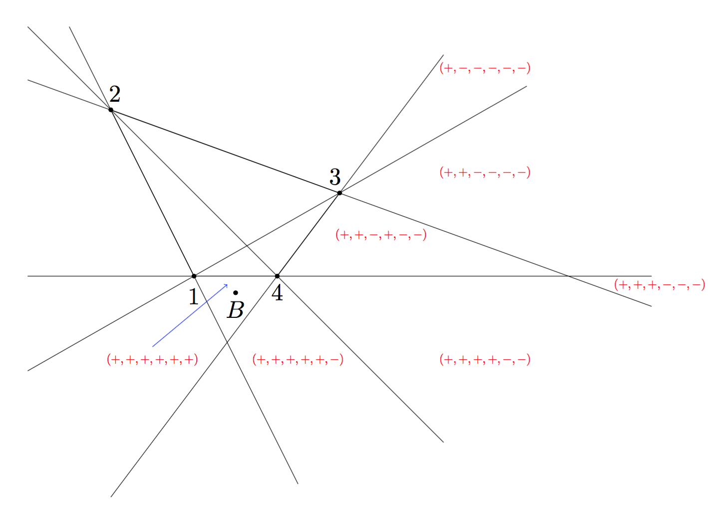
where in this picture we have labelled regions of the plane by the corresponding sign patterns of the sequence

$$\{\langle A125\rangle,\langle A135\rangle,\langle A145\rangle,\langle A235\rangle,\langle A245\rangle,\langle A345\rangle\},$$

(37)

and only configurations which give a nonzero allowed region for $B$ have been labelled. Although a priori this gives seven distinct configurations in $A$, in fact several of the configurations give identical allowed regions in $B$ and hence “glue together” naturally. If we complete this exercise for each four-point picture in Figure 9, the resulting list of configurations in $A$ and allowed regions for $B$ can be translated into the corresponding forms just as in the four point case. However, it is a less trivial exercise to compute the forms in $A$ corresponding to configurations of the $Z_{i}$. For example, one of the allowed configurations is the simple (projected) pentagon of Figure 11(a), which gives for the point $B_{\alpha}$ the triangle bounded by lines $(12)(15)(45)$. Here the codimension one boundaries in $A$ are obviously given by all deformations making three projected points collinear, so for the pentagon with ordered vertices $12345$ the poles of the form in $A$ are

$$\{\langle A123\rangle,\langle A234\rangle,\langle A345\rangle,\langle A451\rangle,\langle A512\rangle\}.$$

(38)

However, starting at five points we also find configurations such as in Figure 11(b)-(c), both of which give the region for $B_{\alpha}$ bounded by the lines (12)(15)(34), where the pole structure of the form is not as obvious. The quadrilateral configuration of Figure 11(b) has codimension one boundaries corresponding to the poles

$$\{\langle A123\rangle,\langle A134\rangle,\langle A345\rangle,\langle A145\rangle,\langle A235\rangle,\langle A125\rangle\},$$

as can easily be seen by deforming the picture in all ways which make three points collinear. However, for the triangular configuration as drawn in Figure 11(c) the relative orientation of points $Z_{3}$ and $Z_{4}$ inside the triangle is crucial in reconstructing the form, and we must indicate whether the brackets $\{\langle A134\rangle,\langle A234\rangle,\langle A345\rangle\}$ are required to have definite signs in order to satisfy the inequalities. The codimension one boundaries of this cell correspond to those collinear limits which do not first flip any brackets which have definite sign. For Figure 11(c) this gives, for example, the boundary structure corresponding to the poles

$$\{\langle A134\rangle,\langle A234\rangle,\langle A135\rangle,\langle A235\rangle,\langle A245\rangle\}.$$

The allowed regions in $B_{\alpha}$ can be classified by the pole structure of the associated form. In the four-point case we found all possible “triangles” with three poles in $B$ corresponding to the lines $(i{-}1i),(ii{+}1)$ and $(i{+}1i{+}2)$, and a priori at $n$-points one would anticipate finding triangles, quadrilaterals, etc. up to possibly $n$-gons for the allowed regions for $B_{\alpha}$. Indeed, adding a fifth point everywhere in the four-point configurations consistent with the additional five point inequalities yields both quadrilaterals and pentagons in $B_{\alpha}$. However, the corresponding sum of canonical forms for each cell does not reproduce the correct integrand on this cut at any loop order. The reason for this discrepancy is simple: in addition to the inequalities $\langle AB_{\alpha}ij\rangle>0$ we must ensure that we are only keeping configurations that are consistent with having been projected from positive data. To be more explicit, consider the following five-point configuration obtained from the procedure outlined above which is consistent with the inequalities $\langle AB_{\alpha}ij\rangle>0$ (here the point $Z_{3}$ must lie to the right of the line $(14)$ and to the left of the line $(25)$ to give the region in $B_{\alpha}$ shown)

(39)

Naïvely this configuration contributes to the cut with a quadrilateral region for $B_{\alpha}$ with poles $\langle AB12\rangle,\langle AB34\rangle,\langle AB45\rangle$ and $\langle AB15\rangle$. However, this configuration of projected $Z_{i}$ is actually inconsistent with having been projected from positive data, as a simple argument demonstrates. Namely, if we expand $Z_{5}$ in the basis $Z_{1},\ldots,Z_{4}$ we have

$$Z_{5}=\alpha_{4}Z_{4}-\alpha_{3}Z_{3}+\alpha_{2}Z_{2}-\alpha_{1}Z_{1},$$

(40)

where the positivity of the variables $\alpha_{i}>0$ follows from the positivity of the external data. Expanding the bracket $\langle A135\rangle$ using (40) and noting that $\langle A123\rangle>0$ and $\langle A134\rangle<0$ (which are conditions defining this configuration) we see this implies this bracket is negative,

$$\langle A135\rangle=\alpha_{4}\langle A134\rangle-\alpha_{3}\langle A123\rangle<0,$$

(41)

which is in contradiction to the configuration we have drawn, where $\langle A135\rangle>0$. Thus, the configuration (39) cannot be obtained by the projection of positive data.

If we cross-check the list of configurations obtained by adding a fifth point to the allowed four-point cases of Figure 9 against the positivity constraints on the external data, the surprising result is the elimination of all geometries apart from triangles in $B_{\alpha}$. The complete set of configurations can be constructed out of the following list:

		$\displaystyle(12)(23)(34)$				(42)
		$\displaystyle(12)(23)(45)$				(43)
		$\displaystyle(12)(23)(15)$				(44)
		$\displaystyle(12)(34)(45)$				(45)
		$\displaystyle(12)(34)(15)$				(46)
		$\displaystyle(12)(45)(15)$				(47)
		$\displaystyle(23)(34)(45)$				(48)
		$\displaystyle(23)(34)(15)$		$\displaystyle(\text{no sign on $\langle A245\rangle$})$		(49)
		$\displaystyle(23)(45)(15)$				(50)
		$\displaystyle(34)(45)(15)$				(51)

In these results, we have indicated the regions in $B_{\alpha}$ satisfying the one-loop inequalities by the codimension one boundaries which are lines $(ii{+}1)$ in the projection through $A$. The full set of allowed configurations is given by adding all reflections across the line $(12)$ of the above list (disregarding duplicates), which is equivalent to requiring the consideration of both cases $\langle A123\rangle\gtrless 0$. Alternatively, all possibilities can be generated by constructing, for each possible $B_{\alpha}$ region, all configurations consistent with the inequalities (with no requirements on any $\langle Aijk\rangle$ bracket); this leads to exactly the same set of allowed configurations as (42)-(51), plus reflections across $(12)$.

References

- (1) N. Arkani-Hamed, C. Langer, A.Y. Srikant and J. Trnka, Deep into the Amplituhedron: Amplitude Singularities at All Loops and Legs, Phys. Rev. Lett. 122 (2019) [arXiv:1810.08208].
- (2) N. Arkani-Hamed and J. Trnka, The Amplituhedron, JHEP 1410 (2014) [arXiv:1312.2007].
- (3) N. Arkani-Hamed, J.L. Bourjaily, F. Cachazo, A. Goncharov, A. Postnikov and J. Trnka, Scattering Amplitudes and the Positive Grassmannian.
- (4) A. Hodges, Eliminating spurious poles from gauge-theoretic amplitudes, JHEP 05 (2013) 135 [arXiv:0905.1473].
- (5) N. Arkani-Hamed, Y. Bai and T. Lam, Positive Geometries and Canonical Forms, JHEP 11 (2017) 039 [arXiv:1703.04541].
- (6) Z. Bern, E. Herrmann, S. Litsey, J. Stankowicz and J. Trnka, Logarithmic Singularities and Maximally Supersymmetric Amplitudes, JHEP 06 (2015) 202 [arXiv:1412.8584].
- (7) Z. Bern, E. Herrmann, S. Litsey, J. Stankowicz and J. Trnka, Evidence for a Nonplanar Amplituhedron, JHEP 06 (2016) 098 [arXiv:1512.08591].
- (8) Z. Bern, M. Enciso, C.H. Shen and M. Zeng, Dual Conformal Structure Beyond the Planar Limit, Phys. Rev. Lett. 121 (2018) 121603 [arXiv:1806.06509].
- (9) N. Arkani-Hamed, J.L. Bourjaily, F. Cachazo and J. Trnka, Singularity Structure of Maximally Supersymmetric Scattering Amplitudes, Phys. Rev. Lett. 113 (2014) 261603 [arXiv:1410.0354].
- (10) L. Ferro, T. Lukowski, A. Orta and M. Parisi, Yangian symmetry for the tree amplituhedron, J. Phys. A50 (2017) 294005 [arXiv:1612.04378].
- (11) L. Ferro, T. Lukowski and M. Parisi, Amplituhedron meets Jeffrey-Kirwan Residue, J. Phys. A52 (2019) 045201 [arXiv:1805.01301].
- (12) M. Enciso, Volumes of Polytopes Without Triangulations, JHEP 10 (2017) 071 [arXiv:1408.0932].
- (13) M. Enciso, Logarithms and Volumes of Polytopes, JHEP 04 (2018) 016 [arXiv:1612.07370].
- (14) S.N. Karp, L.K. Williams and Y.X. Zhang, Decompositions of amplituhedra, arXiv:1708.09525.
- (15) S.N. Karp and L.K. Williams, The amplituhedron and cyclic hyperplane arrangements, arXiv:1608.08288.
- (16) Y. Bai and S. He, The Amplituhedron from Momentum Twistor Diagrams, JHEP 02 (2015) 065 [arXiv:1408.2459].
- (17) Y. Bai, S. He and T. Lam, The Amplituhedron and the One-loop Grassmannian Measure, JHEP 01 (2016) 112 [arXiv:1510.03553].
- (18) N. Arkani-Hamed and J. Trnka, Into the Amplituhedron, JHEP 12 (2014) 182 [arXiv:1312.7878].
- (19) S. Franco, D. Galloni, A. Mariotti and J. Trnka, Anatomy of the Amplituhedron, JHEP 03 (2015) 128 [arXiv:1408.3410].
- (20) J. Rao, 4-particle Amplituhedron at 3-loop and its Mondrian Diagrammatic Implication, JHEP 06 (2018) 038 [arXiv:1712.09990].
- (21) Y. An, Y. Li, Z. Li and J. Rao, All-loop Mondrian Diagrammatics and 4-particle Amplituhedron, JHEP 06 (2018) 023 [arXiv:1712.09994].
- (22) J. Rao, 4-particle Amplituhedronics for 3-5 loops, arXiv:1806.01765.
- (23) N. Arkani-Hamed, H. Thomas and J. Trnka, Unwinding the Amplituhedron in Binary, JHEP 01 (2018) 016 [arXiv:1704.05069].
- (24) S. He and C. Zhang, Notes on Scattering Amplitudes as Differential Forms, JHEP 10 (2018) 054 [arXiv:1807.11051].
- (25) N. Arkani-Hamed, Y. Bai, S. He and G. Yan, Scattering Forms and the Positive Geometry of Kinematics, Color and the Worldsheet, JHEP 05 (2018) 096 [arXiv:1711.09102].
- (26) G. Salvatori, 1-loop Amplitudes from the Halohedron, arXiv:1806.01842.
- (27) N. Arkani-Hamed, J.L. Bourjaily, F. Cachazo and J. Trnka, Local Integrals for Planar Scattering Amplitudes, JHEP 06 (2012) 125 [arXiv:1012.6032].
- (28) J.L. Bourjaily, A. DiRe, A. Shaikh, M. Spradlin and A. Volovich, The Soft-Collinear Bootstrap: N=4 Yang-Mills Amplitudes at Six and Seven Loops, JHEP 03 (2012) 032 [arXiv:1112.6432].
- (29) J.L. Bourjaily, P. Heslop and V.V. Tran, Perturbation Theory at Eight Loops: Novel Structures and the Breakdown of Manifest Conformality in Supersymmetric Yang-Mills Theory, Phys. Rev. Lett. 116 (2016) 191602 [arXiv:1512.07912].
- (30) J.L. Bourjaily, P. Heslop and V.V. Tran, Amplitudes and Correlators to Ten Loops Using Simple, Graphical Bootstraps, JHEP 11 (2016) 125 [arXiv:1609.00007].
- (31) N. Arkani-Hamed, J.L. Bourjaily, F. Cachazo, A. Hodges and J. Trnka, A Note on Polytopes for Scattering Amplitudes, JHEP 04 (2012) 081 [arXiv:1012.6030].
- (32) N. Arkani-Hamed, A. Hodges and J. Trnka, Positive Amplitudes In The Amplituhedron, JHEP 08 (2015) 030 [arXiv:1412.8478].