Refined scattering diagrams and theta functions from asymptotic analysis of Maurer–Cartan equations

The notion of a scattering diagram was introduced by Kontsevich–Soibelman [16] and Gross–Siebert [14] in their studies of the reconstruction problem in Strominger–Yau–Zaslow mirror symmetry [25]. In this setting, scattering diagrams encode and control the combinatorial data required to consistently glue local pieces of the mirror manifold. Since their introduction, scattering diagrams have found important applications to integrable systems [17], cluster algebras [12], enumerative geometry [13] and combinatorics [24], amongst other areas. Motivated by Fukaya’s approach to the reconstruction problem [11], an asymptotic analytic perspective on scattering diagrams was developed in [6]. In this paper, we further develop this approach to give a differential geometric approach to refined and Hall algebra scattering diagrams.

The most basic form of scattering diagrams is closely related to the Lie algebra of Poisson vector fields on a torus. For many applications, it is necessary to study quantum, or refined, variants of scattering diagrams, in which the torus Lie algebra is replaced by the so-called quantum torus Lie algebra or, more generally, by an abstract monoid-graded Lie algebra satisfying a tropical condition [17, 12, 20]. For example, a number of conjectures in the theory of quantum cluster algebras were proved using scattering diagram techniques in [12]. Refined scattering diagrams were shown to be related to the refined tropical curve counting of Block–Göttsche [1] by Filippini–Stoppa [10] and Mandel [20], which also appear in study of $K3$ in [19]. These refined curve counts are also related to the refined enumeration of real plane curves by Mikhalkin [23], to higher genus Gromov–Witten invariants by Bousseau [2]. These connections could be anticipated from the central role of scattering diagrams in the reconstruction problem.

A further generalization of scattering diagrams was introduced by Bridgeland [4] under the name $\mathfrak{h}$-complex. Here $\mathfrak{h}$ is a (not-necessarily tropical) monoid-graded Lie algebra. The flexibility of allowing non-tropical Lie algebras allows one to define, for example, scattering diagrams based on the motivic Hall–Lie algebra of a three dimensional Calabi–Yau category. Bridgeland showed that each quiver with potential $(\mathsf{Q},W)$ defines a consistent $\mathfrak{h}$-complex with values in the motivic Hall–Lie algebra, the wall-crossing automorphisms of the $\mathfrak{h}$-complex encoding the motivic Donaldson–Thomas invariants of $(\mathsf{Q},W)$. Under mild assumptions, the (refined) cluster scattering diagram of $(\mathsf{Q},W)$ is then obtained by applying a Hall algebra integration map to this $\mathfrak{h}$-complex. Using these ideas, Bridgeland was able to connect scattering diagrams to the geometry of the space of stability conditions on the triangulated category associated to $(\mathsf{Q},W)$.

In [11], Fukaya suggested that much of the combinatorial behavior of instanton corrections to the $B$-side complex structure which arise near the large volume limit could be described in terms of the asymptotic limit of Maurer–Cartan elements of the Kodaira–Spencer differential graded (dg) Lie algebra. In the context of scattering diagrams, this idea was made precise and put into practice in [6], where it was shown that the asymptotic behavior of Maurer–Cartan elements of a certain dg Lie algebra admits an alternative interpretation in terms of consistent classical scattering diagrams. Moreover, the passage from an initial scattering diagram to its consistent completion, a procedure which exists due to works of Kontsevich–Soibelman [16, 17] and Gross–Siebert [14], can be understood in terms of the perturbative construction of Maurer–Cartan elements. These ideas were pursued in the setting of toric mirror symmetry to study the deformation theory of the Landau–Ginzburg mirror of a toric surface $X$ and its relation to tropical disk counting in $X$ [7].

In this paper we further develop the asymptotic approach to illustrate how refined (or more generally tropical) and Hall algebraic (or non-tropical) scattering diagrams, as well as the relevant theta functions, are controlled by asymptotic limits of Maurer–Cartan elements. To describe our results, we require some notation. Let $M$ be a lattice of rank $r$ and let $N=\Hom_{\mathbb{Z}}(M,\mathbb{Z})$. Write $M=M\otimes_{\mathbb{Z}}\real$ and $N=N\otimes_{\mathbb{Z}}\real$. Let $\sigma\subset M$ be a strictly convex cone and set $M_{\sigma}^{+}=(M\cap\sigma)\setminus\{0\}$. Let $\mathfrak{h}$ be a $M_{\sigma}^{+}$-graded Lie algebra, which for the moment we assume to be tropical.

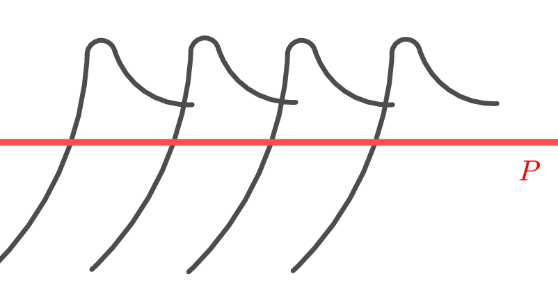
Following [6, 7], we consider differential forms on $M$ which depend on a parameter $\hslash\in\mathbb{R}_{>0}$. Let $\mathcal{W}^{0}_{*}$ be the dg algebra of such differential forms which approach a bump form along a closed tropical polyhedral subset $P\subset M_{\mathbb{R}}$ as $\hslash\rightarrow 0$. See Figure 1. The subspace $\mathcal{W}^{-1}_{*}\subset\mathcal{W}^{0}_{*}$ of differential forms which satisfy $\lim_{\hslash\rightarrow 0}\alpha=0$ is a dg ideal and

is a tropical dg Lie algebra. Our goal is to construct and interpret Maurer–Cartan elements of $\mathcal{H}^{*}$.

Our first result relates Maurer–Cartan elements of $\mathcal{H}^{*}$ to the counting of tropical disks in $M_{\mathbb{R}}$. Let $\mathscr{D}_{in}$ be an initial scattering diagram. To each wall $\mathbf{w}$ of $\mathscr{D}_{in}$, whose support is a hyperplane $P_{\mathbf{w}}$ of $M$ and whose wall-crossing factor is $\log(\Theta_{\mathbf{w}})$, we associate the term

Here $\delta_{P_{\mathbf{w}}}$ is an $\hbar$-dependent $1$-form which concentrates along $P_{\mathbf{w}}$ as $\hslash\rightarrow 0$. We take $\Pi=\sum_{\mathbf{w}\in\mathscr{D}_{in}}\Pi^{\mathbf{w}}$ as input data to solve the Maurer–Cartan equation. Our first main result, whose proof uses a modification of a method of Kuranishi [18], describes a Maurer–Cartan element $\varPhi$ constructed perturbatively from $\Pi$ using a propagator $\mathbf{H}$ (see Section 3.1.1).

In Section 3.2 we associate to the Maurer–Cartan element $\varPhi$ a scattering diagram $\mathscr{D}(\varPhi)$. The walls of $\mathscr{D}(\varPhi)$ are labeled by the maximal cells $\sigma$ of the polyhedral decompositions $\mathcal{P}_{L}$ and have wall-crossing automorphisms $\exp(\frac{c_{L,\sigma}}{|\text{{Aut}}(L)|}g_{L})$. The diagram $\mathscr{D}(\varPhi)$ extends $\mathscr{D}_{in}$ and is in fact a consistent scattering diagram; see Proposition 3.14. In this way, we obtain an enumerative interpretation of the consistent completion of $\mathscr{D}_{in}$.

Next, we turn to theta functions. Let $\mathcal{C}$ be a cone satisfying $\sigma\subset\mathcal{C}\subset M$ with associated monoid $P=\mathcal{C}\cap M$ and let $A$ be a $P$-graded algebra with a graded $\mathfrak{h}$-action. The dg Lie algebra $\mathcal{H}^{*}$ acts naturally on the dg algebra

Given a Maurer–Cartan element $\varPhi\in\mathcal{H}^{*}$, it is natural to study the space of flat sections $\text{Ker}(d_{\varPhi})$ of the deformed differential $d_{\varPhi}=d+[\varPhi,\cdot]$. The algebra structure on $\mathcal{A}^{*}$ induces an algebra structure on $\Ker(\varPhi)$. The following result describes the wall-crossing behavior of the $\hslash\rightarrow 0$ limit of flat sections.

To connect with theta functions, we work in the square zero extension dg Lie algebra $\mathcal{H}^{*}\oplus\mathcal{A}^{*}[-1]$ where, for each $m\in P$, we perturbatively solve the Maurer–Cartan equation with input $\Pi+z^{m}$. The resulting Maurer–Cartan element is of the form $\varPhi+\theta_{m}$, with $\varPhi$ as above and $\theta_{m}\in\Ker(d_{\varPhi})$. On the other hand, associated to $m\in P$ is the (standard) theta function

defined in terms of broken lines ending at $(m,Q)$, that is, piecewise linear maps $\gamma:(-\infty,0]\rightarrow M$ which bend only at the walls of $\mathscr{D}(\varPhi)$. Each broken line $\gamma$ has an associated weight $a_{\gamma}\in A$.

Finally, in Section 3.4 we study the above constructions in the setting of non-tropical Lie algebras. One advantage of the differential geometric approach of this paper is that it is applicable to non-generic cases without perturbing $\mathscr{D}_{in}$. With a mild commutativity condition on the wall-crossing automorphisms of the walls of $\mathscr{D}_{in}$ which, for example, is satisfied in the Hall algebra setting, we obtain new results in the non-tropical case, where perturbation of $\mathscr{D}_{in}$ is not possible. Theorem 3.27 generalizes to the non-tropical setting the construction of a Maurer–Cartan element $\varPhi$ from an initial scattering diagram $\mathscr{D}_{in}$ and associates to $\varPhi$ a consistent completion of $\mathscr{D}_{in}$. We also prove that the completed scattering diagram is equivalent to that constructed algebraically by Bridgeland [4]. Moreover, we construct, for each $n\in N_{\sigma}^{+}$, a theta function $\theta_{n}\in\Ker(d_{\varPhi})$ as a perturbative Maurer–Cartan element and prove that it agrees with Bridgeland’s Hall algebra theta function [4].

In Section 3.4.5 we restrict attention to the case in which the Lie algebra is the motivic Hall–Lie algebra of an acyclic quiver. In this case, there is a canonical choice for the propagator $\mathbf{H}$, leading to a combinatorial formula for $\varPhi$ and $\theta_{n}$ in terms of tropical disks.

Here $\mathtt{L}\mathtt{T}_{k}$ and $\mathtt{M}\mathtt{T}_{k}$ are the sets of labeled, respectively marked, $k$-trees and $g_{L}$, $a_{J}$ are Hall algebraic Block–Göttsche-type multiplicities. The formula for $\theta_{n}$ can be regarded as a replacement for a description of $\vartheta_{n,Q}$ in terms of Hall algebra broken lines. Indeed, it was recently shown by Cheung and Mandel [9] that, contrary to Bridgeland’s theta functions, Hall algebra theta functions which are defined in terms of Hall algebra broken lines do not, in general, satisfy the wall-crossing formula.

The authors would like to thank Kwokwai Chan, Man-Wai Cheung and Travis Mandel for many useful discussions and suggestions. Naichung Conan Leung was supported in part by a grant from the Research Grants Council of the Hong Kong Council of the Hong Kong Special Administrative Region, China (Project No. CUHK 14302215 and 14303516).

Following [12, 20], we recall the definition of scattering diagrams. Compared to [20], the roles of $M$ and $N$ are reversed.

We follow [20] to define broken lines. Fix a consistent scattering diagram $\mathscr{D}$ over $R$.

In the notation of Definition 1.7, we will write $a_{\gamma}$ for $a_{l}$.

In the present setting, well-definedness of theta functions was proved in [20]. Observe that $\vartheta_{\mathsf{m},Q}\in z^{\varphi(\mathsf{m})}+\hat{A}_{\varphi(\mathsf{m})+M_{\sigma}^{+}},$ where $\hat{A}_{\varphi(\mathsf{m})+M_{\sigma}^{+}}$ is the completion of $A_{\varphi(\mathsf{m})+M_{\sigma}^{+}}\otimes_{\mathbb{C}}R$.

We recall some definitions from [20], modified so as to incorporate the work of [6]. Fix a scattering diagram $\mathscr{D}_{in}=\{\mathbf{w}_{i}=(m_{i},n_{i},P_{i},\Theta_{i})\}_{i\in I}$ and let $g_{i}=\log(\Theta_{i})$. Write

For each $l\geq 0$, define commutative rings $R=\mathbb{C}[\{t_{i}\mid i\in I\}]$ and $R_{l}=\mathbb{C}[\{t_{i}\mid i\in I\}]/\langle t_{i}^{l+1}\ |\ i\in I\rangle$, as in [13, 20]. There is a ring homomorphism

We follow [6, 10, 13, 22] and introduce tropical disks in $\mathscr{D}_{in}$ or $\tilde{\mathscr{D}}_{in,l}$.

Two $k$-trees are isomorphic if there exist bijections between their sets of vertices and edges which preserve the respective decompositions and boundary maps. Set $T^{[0]}_{\infty}=T_{in}^{[0]}\sqcup\{v_{out}\}$ and $T^{[1]}=\bar{T}^{[1]}\setminus\partial_{in}^{-1}(T^{[0]}_{in})$. The edge $e_{out}:=\partial_{out}^{-1}(v_{out})$ is called the outgoing edge. The root vertex $v_{r}$ is the unique vertex satisfying $e_{out}=\partial^{-1}_{in}(v_{r})$.

Two labeled $k$-trees are isomorphic if they are isomorphic as $k$-trees by a label preserving isomorphism, and similarly for marked and weighted cases. The set of isomorphism classes of labeled, marked and weighted $k$-trees will be denoted by $\mathtt{L}\mathtt{T}_{k}$, $\mathtt{M}\mathtt{T}_{k}$ and $\mathtt{W}\mathtt{T}_{k}$, respectively.

Let $L$ be a labeled $k$-tree. Inductively define a labeling of all edges of $L$ by requiring that for a vertex $v\in L^{[0]}$ with incoming edges $e_{1},e_{2}$ (so that $\partial_{out}^{-1}(v)=\{e_{1},e_{2}\}$) and outgoing edge $e_{3}$, the equality $m_{e_{3}}=m_{e_{1}}+m_{e_{2}}$ holds. A similar procedure applies to marked and weighted $k$-trees, where in the latter case we also require $u^{\vec{J}_{e_{3}}}=u^{\vec{J}_{e_{1}}}u^{\vec{J}_{e_{2}}}$. Write $m_{L/\penalty J/\penalty\Gamma}=m_{e_{out}}$ and $u^{\vec{J}_{\Gamma}}=u^{\vec{J}_{e_{out}}}$.

Labeled ribbon $k$-trees are isomorphic if they are isomorphic as $k$-trees by an isomorphism which preserves the ribbon structure and labels. The set of isomorphism classes of labeled ribbon $k$-trees will be denoted by $\mathtt{L}\mathtt{R}_{k}$. Similarly, $\mathtt{M}\mathtt{R}_{k}$ and $\mathtt{W}\mathtt{R}_{k}$ are the sets of isomorphism classes of marked and weighted ribbon $k$-trees, respectively. Note that the topological realization of a labeled (or marked, weighted) ribbon $k$-tree $\mathcal{L}$ admits a canonical embedding into the unit disc $D$ so that $\mathcal{L}^{[0]}_{\infty}\subset\partial D$.

Write $(n_{L},g_{L})$ or $(n_{\Gamma},g_{\Gamma})$ for the pair associated to $e_{out}$. Note that if $v\in\Gamma^{[0]}$ has incoming edges $e_{1},e_{2}$ and outgoing edge $e_{3}$ and $m_{e_{1}},m_{e_{2}}\in M$ are linearly dependent, then $n_{e_{3}}=0$ and hence $g_{\Gamma}=0$, as follows from the vanishing $\mathfrak{h}_{m,0}=\{0\}$.

References

• [1] F. Block and L. Göttsche. Refined curve counting with tropical geometry. Compos. Math., 152(1):115–151, 2016.
• [2] P. Bousseau. Tropical refined curve counting from higher genera and lambda classes. Invent. Math., 215(1):1–79, 2019.
• [3] T. Bridgeland. An introduction to motivic Hall algebras. Adv. Math., 229(1):102–138, 2012.
• [4] T. Bridgeland. Scattering diagrams, Hall algebras and stability conditions. Algebr. Geom., 4(5):523–561, 2017.
• [5] M. Carl, M. Pumperla, and B. Siebert. A tropical view on Landau-Ginzburg models. Preprint, 2010.
• [6] K.-W. Chan, N. C. Leung, and Z. N. Ma. Scattering diagram from asymptotic analysis on Maurer-Cartan equation. arXiv:1807.08145, 2018.
• [7] K.-W. Chan and Z. N. Ma. Tropical disk counting from asymptotic analysis on Maurer-Cartan equation. arXiv:1807.08159, 2018.
• [8] M.-W. Cheung. Tropical techniques in cluster theory and enumerative geometry. PhD thesis, UC San Diego, 2016.
• [9] M.-W. Cheung and T. Mandel. Donaldson-Thomas invariants from tropical disks. arXiv:1902.05393, 2019.
• [10] S. Filippini and J. Stoppa. Block-Göttsche invariants from wall-crossing. Compos. Math., 151(8):1543–1567, 2015.
• [11] K. Fukaya. Multivalued Morse theory, asymptotic analysis and mirror symmetry. In Graphs and patterns in mathematics and theoretical physics, volume 73 of Proc. Sympos. Pure Math., pages 205–278. Amer. Math. Soc., Providence, RI, 2005.
• [12] M. Gross, P. Hacking, S. Keel, and M. Kontsevich. Canonical bases for cluster algebras. J. Amer. Math. Soc., 31(2):497–608, 2018.
• [13] M. Gross, R. Pandharipande, and B. Siebert. The tropical vertex. Duke Math. J., 153(2):297–362, 2010.
• [14] M. Gross and B. Siebert. From real affine geometry to complex geometry. Ann. of Math. (2), 174(3):1301–1428, 2011.
• [15] D. Joyce. Configurations in abelian categories. II. Ringel-Hall algebras. Adv. Math., 210(2):635–706, 2007.
• [16] M. Kontsevich and Y. Soibelman. Affine structures and non-Archimedean analytic spaces. In The unity of mathematics, volume 244 of Progr. Math., pages 321–385. Birkhäuser Boston, Boston, MA, 2006.
• [17] M. Kontsevich and Y. Soibelman. Wall-crossing structures in Donaldson-Thomas invariants, integrable systems and mirror symmetry. In Homological mirror symmetry and tropical geometry, volume 15 of Lect. Notes Unione Mat. Ital., pages 197–308. Springer, Cham, 2014.
• [18] M. Kuranishi. New proof for the existence of locally complete families of complex structures. In Proc. Conf. Complex Analysis (Minneapolis, 1964), pages 142–154. Springer, Berlin, 1965.
• [19] Y.-S. Lin. On the Refined of Open Gromov-Witten invariants on K3 Surfaces. ICCM Proceedings 2016.
• [20] T. Mandel. Scattering diagrams, theta functions and refined tropical curve counts. arXiv:1503.06183, 2015.
• [21] M. Manetti. Differential graded Lie algebras and formal deformation theory. In Algebraic geometry—Seattle 2005. Part 2, volume 80 of Proc. Sympos. Pure Math., pages 785–810. Amer. Math. Soc., Providence, RI, 2009.
• [22] G. Mikhalkin. Enumerative tropical algebraic geometry in ℝ2\mathbb{R}^{2}. J. Amer. Math. Soc., 18(2):313–377, 2005.
• [23] G. Mikhalkin. Quantum indices and refined enumeration of real plane curves. Acta Mathematica, 219(1):135–180, 2017.
• [24] N. Reading. Scattering fans. arXiv:1712.06968, 2017.
• [25] A. Strominger, S.-T. Yau, and E. Zaslow. Mirror symmetry is TT-duality. Nuclear Phys. B, 479(1-2):243–259, 1996.