Detection of Hermitian connections in wave equations with cubic non-linearity

Let $(M,g)$ be a Lorentzian manifold of dimension $1+3$ and consider a compact Lie group $G$ with Lie algebra $\mathfrak{g}$. We choose a positive definite inner product on $\mathfrak{g}$ invariant under the adjoint action. To simplify the exposition we discuss the case of the trivial bundle $M\times\mathfrak{g}$ over $M$. The Yang-Mills-Higgs equations are PDEs on a pair $(A,\Phi)$, where

Since the bundle $M\times\mathfrak{g}$ is trivial, $A$ is a connection, and it is called the Yang-Mills potential; $\Phi$ is the Higgs field. The Yang-Mills-Higgs equations are

where $F_{A}:=dA+A\wedge A$ is the curvature of $A$, $D_{A}\Phi:=d\Phi+[A,\Phi]$ is the associated covariant derivative, and $V^{\prime}$ is the derivative of a smooth function $V:[0,\infty)\to\mathbb{R}$. The adoint $D_{A}^{*}$ is taken with respect to $g$ and hence $\Box_{A}:=D_{A}^{*}D_{A}$ is the wave operator associated with $g$ and $A$.

An extensively studied case is the Yang-Mills-Higgs equations with the Mexican hat type potential,

where $\kappa,b\in\mathbb{R}$, see e.g. [8, Eq. (10.5)] where the Lagrangian formulation of the problem is used. We will consider the potential (3) with $\kappa\neq 0$, and to simplify the notations, with $b=0$. The case $b\neq 0$ is not substantially different. Our choice can be viewed as the simplest potential introducing a non-linearity. We refer also to [36] where Yang-Mills-Higgs equations, with the potential (3), are discussed in a purely mathematical context, $(M,g)$ being a Riemannian manifold there.

As it is well known, equations (1)–(2) are invariant under the group of gauge transformations which in this case coincides with the set of maps $\mathbf{u}\in C^{\infty}(M;G)$ and the action on pairs is

When $\Phi=0$ we obtain the pure Yang-Mills equation $D_{A}^{*}F_{A}=0$.

Dealing with the equations (1)–(2) from the outset might be too ambitious, so here we propose a simplified model. We shall suppose that we have a trivial bundle $E=M\times\mathbb{C}^{n}$ and a Hermitian connection $A$ on $E$ giving rise to a covariant derivative $d+A$. In this case, the gauge group is $U(n)$. We take $V$ to be the Mexican hat type potential (3) with $b=0$, discard equation (1) completely and focus on the analogue of equation (2), with $M\times\mathfrak{g}$ replaced by $E$. That is, we consider the equation

where $\phi$ is a section of $E$, $\Box_{A}=(d+A)^{*}(d+A)$ and $|\phi|$ is the norm with respect to the standard Hermitian inner product of $\mathbb{C}^{n}$. We shall further simplify matters by assuming that $M$ is $\mathbb{R}^{1+3}$ and that $g$ is the Minkowski metric.

Let us consider Cartesian coordinates $(t=x^{0},x^{1},x^{2},x^{3})$ on $\mathbb{R}^{1+3}$. Let $\epsilon_{0}>0$ and define $B(\epsilon_{0})=\{y\in\mathbb{R}^{3}:|y|<\epsilon_{0}\}$ and

We will formulate a source-to-solution map, associated to (4), that corresponds physically to measurements gathered in $\mho$. We can think that the measurements are performed by an observer travelling along the path

In what follows, we consider only finite time intervals, and write $\mathcal{M}=(-1,2)\times\mathbb{R}^{3}$. and let $\mathcal{C}$ be a small neighbourhood of the zero section in $C_{0}^{4}(\mho;E)$. Then the source-to-solution map

is well-defined, where $\phi$ is the solution of

We discuss the existence of $L_{A}$ in more detail in Section 2 below.

The goal of the observer is to determine the Yang-Mills potential $A$ up to the natural obstructions, given the source-to-solution map $L_{A}$. The causal structure of $(M,g)$ encodes the finite speed of propagation for the wave equation (4). Given $x,y\in M$ we say that $x\leq y$ if $x=y$ or $x$ can be joined to $y$ by a future pointing causal curve, and denote the causal future of $x\in M$ by $\mathscr{J}^{+}(x)=\{y\in M:\;x\leq y\}$. The causal future $\mathscr{J}^{+}(x)$ is the largest set that waves generated at $x$ can reach. The causal past of a point $z\in M$ is denoted by $\mathscr{J}^{-}(z)=\{y\in M:\;y\leq z\}$. If waves generated at $x$ are recorded at $z$, the finite speed of propagation dictates that no information on the potential $A$ outside the causal diamond $\mathscr{J}^{+}(x)\cap\mathscr{J}^{-}(z)$ is obtained.

The model problem is to determine $A$ given $L_{A}$ in the largest domain possible, that is, in

up to the natural gauge,

where $\mathbf{u}\in C^{\infty}(\mathbb{D};U(n))$ and $\mathbf{u}|_{\mho}=\id$. The sets $\mho$ and $\mathbb{D}$ are visualized in Figure 2.

Observe that if we have two connections $A$ and $B$ on $M$ such that there exists a smooth map $\mathbf{u}:\mathcal{M}\to U(n)$ with the property that $B=\mathbf{u}^{-1}d\mathbf{u}+\mathbf{u}^{-1}A\mathbf{u}$ and $\mathbf{u}|_{\mho}=\text{id}$, then $\Box_{B}=\mathbf{u}^{-1}\Box_{A}\mathbf{u}$ and $|\mathbf{u}\phi|=|\phi|$. Moreover, as $f$ has compact support in $\mho$ it holds that $\mathbf{u}f=f$. Therefore $\phi$ solves (8) for $B$ if and only if $\mathbf{u}\phi$ solves (8) for $A$, and it follows that $L_{A}=L_{B}$. This shows that the gauge (10) is indeed natural.

Our main theorem asserts that the model problem has a unique solution, or in more physical terms, the measurements performed on $\mho$, as encoded by $L_{A}$, determine the gauge equivalence class of the Yang-Mills potential $A$, in the largest possible causal diamond $\mathbb{D}$. As $\mathbb{D}$ is strictly larger than $\mho$, we can view the determination of the equivalence class of $A$ as a form of remote sensing. We emphasize that the gauge equivalence classes of Yang-Mills potentials, not the potentials themselves, correspond to physically distinct configurations.

It is straightforward to see that $L_{A}=L_{B}$ implies $A=B$ on $\mho$. The non-trivial content of the theorem is the gauge equivalence away from $\mho$. To see that $A$ and $B$ coincide on $\mho$, we fix $y\in\mho$ and choose $\phi\in C_{0}^{\infty}(\mho;E)$ such that $\phi(y)=0$. Then for small $\epsilon>0$ it holds that $f:=\epsilon(\Box_{A}\phi+\kappa|\phi|^{2}\phi)\in\mathcal{C}$. Since $L_{A}=L_{B}$ we see that at $y$:

cf. (14) below, and since $d\phi$ at $y$ is arbitrary, there holds $A=B$ at $y$.

The previous results on inverse problems for non-linear wave equations, such as [20, 23, 28], are based on analysis of four singular, interacting waves. A new feature in the present paper is that we consider interactions of three waves only. This leads to a more economic proof, and is particularly well suited for the cubic non-linearity in (8). A more detailed comparison of interaction three versus four waves is given in the beginning of Section 3.1.

Let us briefly explain what we mean by the interactions of three waves. The idea is to choose a source of the form $f=\epsilon_{1}f_{1}+\epsilon_{2}f_{2}+\epsilon_{3}f_{3}$ where $\epsilon_{j}>0$ are small and $f_{j}$ are conormal distributions. Then the cross-derivative $\partial_{\epsilon_{1}}\partial_{\epsilon_{2}}\partial_{\epsilon_{3}}\phi|_{\epsilon=0}$ satisfies a linear wave equation with a right-hand side that corresponds to a certain product of $\partial_{\epsilon_{j}}\phi|_{\epsilon=0}$, $j=1,2,3$. Here $\epsilon=(\epsilon_{1},\epsilon_{2},\epsilon_{3})$. As also the functions $\partial_{\epsilon_{j}}\phi|_{\epsilon=0}$ satisfy the linear wave equation, we can view the cross-derivative as a result of their interaction.

The wave front set of the above cross-derivative was studied in the case of the $1+2$-dimensional Minkowski space by Rauch and Reed [32], see also [6, 30] for later results of similar nature. What is new in the present paper, is that, contrary to [32] and the previous results on inverse problems for non-linear wave equations, e.g. [20, 23, 28], we employ more precise information on the singular structure of the cross derivative than just its wave front set. Namely, in a suitable microlocal sense, the cross-derivative has a principal symbol, and the proof of Theorem 1 uses information contained in the principal symbol in order to recover a novel broken non-abelian light ray transform of the connection $A$ along lightlike geodesics. The proof of Theorem 1 is completed by solving the subsidiary geometric inverse problem of inverting this transform in the Minkowski space, see Proposition 2 below, a result which has independent interest.

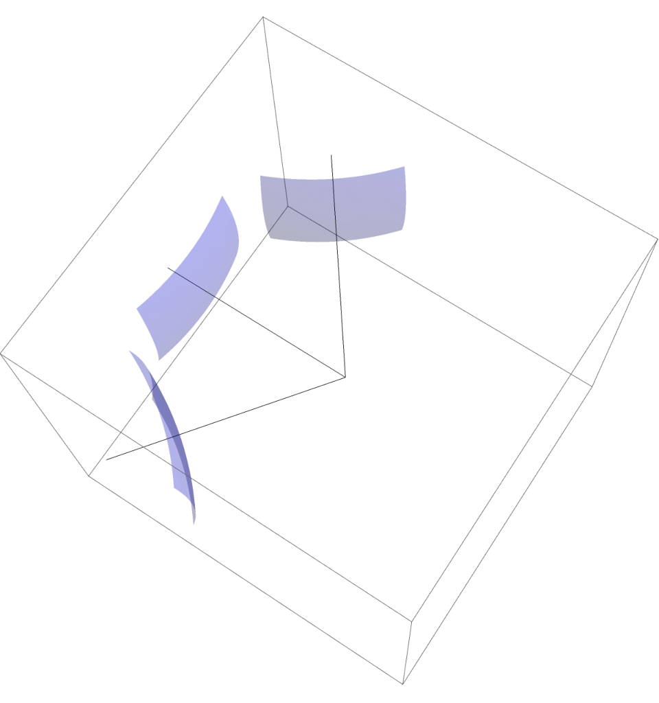
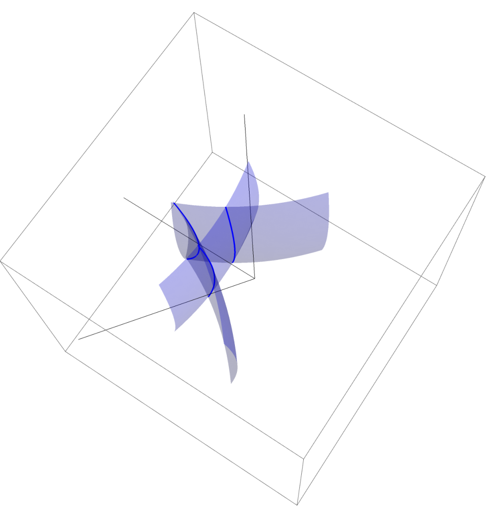
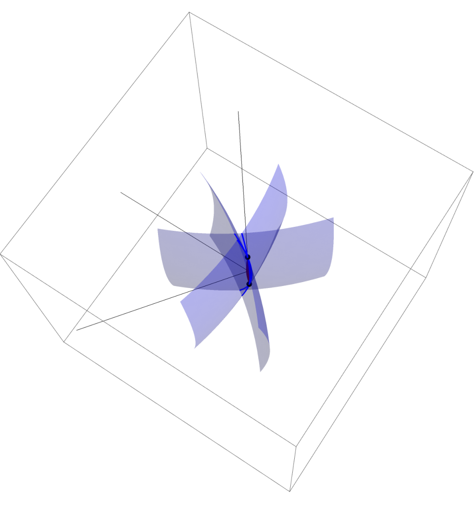
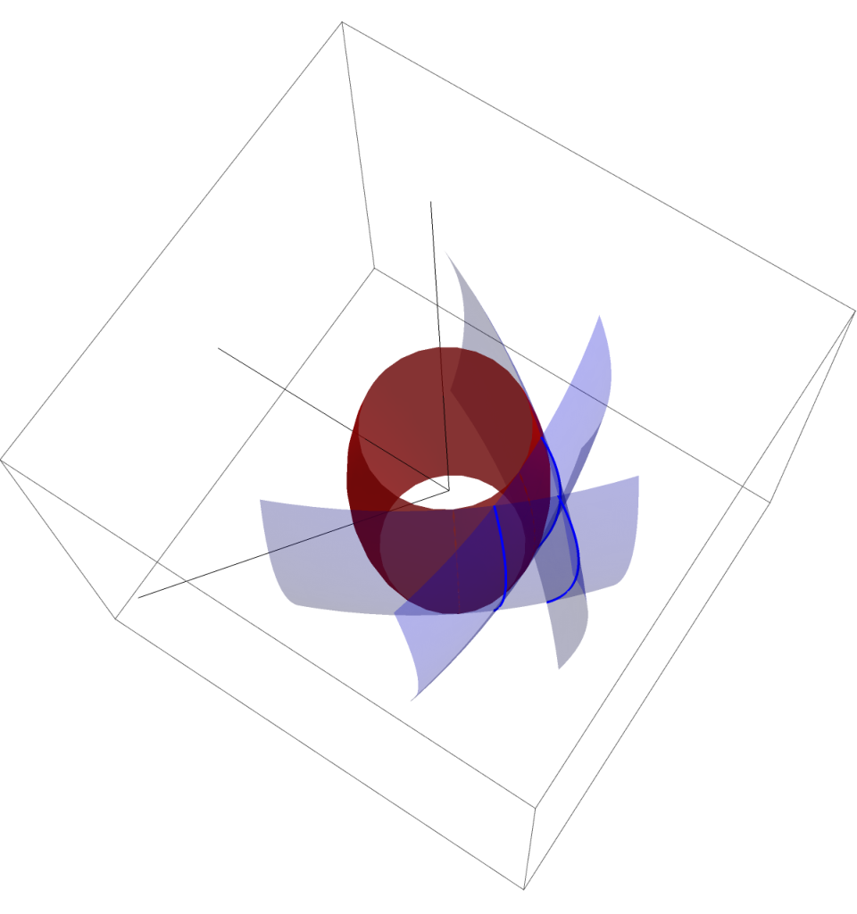
In more physical terms, we can say that the interaction of the three waves $\partial_{\epsilon_{j}}\phi|_{\epsilon=0}$, $j=1,2,3$, produce an artificial source, that can be viewed either as two moving point sources or as a filament in spacetime, and that emits a wave encoded by the cross-derivative $\partial_{\epsilon_{1}}\partial_{\epsilon_{2}}\partial_{\epsilon_{3}}\phi|_{\epsilon=0}$. We show that, when the sources $f_{j}$, $j=1,2,3$, are chosen carefully, the singular wave front emitted by the artificial source returns to $\mho$. This wave front is visualized in Figure 1. Stretching the physical analogy further, we can say the leading amplitude of this singular wave front is the information used in the proof.

Paradoxically, Theorem 1 is open for the linear case, $\kappa=0$, but a positive solution is known if $A$ and $B$ are supposed to be time-independent [24]. In the time-dependent case there are results [34] available only in the abelian case of a line bundle, $n=1$, and it is an open problem if recovery of $A$ in the optimal causal diamond $\mathbb{D}$ is possible in this case. Let us also mention that the linear, abelian, time-independent case has been studied extensively, see e.g. [2, 3, 17], but these results do not carry over to the time-dependent case. The reason for this is that they (and also above mentioned [24]) are based on Tataru’s unique continuation principle [35], that again is known to fail for equations with time-dependent coefficients [1].

We emphasize once more that the focus of the current paper is on the recovery of the lower order terms in a non-linear wave equation. This makes definite progress towards Open Problem 5 in [25], and is different from the previous results where only the determination of the leading order terms is considered. See for instance [23, 28] where the determination of the metric tensor (or its conformal class) is studied for scalar-valued non-linear equations, or [20, 27] where the determination of the metric tensor is studied for the Einstein equations coupled with different matter field equations. The difference between recovery of leading and lower order terms is reflected in the key novelty of our approach, namely, in the study of principal symbols instead of wave front sets.

Such difference is apparent also in the existing theory of inverse problems for linear wave equations. The case of a linear wave equation with time independent coefficients, and with sources and observations in disjoint sets, illustrates this. In this case the theory is still under active development, and the best results available are very different for leading and lower order terms: the recovery of the metric [26] is based on distance functions, whereas the recovery of the lower-order terms [19] is based on focussing of waves. The latter also requires additional convexity assumptions, that are not present in the former case.

One outcome of the current paper is the following emergent principle for dealing with inverse problems for waves with polynomial non-linearities using an approach similar to ours. Assume for simplicity that we are in the line bundle case (i.e. $n=1$) and consider an equation of the form

where $\kappa\neq 0$. Then to recover $A$ (up to gauge) from a source-to-solution map it is necessary to consider the $J$-fold linearization of (11), where

The necessity is discussed further in Remarks 2 and 4 below. We conjecture that (12) is also a sufficient condition, but the present paper establishes this only in the case $N=3$.

This paper is organized as follows. Section 2 contains preliminaries mostly having to do with the direct problem (8). Section 3 contains the microlocal analysis for the interaction of three waves and shows that we can recover the broken non-abelian light ray transform along lightlike geodesics from the knowledge of $L_{A}$. Section 4 solves the geometric inverse problem of determining $A$ up to gauge from the broken non-abelian light ray transform and completes the proof of Theorem 1. Appendix A recalls the theory of conormal and Intersecting Pair of Lagrangian (IPL) distributions; Appendix B contains certain technical details concerning symplectic transformations to a model pair of intersecting Lagrangians, and Maslov bundles; and Appendix C gives full description of the wave front set of the cross-derivative $\partial_{\epsilon_{1}}\partial_{\epsilon_{2}}\partial_{\epsilon_{3}}\phi|_{\epsilon=0}$, that is, the red surface in Figure 1.

ML was supported by Academy of Finland grants 320113 and 312119. LO was supported by EPSRC grants EP/P01593X/1 and EP/R002207/1 and XC and GPP were supported by EPSRC grant EP/R001898/1. GPP thanks the University of Washington for hospitality while this work was in progress and the Leverhulme trust for financial support.

We write occasionally $\nabla=d+A$ for the covariant derivative associated to the connection $A$, and view it as a map

Writing $g=g_{ij}dx^{i}dx^{j}$ in coordinates, we denote by $|g|$ and $g^{ij}$ the determinant and inverse of $g_{ij}$, respectively. Moreover, $A=A_{j}dx^{j}$ is a $1$-form, and each $A_{j}$ is a skew-Hermitian matrix. Let us now write the wave operator $\Box_{A}=\nabla^{*}\nabla$ in coordinates. Consider compactly supported sections $\phi$ and $\psi=\psi_{j}dx^{j}$ of $E$ and $T^{\ast}M\otimes E$, respectively. Then

where $\langle\cdot,\cdot\rangle_{E}$ is the inner product on $E$, and $dV_{g}$ denotes the volume form on $(M,g)$. Integrating by parts and using the fact that $A$ is skew-Hermitian, we have

Consequently, $\Box_{A}\phi$ takes the form

Let $T>0$ and let us consider the following nonlinear Cauchy problem

where $H:(\mathbb{R}\times M_{0})\times E\to E$ is a smooth map operating section-wise such that $H(t,x,0)=0$, and $f$ is a section of $E$. We will now give sufficient conditions on $f$ in order for (15) to have a unique solution.

As the leading term of $\Box_{A}$ is simply the canonical wave operator on $(M,g)$, acting on each component of $\phi$, we can use the standard results for quasilinear hyperbolic equations to show existence and uniqueness of solutions to this Cauchy problem. See, for example, Theorem 6 of [18] and its proof (with the notations explained in detail in Appendix C in [21]) or Theorems I-III and the proof of Lemma 2.7 in [15]. By these results, we have that for an integer $r>m/2+2$ and any compact set $\mathcal{K}\subset(0,T)\times M_{0}$, there is $\epsilon_{0}>0$ such that for any $f\in C^{r}_{0}(\mathcal{K})$ satisfying $\|f\|_{C^{r}(\mathcal{K})}<\epsilon_{0}$, the initial value problem (15) has a unique solution. Recall that $m$ is the dimension of the underlying space $M_{0}$. In particular, in the case of the Minkowski space $\mathbb{R}^{1+3}$, we may take $r=4$, and see that source-to-solution map $L_{A}$ is well-defined by (7).

For a conic Lagrangian submanifold $\Lambda_{0}\subset T^{*}M\setminus 0$ and a vector bundle $\mathbb{E}$ over $M$, we denote by $I^{p}(M;\Lambda_{0};\mathbb{E})$ the space of Lagrangian distributions of order $p\in\mathbb{R}$ associated to $\Lambda_{0}$, and taking values in $\mathbb{E}$. If $\Lambda_{1}\subset T^{*}M\setminus 0$ is another conic Lagrangian submanifold intersecting $\Lambda_{0}$ cleanly, we denote by $I^{p}(M;\Lambda_{0},\Lambda_{1};\mathbb{E})$ the space of Intersecting Pair of Lagrangian (IPL) distributions of order $p\in\mathbb{R}$ associated to $(\Lambda_{0},\Lambda_{1})$, and taking values in $\mathbb{E}$.

We use occasionally the notation $\left\langle\cdot,\cdot\right\rangle$ for the duality pairing between covectors and vectors, and

If $\Lambda_{0}$ coincides with the conormal bundle

of a submanifold $K\subset M$ in the sense that $\Lambda_{0}=N^{*}K\setminus 0$, then the distributions in $I(M;\Lambda_{0};\mathbb{E})$ are called conormal distributions. Although removing the zero section from $N^{*}K$, when considering it as a conic Lagrangian manifold, is somewhat awkward notationally, it is natural to consider $N^{*}K$ as a submanifold of $T^{*}M$, since then the fibres $N_{x}^{*}K\subset T_{x}^{*}M$, $x\in K$, are linear subspaces. We recall the basic properties of conormal and IPL distributions in Appendix A below.

The wave front set of a distribution $u\in\mathcal{D}^{\prime}(M)$ is denoted by $\WF(u)$, see [11, Def. 2.5.2]. It is a subset of $T^{*}M\setminus 0$, and its projection on $M$ is called the singular support $\singsupp(u)$ of $u$. The wave front set $\WF(u)$ is conical and closed in $T^{*}M\setminus 0$, and it is occasionally convenient to use the notation

for the conical closure of a set $\mathscr{B}\subset T^{*}M\setminus 0$. For $u\in I(M;\Lambda_{0};\mathbb{E})$ it holds that $\WF(u)\subset\Lambda_{0}$.

If $\mathscr{K}$ is the Schwartz kernel of a pseudodifferential operator $\chi$ on $M$, then the projection of $\WF(\mathscr{K})\subset(T^{*}M\setminus 0)^{2}$ on the first factor $T^{*}M\setminus 0$ is called the essential support of $\chi$. (As $\WF(\mathscr{K})$ is contained in the conormal bundle of the diagonal $\{(x,y)\in M^{2}:x=y\}$, the choice between the first and second factor makes no difference.) Following [11, p. 124] we write $\WF(\chi)$ for this set.

We denote by $\Omega^{1/2}$ the half-density bundle over $M$. When $\Lambda_{0}$ and $\Lambda_{1}\setminus\Lambda_{0}$ coincide with conormal bundles, and $\mathbb{E}=E\otimes\Omega^{1/2}$, there is a coordinate invariant way to define the principal symbol $\sigma[u]$ of $u\in I(M;\Lambda_{0};\mathbb{E})$, respectively $u\in I(M;\Lambda_{0},\Lambda_{1};\mathbb{E})$, as an equivalence class of sections of $E\otimes\Omega^{1/2}$ over $\Lambda_{0}$, respectively $\Lambda_{1}\setminus\Lambda_{0}$. We will not emphasize the difference between the equivalence class $\sigma[u]$ and a representative of it, and we will also use the same notation for the half-density bundles over $M$ and $\Lambda_{j}$, $j=0,1$. Let us remark that there is typically no natural way to relate these bundles. For example, while it is natural to use $|g|^{1/4}$ to trivialize $\Omega^{1/2}$ over $M$, the Lorentzian metric $g$ on $M$ typically does not induce a natural trivialization of $\Omega^{1/2}$ over $\Lambda_{j}$.

For IPL distributions in $I(M;\Lambda_{0},\Lambda_{1};\mathbb{E})$, there is also a refined notion of principal symbol, with components on both $\Lambda_{0}$ and $\Lambda_{1}$. We will use the refined principal symbol only in Appendix A. The notation $\sigma[\chi]$ is used also for the principal symbol of a pseudodifferential operator $\chi$ on $M$. In this case, $\sigma[\chi]$ is represented by a section of $T^{*}M\setminus 0$.

It is convenient to rescale (8), and consider the following non-linear wave operator

where $|\cdot|=|\cdot|_{E}$ is the norm with respect to the inner product $\langle\cdot,\cdot\rangle=\langle\cdot,\cdot\rangle_{E}$. In order to make use of the microlocal machinery developed in [9], we conjugate the operator $Q_{0}$ with the half density $|g|^{1/4}$ and consider the operator $Q(u):=|g|^{1/4}Q_{0}(|g|^{-1/4}u)$ acting on the sections of $E\otimes\Omega^{1/2}$. Writing $Pu=|g|^{1/4}\Box_{A}(|g|^{-1/4}u)/2$, the operator $Q$ reads

For the sake of convenience, we will slightly abuse the notation, and write

for products of half-densities as functions. Then $Q(u)=Pu+\kappa|u|^{2}u/2$.

Writing $\imath=\sqrt{-1}$, the full symbol of the operator $P$ reads

and we see that $P$ has the following principal symbol $\sigma[P]$ and subprincipal symbol $\sigma_{sub}[P]$, in the sense of Duistermaat and Hörmander [9, p.189 (5.2.8)],

We write also $\sigma[P]=\left\langle\xi,\xi\right\rangle_{g}/2$ where $\left\langle\xi,\xi\right\rangle_{g}$ denotes the inner product with respect to $g$. Let us remark that the subprincipal symbol transforming as a connection is discussed in [16] in the more general context of pseudodifferential operators on vector bundles.

We denote by $H_{P}$ the Hamiltonian vector field associated to $\sigma[P]$, and by $\Sigma(P)$ the characteristic set of $P$. That is,

The covectors $\xi$ satisfying $\left\langle\xi,\xi\right\rangle_{g}=0$ are called lightlike. We denote by $\Phi_{s}$, $s\in\mathbb{R}$, the flow of $H_{P}$, and define for a set $\mathscr{B}\subset\Sigma(P)$ the future flowout of $\mathscr{B}$ by

Let us recall the parametrix construction for the linear wave equation

that originates from [9]. We will follow the purely symbolic construction from [31], the only difference being that $u$ is vector valued in our case. For the convenience of the reader, we give a proof of the below theorem in Appendix A.

The following case will be of particular importance for us. We have also included a detailed discussion of Theorem 2 in the context of this example case in Appendix B.

References

- [1] S. Alinhac. Non-unicité du problème de Cauchy. Ann. of Math. (2), 117(1):77–108, 1983.
- [2] M. Anderson, A. Katsuda, Y. Kurylev, M. Lassas, and M. Taylor. Boundary regularity for the Ricci equation, geometric convergence, and Gel’fand’s inverse boundary problem. Invent. Math., 158(2):261–321, 2004.
- [3] M. I. Belishev and Y. V. Kurylev. To the reconstruction of a Riemannian manifold via its spectral data (BC-method). Comm. Partial Differential Equations, 17(5-6):767–804, 1992.
- [4] A. N. Bernal and M. Sánchez. Smoothness of time functions and the metric splitting of globally hyperbolic spacetimes. Comm. Math. Phys., 257(1):43–50, 2005.
- [5] A. N. Bernal and M. Sánchez. Globally hyperbolic spacetimes can be defined as ‘causal’ instead of ‘strongly causal’. Classical Quantum Gravity, 24(3):745–749, 2007.
- [6] J.-M. Bony. Second microlocalization and propagation of singularities for semilinear hyperbolic equations. In Hyperbolic equations and related topics (Katata/Kyoto, 1984), pages 11–49. Academic Press, Boston, MA, 1986.
- [7] R. Bott and L. W. Tu. Differential forms in algebraic topology, volume 82 of Graduate Texts in Mathematics. Springer-Verlag, New York-Berlin, 1982.
- [8] W. N. Cottingham and D. A. Greenwood. An introduction to the standard model of particle physics. Cambridge University Press, Cambridge, second edition, 2007.
- [9] J. J. Duistermaat and L. Hörmander. Fourier integral operators. II. Acta Math., 128(3-4):183–269, 1972.
- [10] A. Greenleaf and G. Uhlmann. Recovering singularities of a potential from singularities of scattering data. Comm. Math. Phys., 157(3):549–572, 1993.
- [11] L. Hörmander. Fourier integral operators. I. Acta Math., 127(1-2):79–183, 1971.
- [12] L. Hörmander. The analysis of linear partial differential operators. III, volume 274 of Grundlehren der Mathematischen Wissenschaften. Springer-Verlag, Berlin, 1985.
- [13] L. Hörmander. The analysis of linear partial differential operators. IV, volume 275 of Grundlehren der Mathematischen Wissenschaften. Springer-Verlag, Berlin, 1985.
- [14] L. Hörmander. The analysis of linear partial differential operators. I. Springer Study Edition. Springer-Verlag, Berlin, second edition, 1990.
- [15] T. J. R. Hughes, T. Kato, and J. E. Marsden. Well-posed quasi-linear second-order hyperbolic systems with applications to nonlinear elastodynamics and general relativity. Arch. Rational Mech. Anal., 63(3):273–294 (1977), 1976.
- [16] D. Jakobson and A. Strohmaier. High energy limits of Laplace-type and Dirac-type eigenfunctions and frame flows. Comm. Math. Phys., 270(3):813–833, 2007.
- [17] A. Katchalov, Y. Kurylev, and M. Lassas. Inverse boundary spectral problems, volume 123 of Monographs and Surveys in Pure and Applied Mathematics. Chapman & Hall/CRC, Boca Raton, FL, 2001.
- [18] T. Kato. Quasi-linear equations of evolution, with applications to partial differential equations. pages 25–70. Lecture Notes in Math., Vol. 448, 1975.
- [19] Y. Kian, Y. Kurylev, M. Lassas, and L. Oksanen. Hyperbolic inverse problem with data on disjoint sets. ArXiv e-prints.
- [20] Y. Kurylev, M. Lassas, L. Oksanen, and G. Uhlmann. Inverse problem for Einstein-scalar field equations. ArXiv e-prints.
- [21] Y. Kurylev, M. Lassas, and G. Uhlmann. Determination of structures in the space-time from local measurements: a detailed exposition. ArXiv e-prints.
- [22] Y. Kurylev, M. Lassas, and G. Uhlmann. Inverse problems in spacetime I: Inverse problems for Einstein equations - Extended preprint version. ArXiv e-prints.
- [23] Y. Kurylev, M. Lassas, and G. Uhlmann. Inverse problems for Lorentzian manifolds and non-linear hyperbolic equations. Invent. Math., 212(3):781–857, 2018.
- [24] Y. Kurylev, L. Oksanen, and G. P. Paternain. Inverse problems for the connection Laplacian. J. Differential Geom., 110(3):457–494, 2018.
- [25] M. Lassas. Inverse problems for linear and non-linear hyperbolic equations. Proc. Int. Cong. of Math. 2018, Rio de Janeiro, 3, 2018.
- [26] M. Lassas and L. Oksanen. Inverse problem for the Riemannian wave equation with Dirichlet data and Neumann data on disjoint sets. Duke Math. J., 163(6):1071–1103, 2014.
- [27] M. Lassas, G. Uhlmann, and Y. Wang. Determination of vacuum space-times from the einstein-maxwell equations. ArXiv e-prints.
- [28] M. Lassas, G. Uhlmann, and Y. Wang. Inverse problems for semilinear wave equations on Lorentzian manifolds. Comm. Math. Phys., 360(2):555–609, 2018.
- [29] L. H. Loomis and S. Sternberg. Advanced calculus. Jones and Bartlett Publishers, Boston, MA, 1990.
- [30] R. Melrose and N. Ritter. Interaction of nonlinear progressing waves for semilinear wave equations. Ann. of Math. (2), 121(1):187–213, 1985.
- [31] R. B. Melrose and G. A. Uhlmann. Lagrangian intersection and the Cauchy problem. Comm. Pure Appl. Math., 32(4):483–519, 1979.
- [32] J. Rauch and M. C. Reed. Singularities produced by the nonlinear interaction of three progressing waves; examples. Comm. Partial Differential Equations, 7(9):1117–1133, 1982.
- [33] R. K. Sachs and H. H. Wu. General relativity for mathematicians. Springer-Verlag, New York-Heidelberg, 1977. Graduate Texts in Mathematics, Vol. 48.
- [34] R. Salazar. Determination of time-dependent coefficients for a hyperbolic inverse problem. Inverse Problems, 29(9):095015, 17, 2013.
- [35] D. Tataru. Unique continuation for solutions to PDE’s; between Hörmander’s theorem and Holmgren’s theorem. Comm. Partial Differential Equations, 20(5-6):855–884, 1995.
- [36] K. K. Uhlenbeck. Variational problems for gauge fields. In Proceedings of the International Congress of Mathematicians, Vol. 1, 2 (Warsaw, 1983), pages 585–591. PWN, Warsaw, 1984.