The Shapley Taylor Interaction Index
Abstract
The attribution problem, that is the problem of attributing a model’s prediction to its base features, is well-studied. We extend the notion of attribution to also apply to feature interactions.
The Shapley value is a commonly used method to attribute a model’s prediction to its base features. We propose a generalization of the Shapley value called Shapley-Taylor index that attributes the model’s prediction to interactions of subsets of features up to some size . The method is analogous to how the truncated Taylor Series decomposes the function value at a certain point using its derivatives at a different point. In fact, we show that the Shapley Taylor index is equal to the Taylor Series of the multilinear extension of the set-theoretic behavior of the model.
We axiomatize this method using the standard Shapley axioms—linearity, dummy, symmetry and efficiency—and an additional axiom that we call the interaction distribution axiom. This new axiom explicitly characterizes how interactions are distributed for a class of functions that model pure interaction.
We contrast the Shapley-Taylor index against the previously proposed Shapley Interaction index (cf. [9]) from the cooperative game theory literature. We also apply the Shapley Taylor index to three models and identify interesting qualitative insights.
1 Introduction
1.1 Motivation
There is considerable literature on feature importance/attribution for deep networks(cf. [2, 23, 22, 3, 26, 14, 28, 12]). The basic idea of attribution is to distribute the prediction score of a model for a specific input to its base features; the attribution to a base feature can be interpreted as its contribution to the prediction. For instance, when attribution is applied to a network that predicts the sentiment associated with a paragraph of text, it quantifies the influence of every word in the text on the network’s score. This can be used, for instance, to tell if the model bases its prediction on words that connote a protected category like a specific race/gender/religion. This would be indicative of the model possibly being biased along the protected dimension. Attribution/feature importance for Deep Networks has been applied to a variety of real world applications, for instance in health, drug-discovery, machine translation, natural language tasks, recommendation systems etc. Thus, attributions are quite useful despite their simple form; notice they don’t reveal the logic of the network beyond base feature importance.
In this paper, we take a step towards making attributions a somewhat richer form of explanation by identifying the importance of feature interactions, either pairwise or of higher orders. We would like to identify to what extent a set of features exert influence in conjunction as opposed to independently. We expect the study of interactions to be fruitful. Deep networks are likely to have an abundance of strong feature interactions, because they excel at creating higher-order representations (e.g. filters) out of the base features (e.g. pixels). We also expect the study of interactions to be critical for the tasks that cannot be performed by features acting independently. We study two such tasks in Section 5. In the sentiment analysis task, negation, should manifest as an interaction between the negation word (e.g. not) and the sentiment bearing word (e.g. good or bad) that it modifies. If such an interaction is not detectable, then the network needs fixing. Another example is reading comprehension, i.e., question answering about paragraphs of text. A good model will match question words to certain words/phrases in the paragraph, and these matches should manifest as interactions between those words.
Before we describe our contributions, we mention some related work on feature interactions besides the attribution literature briefly described above.
1.2 More Related Work
1.2.1 Shapley Value, Shapley Interaction Value
Some of the deep network attribution literature (cf. [28, 12, 13, 6, 7, 27, 25]) is built on prior work in cooperative game theory, specifically, the the Shapley value ([21]) and its continuous variant [1]. These prescribe a way to distribute the value of a game among its players.11 1 Games are analogous to models, players to features, and the shares to the feature importance. Shapley values have been used to study global feature/variable importance in statistics (cf. [17, 4]). The work most closely related to ours is the Shapley interaction value, first proposed by [18] to study pairwise interactions between players. [9] generalized it to study interactions of higher orders, and provided an axiomatic foundation. [13] applied it to studying feature interactions in trees. We provide comparison against the Shapley interaction value.
1.2.2 Interactions in Machine Learning
It is hard to describe all of the vast literature on interactions in machine learning and statistics. Most of this literature is focused on global feature importance, i.e., important interactions across the data set. In contrast, we study feature importance for individual inputs.
There is, for instance, the classic literature on ANOVA (cf. [8]), and the more recent literature on Lasso, [29], both of which can be used to quantify the importance of putative interactions.
We mention some recent deep learning literature: [30] constructs a generalized additive model that mimics the behavior of a deep network by investigating the structure of the inter-layer weight matrices. [31] forces the weight matrices to be block-diagonal, restricting the type of interactions, by designing the appropriate regularization. [5] studies pairwise interactions by building deep networks of a specific form and then interpreting the network via its gradients, and averaging appropriately over the data set. [24] combines agglomerative clustering with influence propagation across the layers of the deep-network, to produce a hierarchical decomposition of the input with influence scores for each group; this work, unlike the others in this section, is about feature importance of individual inputs.
1.3 Model
In this section, we formally model the attribution problem for interactions. We have a set of features . The deep network is modeled as a function , i.e., we treat the features as discrete variables. Modeling the network as as a function of boolean features simplifies our theory of attribution, i.e., we can investigate the influence of variables via the change in score resulting from removing/ablating the variable. For many problems, treating features as boolean is natural; for a text model, words are either present or absent. In our applications, we will model the absence of a feature by replacing it with a sentinel value (zero embedding vector/out of vocabulary word/average value of the feature across the training data).
To simplify the notation, we denote the cardinalities of a set etc. using lowercase letters: . We omit braces for small sets and write instead of and instead of .
Define
| (1) |
and
| (2) |
Here .22 2 If features and don’t interact, this quantity will be zero, because adding to the set or to the set will have the same influence. These are discrete equivalents of first and second order derivatives. In general, for , we define the discrete derivative with respect to set as:
| (3) |
We use a fixed number as the order of explanation to mean that we’ll compute the Shapley-Taylor indices for subsets of size up to . For instance, corresponds to computing main effects as well as pairwise interaction effects. For a set such that , denotes the interaction effect for the set .
1.4 Our Results
Our goal is to axiomatically identify the best th order explanation. For instance, when , we would like to identify the main effects of each feature and the interaction effects for every pair of features.
- •
We propose the Shapley-Taylor index to solve this problem (Section 2).
- •
We axiomatize the Shapley-Taylor indices in Section 3. We introduce a new axiom called the interaction distribution axiom. This axiom explicitly defines how interactions are distributed for a class of functions called interaction functions.
- •
We compare the Shapley-Taylor indices against a previously proposed method called Shapley interaction indices ([9]). This method is the unique method that satisfies variants of the standard Shapley axioms, namely dummy, linearity and symmetry (see Section 3 for axiom definitions) and an additional axiom called the recursive axiom33 3 The recursive axiom requires that the interaction index for a pair of features is equal to the difference in the Shapley value of feature in a game with feature omnipresent and the Shapley value of feature in a game with feature absent.. Critically, the Shapley interaction indices do not satisfy efficiency, i.e., the attributions do not sum to the score of the function at the input minus its score at the empty set. Axiomatically, the main contribution of this paper is to replace the recursive axiom with the efficiency axiom; the consequence is that the method of choice goes from being Shapley interaction indices to Shapley-Taylor indices. Section 4 contrasts the results of the two methods. We find that the lack of efficiency causes Shapley interaction indices to amplify interaction effects (Section 4.1), or causes the interaction effects to have seemingly incorrect signs (Section 4.2).
- •
In Section 3.1, we connect the Shapley-Taylor interaction index to the Taylor series (with a Lagrangian remainder); we show that the Taylor series applied to the so called multilinear extension of the function is equivalent to the Shapley-Taylor index applied to the function.
- •
Though our key contributions and evaluations are mainly theoretical, we demonstrate the applicability of our work in Section 5, which studies models for three tasks (sentiment analysis, random forest regression, and question answering). We identify certain interesting interactions.
2 Shapley-Taylor indices
2.1 Shapley Value
Before we discuss feature interactions, let us revisit the Shapley value. The central concept in the Shapley value is that of the marginal, i.e., the change in the function value by the addition of a feature, i.e. . In general, for a nonlinear function , the value of this expression depends on the set at which we compute the marginal and there are several choices for this set . The Shapley value defines a random process that implicitly prescribes a certain weighting over these sets. Given an ordering of the features, add the features one by one in this order. Each feature gets ascribed the marginal value of adding it to the features that precede it. The Shapley value of the feature is the expected value of this marginal over an ordering of features chosen uniformly at random.
The Shapley Value is known to be the unique method that satisfies four axioms (see Section 3 for formal definitions of the axioms): efficiency (the attributions of all the features sum to the difference between the prediction scores at the input minus that at the empty set.), symmetry (symmetric features receive equal attributions), linearity (the sum of the attributions of a feature for two functions is identical to the attribution of the feature in the game formed by the sum of the two functions) and the dummy (if the marginal value of a feature is zero for every set , it has a zero attribution) axioms.
2.2 Definition of Shapley-Taylor indices
In this section we define Shapley-Taylor indices. Just like the Shapley value, Shapley-Taylor indices can also be computed as an expectation over orderings chosen uniformly at random. The output of the Shapley-Taylor indices is more extensive compared to the Shapley value; it includes attributions to interaction terms.
For an order of explanation , i.e., the index specifies values for individual features and pairs of features. The indices for an individual feature is just the marginal . To compute the indices for pairs, we pick an ordering of the features, and ascribe to each pair of features the expression 2 computed at the set of features that precede both and in the ordering. The Shapley Taylor interaction index for a pair is the expectation of this quantity over an ordering chosen uniformly at random.
Similarly for the general case, Shapley-Taylor indices are defined by random process over orderings of features. Let be an ordering. Let be the set of predecessors of in . For a fixed ordering and a set, we define Shapley-Taylor indices as follows:
| (4) |
Here, is defined as , the set of elements that precede all of the features in . Let us briefly discuss the three cases. When the size of the interaction term is strictly less than the order of explanation, its interaction value (for the fixed permutation) is simply equal to the the discrete derivative (Equation 3) at the empty set. Notice that this quantity does not depend on the permutation itself. When the order of approximation is , this is just the marginal value of adding the feature to the empty set. When the size of the interaction term is equal to the order of explanation, its interaction value (for the fixed permutation) is equal to the discrete derivative at the largest set of elements that precede all of the elements of . when the order of approximation is , the discrete derivatives match Equation 2.
The Shapley-Taylor indices are defined as the expectation of over an ordering of the features chosen uniformly at random:
| (5) |
A noteworthy special case is . Here the first case of Equation 4 does not occur and the discrete derivatives correspond to marginals. The resulting definition is precisely the well-known Shapley value. Shapley-Taylor indices thus generalize the Shapley value.
We have defined the Shapley-Taylor indices in terms of permutations. The theorem below derives a closed form expression for Shapley-Taylor indices. This provides a method to compute the Shapley-Taylor indices. We have given the proof in the Appendix (Section 6.1).
Theorem 1.
Let be the order of explanation. For a set , such that , Shapley-Taylor indices satisfy the following expression:
| (6) |
Remark 1.
The formula in Theorem 1 gives us a way to compute the Shapley-Taylor indices. It involves computation over all subsets of the feature set and hence it takes exponential time. In practice, we can trade off accuracy for speed. One way to obtain a fast approximation is to apply Equation 4 over a sample of permutations. This is similar to the Shapley value sampling methods[15]. In Section 5, we use a different approximation. We first identify a subset of features with high attribution (using Shapley values or Integrated Gradients method). We use Theorem 1 formula on this subset.
We now define the previously proposed Shapley interaction index ([9]) 44 4 The Shapley interaction index can also defined by a random order process. To compute the interaction index for a set , the set is fused into an artificial player. The players are ordered randomly as before and the discrete derivative is evaluated at the set of players which precede the artificial player in the ordering. The combinatorial weights that occur in Equation 7 arise from this random process.. The Shapley interaction index for a subset for a function is defined as:
| (7) |
3 Axiomatization of the Shapley-Taylor Interaction Index
In this section, we axiomatize Shapley-Taylor indices. Let denote the set of functions on features.
The first three axioms are all variants of the standard Shapley axioms generalized to interactions by [9]; they were used in the axiomatization of Shapley interaction indices.
- 1.
Linearity axiom: is a linear function; i.e. for two functions , and .
- 2.
Dummy axiom: If is a dummy feature for , i.e. for any with , then
- (i)
- (ii)
for every with , we have
- (i)
- 3.
Symmetry axiom: for all functions , for all permutations on , :
where and the function is defined by , i.e. it arises from relabeling of features with the labels .
In addition to these three axioms from [9], we use the efficiency axiom. Again, this is a generalization of the standard efficiency axiom for Shapley values.
- 4.
Efficiency axiom: for all functions ,
Finally, we introduce the Interaction Distribution axiom. This axiom is defined for functions that we call interaction functions . An interaction function parameterized by a set , has the form if and has a constant value when . These functions model pure interaction among the members of (when —the combined presence of the members of is necessary and sufficient for the function to have non-zero value. We call the the order of the interaction of the interaction function. In machine learning terminology, the function is a model with a single feature cross of all the (categorical) features in , with a coefficient of for this cross.
- 5.
Interaction Distribution Axiom: For an interaction function parameterized by the set , for all with and , where denotes the order of explanation, we have .
This intention of the axiom is to ensure that higher order interactions are not attributed to lower order terms or alternatively, that interaction terms of order (say) capture interactions of size only. The axiom relaxes this restriction for terms of size exactly , which accumulates the contributions of the higher order interactions.This is reductive in the sense that the th order terms don’t just reflect the th order interactions, but also the higher order ones. However, as is increased, the reductivity decreases at the cost of a longer explanation.
We are now ready to state our main result:
Theorem 2.
Shapley-Taylor indices are the only interaction indices that satisfy axioms 1-5.
Proof.
We prove this in two steps. First we show that Shapley-Taylor indices satisfy the axioms (Propositions 1–3). Next we show that any method that satisfies the axioms assigns specific interaction values to unanimity functions (Proposition 4).
Proposition 1.
Shapley-Taylor indices satisfy the Linearity, Dummy and Symmetry axioms
Proof.
In Equation 4, Shapley-Taylor indices are defined as expected values of certain discrete derivatives . The discrete derivative satisfies linearity conditions. Hence Shapley-Taylor indices satisfy the linearity axiom. The symmetry axiom follows from the fact that Shapley-Taylor indices are defined as expectations over all permutations. To show the dummy axiom, we note that the discrete derivative can be rewritten as for any . If is a dummy feature, it follows that . Consequently . Furthermore, . Thus Shapley-Taylor indices also satisfy the dummy axiom. ∎
Proposition 2.
Shapley-Taylor indices satisfy the Interaction Distribution axiom.
Proof.
Consider an interaction function and such that . Notice that . Since , we know that . Hence . This shows that Shapley-Taylor indices satisfies the Interaction Distribution axiom. ∎
Proposition 3.
Shapley-Taylor indices satisfy the efficiency axiom. Formally,
Proof.
We prove the proposition for unanimity functions. By using additivity axiom, this extends to all functions. Consider the unanimity function defined as if , and otherwise.
Lemma 1.
For all sets , if either or .
Fix a permutation as the ordering of the features. Let be the order of explanation. The two lemmas above have following implications:
- if .
- For , iff , otherwise .
- For , this proves efficiency.
The remaining case is . For , we have . This is from second lemma.
Finally, consider . Here, we claim that iff is same as the last elements of T in the permutation order ; otherwise it is .
Let . Notice that if , then . Therefore, , but for any subset . Hence .
To prove the other side, there are two cases:
(a) has an element that is not in : first lemma gives .
(b) does not contain an element of : then . Second lemma implies .
This proves the efficiency axiom for . ∎
To prove the uniqueness, we investigate interactions for unanimity functions. Recall that, a unanimity function parameterized by a set is defined as iff , and otherwise. Thus unanimity functions are a subset of Interaction functions used for the Interaction Distribution Axiom.
Since the family of unanimity functions forms a linear basis of , it is sufficient to show that any interaction index that satisfies the axioms 1-5 assigns specific values on unanimity functions . This is shown in the next proposition.
Proposition 4.
Consider the unanimity function defined as if , otherwise . Let be the order of explanation. Let be an interaction index that satisfies the axioms 1-5, then
| (8) |
Proof.
Consider a unanimity function and an interaction index that satisfies axioms 1-5. We want to derive using the axioms.
Start with the dummy axiom. If , then is a dummy feature for . This implies that if , then .
Consider . The interaction distribution axiom states that if . Next we use the dummy axiom. Note that, for all , . Thus is dummy feature. The dummy axiom implies that if . Hence, for all such that .
Using the efficiency axiom, we have . As we saw before, if . Hence the sum reduces to , when .
Finally, consider the case where size of is same as the order of explanation, i.e. . As we saw earlier, if . Using the efficiency axiom: . Furthermore, since is the order of explanation, the interaction index is defined to be for sets larger than . Hence, .
The symmetry axiom implies that each of these terms must be equal. Hence . ∎
Proposition 4 shows that the interaction values for a unanimity function depend only on and the order of explanation . Since unanimity functions form a basis of , the interaction values extend in a unique way to all the functions. Thus there is a unique method (Shapley-Taylor indices) that satisfies the axioms 1-5. ∎
3.1 Connection to Taylor series
In this section, we connect Shapley-Taylor indices to the Taylor series of the multilinear extension.
The multilinear extension of is defined as follows:
| (9) |
where . The multilinear extension has a probabilistic interpretation: if feature is set with probability , then denotes the expected value of the function. Let for . Then and . For a set , with , define
Consider the order Taylor expansion of at with Lagrange remainder and the corresponding multivariate expansion of each term in terms of :
| (10) | ||||
Theorem 3.
Let be the order of explanation and . Then order Shapley-Taylor indices can be obtained from the order terms in the Taylor series.
The order Shapley-Taylor indices can be obtained from the Lagrange remainder term:
We give the proof of the Theorem and Equation 10 in the appendix. For , we see that the definition of Shapley-Taylor indices in Equation 4 is exactly the Shapley value. Furthermore, Theorem 3 reduces to the result by [18] (Theorem 5) showing that the Shapley value can be obtained by integrating the gradient of along the diagonal line.
4 Comparison of Shapley Interaction Index and Shapley Taylor Index
4.1 A Linear Model with Crosses
We illustrate the difference between Shapley-Taylor indices and Shapley interaction indices using a function that models linear regression with crosses. Consider the following function with 3 binary features: ; is if feature is present in the input, and zero otherwise. The last term of the function models a cross between the three features. This is a very simple function; we would expect the main effects to be each, and the interaction effect of to be divided equally among the three pairs.
Indeed, this is what we see with the Shapley-Taylor indices. The pairwise interaction terms for each of the three pairs is , and the total interaction effect matches the coefficient of the cross term, . The main effect terms for Shapley-Taylor indices are each, as expected.
In contrast, those for Shapley interaction indices are each, and the total interaction effect is . Whether is negative or positive, Shapley interaction indices amplifies the magnitude of interaction effect 55 5 If the function does not have crosses of size more than , the two methods coincide in the interaction terms.. While Shapley interaction indices does not directly define main effect terms, a natural way to define them is to subtract the interaction terms from the Shapley values: , where is the th Shapley value and is the Shapley Interaction index for . With this definition, the main effect terms and interaction terms satisfy the efficiency axiom.
Using this definition, the main effect terms for Shapley interaction indices are each. When is larger than , the main effect term is negative, which does not match our expectation about the function.
In general, we observe that Shapley interaction indices returns inflated interaction values, possibly because it was not designed to satisfy efficiency, and a consequence of this is that the main effect terms, computed by subtracting the inflated interaction terms from the Shapley value, can have incorrect signs.
In general, there is no simple way to account for the amount of inflation in Shapley interaction indices. The following example shows that the size of the inflation varies with the size of the cross-terms present in the model: For example, for , the total interaction effect in Shapley-Taylor indices is , i.e., for each pair), while that for Shapley interaction indices is (i.e. for each pair). The inflation factor depends on the size of the interaction.
4.2 The Majority Function
Next, we consider the majority function over the set of features is defined by if and is otherwise; here .
It is easy to check that the singleton terms for pairwise Shapley-Taylor indices for a majority functions are uniformly zero (for ). The pairwise terms are each equal to reciprocal of the number of pairs, , a simple consequence of symmetry and efficiency. The analytical conclusion from this is that majority functions are all about interaction, and this is intuitively reasonable.
In contrast, the pairwise Shapley interaction indices are uniformly zero for every pair of features! This is unexpected; one would imagine that in a three feature majority function there would be non-zero interaction values for sets of size , the size at which majority arises. The results from studying pairwise Shapley interaction indices seems to suggest that there is no pairwise interaction! However, Shapley interaction indices of larger interaction sizes do have non-zero values. For instance, for a majority function with features, the interaction value corresponding to all three features is , a non-intuitive number. The pattern becomes even more confusing for majority functions of more features.
Figure 2 (page 8) shows the sum of the Shapley interaction indices (in log scale) for all subsets of features for majority functions as number of features increases. This displays two non-intuitive characteristics. First, the total interaction diverges (recall the plot is in log scale) despite the fact that the function value being shared among the features is constant (). Second, the sign of the total interaction alternates. In fact, for a function of a fixed size, every non-singleton interaction value has the same sign. (So the sign alternation is not due to cancellation across the interactions.) There is no intuitive reason for this sign alternation.
This discussion highlights the value of the Shapley-Taylor indices interaction distribution approach over that of Shapley interaction indices. To study interactions using Shapley interaction indices, one has to compare quantities, and even then the results appear unstable. In contrast, studying quantities using the pairwise Shapley-Taylor indices gives us some insight into the functions behavior, no matter what the size of the set of interacting elements.
5 Applications
We study three tasks. The first scores sentences of text for sentiment. The model is a convolutional neural network from [11] trained over movie reviews66 6 To ablate a word, we zero out the embedding for that word.. The second is a random forest regression model built to predict house prices. We use the Boston house price dataset ([10]). The dataset has numerical features and one binary feature.77 7 There are data points. We split the data into training and test examples. We used scikit-learn to train a random forest model. When we ablate a feature, we replace it by its training-data mean. The third model, called QANet [32], solves reading comprehension, i.e., identifying a span from a context paragraph as an answer to a question; it uses the SQuAD dataset ([20]). 88 8 We use Equation 6 to compute the Shapley-Taylor indices. However, the computational efficiency is , where is the number of features. For the sentiment analysis and question answering tasks, is large enough for this to be prohibitive. So we first use an attribution technique (Integrated Gradients [28]) to identify a small subset of influential features and then study interactions among that subset.
5.1 Insights
For the sentiment task, we ran Shapley-Taylor indices across a hundred test examples and identified word pairs with large interactions. Table 1 shows some of the interesting interactions we found.
| Example sentence (interaction between bolded words) | interaction effect |
|---|---|
| Aficionados of the whodunit won’t be disappointed | 0.778 |
| Watching these eccentrics is both inspiring and pure joy | 0.1 |
| A crisp psychological drama (and) a fascinating little thriller | 0.48 |
| With three excellent principal singers, a youthful and good-looking diva … | -0.224 |
| Australian actor/director John Polson and make a terrific effort | -0.545 |
The first example captures negation. The second example shows intensification; the effect of ’inspiring’ is amplified by the ’both’ that precedes it. The third example demonstrates a kind of intensification that would not typically appear in grammar texts; ’crisp’ is intensified because it appears at the beginning of the review, which is captured by the interaction with ’A’, whose main effect is nearly zero. The fourth examples shows complementarity; the interaction effect is of opposite sign to the main effects. The final example shows that sentiment expressed in third person is suppressed. This is natural because reviews are first-person artifacts.
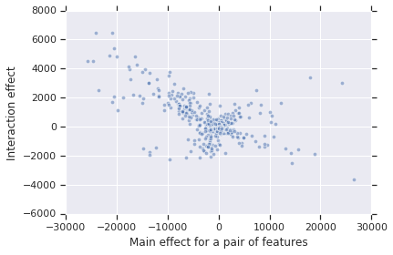
For the random forest regression task, we found that most of the influential pairwise feature interactions are substitutes; e.g. when the predicted price is lower than the average price, the main effects are negative, but the pair-wise interaction values are positive. We think this is because the features are correlated. We show a plot of main effects vs interaction effects of pairs of features in Figure 2.

For the reading comprehension task, previous analyses (cf. [16]) focused on whether the model ignored important question words. These analyses did not identify which paragraph words did the important question words match with. Our analysis identifies this. See the examples in Figure 3.


References
- [1] Aumann, R. J., and Shapley, L. S. Values of Non-Atomic Games. Princeton University Press, Princeton, NJ, 1974.
- [2] Baehrens, D., Schroeter, T., Harmeling, S., Kawanabe, M., Hansen, K., and Müller, K.-R. How to explain individual classification decisions. Journal of Machine Learning Research 11 (2009), 1803–1831.
- [3] Binder, A., Montavon, G., Lapuschkin, S., Müller, K.-R., and Samek, W. Layer-wise relevance propagation for neural networks with local renormalization layers. In ICANN (2016).
- [4] Cohen, S., Ruppin, E., and Dror, G. Feature selection based on the shapley value. In Proceedings of the 19th International Joint Conference on Artificial Intelligence (San Francisco, CA, USA, 2005), IJCAI’05, Morgan Kaufmann Publishers Inc., p. 665–670.
- [5] Cui, T., Marttinen, P., and Kaski, S. Recovering pairwise interactions using neural networks. CoRR abs/1901.08361 (2019).
- [6] Datta, A., Datta, A., Procaccia, A. D., and Zick, Y. Influence in classification via cooperative game theory. In Proceedings of the 24th International Conference on Artificial Intelligence (2015), IJCAI’15, AAAI Press, p. 511–517.
- [7] Datta, A., Sen, S., and Zick, Y. Algorithmic transparency via quantitative input influence: Theory and experiments with learning systems. 2016 IEEE Symposium on Security and Privacy (SP) (2016), 598–617.
- [8] Gelman, A., et al. Analysis of variance—why it is more important than ever. The annals of statistics 33, 1 (2005), 1–53.
- [9] Grabisch, M., and Roubens, M. An axiomatic approach to the concept of interaction among players in cooperative games. International Journal of Game Theory 28 (11 1999), 547–565.
- [10] Harrison, D., and Rubinfeld, D. L. Hedonic prices and the demand for clean air. J. Environ. Economics & Management 5 (1978), 81–102.
- [11] Kim, Y. Convolutional neural networks for sentence classification. In Proceedings of the 2014 Conference on Empirical Methods in Natural Language Processing, EMNLP 2014, October 25-29, 2014, Doha, Qatar, A meeting of SIGDAT, a Special Interest Group of the ACL (2014), A. Moschitti, B. Pang, and W. Daelemans, Eds., ACL, pp. 1746–1751.
- [12] Lundberg, S., and Lee, S.-I. A unified approach to interpreting model predictions. In NIPS (2017).
- [13] Lundberg, S. M., Erion, G. G., and Lee, S. Consistent individualized feature attribution for tree ensembles. CoRR abs/1802.03888 (2018).
- [14] Lundberg, S. M., and Lee, S.-I. A unified approach to interpreting model predictions. In Advances in Neural Information Processing Systems 30, I. Guyon, U. V. Luxburg, S. Bengio, H. Wallach, R. Fergus, S. Vishwanathan, and R. Garnett, Eds. Curran Associates, Inc., 2017, pp. 4768–4777.
- [15] Maleki, S., Tran-Thanh, L., Hines, G., Rahwan, T., and Rogers, A. Bounding the estimation error of sampling-based shapley value approximation with/without stratifying. ArXiv abs/1306.4265 (2013).
- [16] Mudrakarta, P. K., Taly, A., Sundararajan, M., and Dhamdhere, K. Did the model understand the question? In Proceedings of the 56th Annual Meeting of the Association for Computational Linguistics, ACL 2018, Melbourne, Australia, July 15-20, 2018, Volume 1: Long Papers (2018), I. Gurevych and Y. Miyao, Eds., Association for Computational Linguistics, pp. 1896–1906.
- [17] Owen, A. B. Sobol’ indices and Shapley value. SIAM Journal of Uncertainty Quantification 2, 1 (???? 2014), 245–251.
- [18] Owen, G. Multilinear extensions of games. Management Science 18, 5-part-2 (Jan. 1972), 64–79.
- [19] Precup, D., and Teh, Y. W., Eds. Proceedings of the 34th International Conference on Machine Learning, ICML 2017, Sydney, NSW, Australia, 6-11 August 2017 (2017), vol. 70 of Proceedings of Machine Learning Research, PMLR.
- [20] Rajpurkar, P., Zhang, J., Lopyrev, K., and Liang, P. Squad: 100, 000+ questions for machine comprehension of text. In Proceedings of the 2016 Conference on Empirical Methods in Natural Language Processing, EMNLP 2016, Austin, Texas, USA, November 1-4, 2016 (2016), pp. 2383–2392.
- [21] Shapley, L. S. A value of n-person games. Contributions to the Theory of Games (1953), 307–317.
- [22] Shrikumar, A., Greenside, P., and Kundaje, A. Learning important features through propagating activation differences. In Precup and Teh [19], pp. 3145–3153.
- [23] Simonyan, K., Vedaldi, A., and Zisserman, A. Deep inside convolutional networks: Visualising image classification models and saliency maps. CoRR (2013).
- [24] Singh, C., Murdoch, W. J., and Yu, B. Hierarchical interpretations for neural network predictions. In International Conference on Learning Representations (2019).
- [25] Sliwinski, J., Strobel, M., and Zick, Y. Axiomatic characterization of data-driven influence measures for classification. In The Thirty-Third AAAI Conference on Artificial Intelligence (2019), pp. 718–725.
- [26] Springenberg, J. T., Dosovitskiy, A., Brox, T., and Riedmiller, M. A. Striving for simplicity: The all convolutional net. CoRR (2014).
- [27] Strumbelj, E., and Kononenko, I. An efficient explanation of individual classifications using game theory. J. Mach. Learn. Res. 11 (Mar. 2010), 1–18.
- [28] Sundararajan, M., Taly, A., and Yan, Q. Axiomatic attribution for deep networks. In Precup and Teh [19], pp. 3319–3328.
- [29] Tibshirani, R. Regression shrinkage and selection via the lasso. Journal of the Royal Statistical Society: Series B (Methodological) 58, 1 (1996), 267–288.
- [30] Tsang, M., Cheng, D., and Liu, Y. Detecting statistical interactions from neural network weights. In International Conference on Learning Representations (2018).
- [31] Tsang, M., Liu, H., Purushotham, S., Murali, P., and Liu, Y. Neural interaction transparency (nit): Disentangling learned interactions for improved interpretability. In Advances in Neural Information Processing Systems 31, S. Bengio, H. Wallach, H. Larochelle, K. Grauman, N. Cesa-Bianchi, and R. Garnett, Eds. Curran Associates, Inc., 2018, pp. 5804–5813.
- [32] Yu, A. W., Dohan, D., Le, Q., Luong, T., Zhao, R., and Chen, K. Fast and accurate reading comprehension by combining self-attention and convolution. In International Conference on Learning Representations (2018).
6 Appendix
6.1 Proof of Theorem 1
Proof.
For a set , define the Möbius coefficients as:
Decomposition of any function into unanimity functions can be written in terms of ’s as follows:
Using the linearity axiom, we can extend from unanimity functions to as follows:
Using the Shapley-Taylor indices for unanimity functions from Proposition 4, we get:
Now we analyze the inner sum. We use the following identity: , where is the Beta function.
We use this expression for the inner sum in the above equation to get:
This finishes the proof. ∎
The next Lemma provides a relation between the Möbius coefficients and the discrete derivatives.
Lemma 2.
Möbius coefficients and discrete derivatives are related by following relation:
for and such that .
Proof.
Let and be two sets such that . We have
∎
6.2 Proof of Theorem 3
Proof.
Recall that for . First, we derive the multivariate expression in Equation 10.
Consider the expansion of :
Notice that is a multilinear function. Therefore, only the mixed partial terms survive. Furthermore, all mixed partials wrt are identical. Hence, we can simplify the above equation to:
Similarly, consider the multivariate Lagrange remainder term in Equation 10:
As before, in the derivative of , only the mixed partial terms are left:
We use this expression in Lagrange remainder term and interchanging the order of integral and summation. Note that there is an extra factor of that survives on the right side.
| (12) |
For the rest of the proof of the theorem, we consider the special case unanimity functions for a set and the corresponding multilinear extension:
| (13) |
We prove the theorem for the unanimity functions. Since unanimity functions form the basis, the general case follows from linearity axiom.
This proves the result for .
Next we analyze the Lagrange Remainder term. Consider a set . We use Eqaution 13 to evaluate :
| (15) | |||||
| ( if ) | |||||
| and | |||||
| is the Beta function | |||||
| from Equation 8 | |||||
This finishes the proof for the remainder term. ∎