Quantum transport through a coupled non-linear exciton-phonon system

Sima Pouyandeh^1,2,3, Hadi Z. Olyaei⁴ Affiliation: ¹Instituto de Telecomunicacoes, Physics of Information and Quantum Technologies Group, Portugal Affiliation: ²Instituto Superior Tecnico, Universidade de Lisboa, Portugal Affiliation: ³Centre de Biophysique Moleculaire, (CBM), CNRS UPR 4301, Rue C. Sadron, 45071, Orleans, France Affiliation: ⁴CeFEMA, Instituto Superior Técnico, Universidade de Lisboa, Av. Rovisco Pais, 1049-001 Lisboa, Portugal

Abstract

Wavepacket transport across a nonlinear region is studied numerically at zero and finite temperatures. In contrary to the zero temperature case which demonstrates ballistic transport, finite temperature lattice vibrations suppresses the transport drastically. The interface between the linear and the nonlinear chain plays the role of a high barrier at finite temperature when anharmonicity factor $\beta$ is small compared to the typical inverse cubic interatomic distance. Inverse participation ratio of the central region shows that for small anharmonicity and finite temperatures lattice vibrations give rise to self-trapping in the nonlinear chain which lasts for considerable times with a subdiffusive leakage of the wavepacket, almost equally, to both leads. The scenario changes when the anharmonicity becomes comparable with average inverse cubic interatomic distances as the lattice dynamics gives a profound boost to the transmission and starts to be almost transparent for the incoming pulse.

I Introduction

Nonlinear lattice dynamics is one of the pivotal subjects of modern condensed matter physics and nonlinear science. There has been enormous activity since the pioneering works of Fermi, Pasta, Ulam and Tsingou (Campbell et al. 2005; Gallavotti) for many years in the study of the spreading of wave packets known as energy excitations in numerous nonlinear models including the Fermi-Pasta-Ulam(FPU) model (Bourbonnais and Maynard 1990; Zavt et al. 1993; Leitner 2001; Snyder and Kirkpatrick 2006) and the discrete nonlinear Schrödinger equation(DNLSE)(Shepelyansky 1993; Molina 1998; Pikovsky and Shepelyansky 2008). Many experiments were performed within the context of wave packets spreading in nonlinear lattices with ultracold atomic condensates (Clément et al. 2006; Sanchez-Palencia et al. 2007; Billy et al. 2008; Lucioni et al. 2011), light energy transport in light-harvesting biomolecules and photosynthesis (van Amerongen et al. 2000; Blankenship 2002; Engel et al. 2007; Read et al. 2009; Collini et al. 2010; Romero et al. 2014).

Among various nonlinear models, DNLS effectively describes the dynamics of excitons interacting with lattice vibrations dynamics. The presence of nonlinearity in the DNLS keeps track of some interesting features in Bose-Einstein condensates BECs, (Xue and Zhang 2008; Wang et al. 2006) optical lattices, (Akhmediev et al. 2009; Ponomarenko and Agrawal 2006). Moreover, energy Localization or propagation of the stable solutions of DNLS, such as breathers and solitons, is associated to energy transfer in biological systems. (Braun and Kivshar 1998; Hennig and Tsironis 1999). There have been several investigations on the spreading of initially localized wave packets in a lattice with vibrations induced nonlinearity(Shepelyansky 1993; Kopidakis et al. 2008; Pikovsky and Shepelyansky 2008; Flach et al. 2009; Skokos et al. 2009; Mulansky and Pikovsky 2010; Laptyeva et al. 2010; Iomin 2010; Larcher et al. 2009; Iubini et al. 2015). The effect of nonlinearity on the transport features of disordered dynamical systems are also studied at length(Mulansky and Pikovsky 2010; Kopidakis et al. 2008; Flach 2010; García-Mata and Shepelyansky 2009; Mulansky and Pikovsky 2013; Ivanchenko et al. 2011). Vibrations induced nonlinearity gives rise to terms with cubic non-linearity in the DNLS equation which can be understood as an adiabatic-type approximation of phonon degrees of freedom(Chen et al. 1993; Molina and Tsironis 1993).

In this article, the adiabatic assumption is lifted by treating the lattice vibrations as a nonlinear FPU coupled with the Schrodinger equation governing the dynamics of the propagating wave packet. Hence, from the point of view of the expanding wave packet, the underlying lattice is a classical object which modifies the nearest neighbor hopping integrals and onsite potentials in the usual tight-binding approximation. The interplay between the quantum part(exciton) and the classical lattice, simulated as FPU chain, can significantly change electronic transport in the system. Studies on the coupled dynamical nature of exciton and underlying protein vibrations signify the role of vibrations modes in exciton energy transfer (O’Reilly and Olaya-Castro 2014; Tiwari et al. 2013; Mennucci and Curutchet 2011; Plenio and Huelga 2008; Lee et al. 2007; Wang et al. 2007; Adolphs and Renger 2006; Pouyandeh et al. 2017; Novo et al. 2016). Besides the fact that our grasp of energy spreading phenomenon in nonlinear lattices has enhanced over decades, there is still a universal mechanism missing in understanding the effect of out of equilibrium leads attached to the system is still open.

In this paper, we study energy transport through a nonlinear chain connected to two semi-infinite leads at its endpoints. The leads are regular linear one-dimensional lattices simulating the reflectionless contacts. The setup is of particular relevance for nano-bio-electronic devices. The central interest is to study the general features of energy/charge transport in such a device and to explore how an incident pulse travels through the nonlinear semiclassical lattice from a reservoir towards the central region. The configuration present in this paper takes also the linear/nonlinear interfaces into consideration as most semiconducting electronic devices have metallic tails with a minimum resistance and energy dissipation. So the linear/nonlinear interface plays a role of a dynamically varying barrier which needs to be taken into account.

In Sec. II we introduce the model describing the physical setup and the relevant tight-binding formulation along with the numerical method used to obtain the transmission. In Sec. III, includes some representative results of transmission and inverse participation ratio. In Sec. IV We conclude with a short summary. Sec. IV contains the details of obtaining semiclassical exciton-phonon coupling equations.

II Model and methods

Our system consists of two linear 1D chains serving as semi-infinite leads and a central region consisting of a finite length chain coupled to the underlying 1D classical lattice. The aim is to send a pulse from the left lead to the right to pass the non-linear chain as a barrier and study the transmission and reflection and other properties of this transport to get an insight for the behavior of this energy transport. In light-harvesting systems this pulse is, in fact, the wave function of an exciton, excited from a two-level quantum system of a pigment in a photosynthesis structure or a charge particle transporting in theses light-harvesting complexes. In this regard, we can investigate the role of non-linearity of the inter-atomic potentials underlying lattice as well as the role of local and non-local dynamical disorder in these complexes. The propagation of the pulse which is sent into the lattice and inherits a quantum nature together with the vibrations of the lattice are governed by the general following Hamiltonian

\displaystyle H

\displaystyle=

\displaystyle\sum_{{}_{mn}}J_{mn}\left(u_{m},u_{n}\right)B_{m}^{\dagger}B_{n}+\sum_{n}\frac{P_{n}^{2}}{2M}+\sum_{mn}V\left(u_{m},u_{n}\right)

Where $M$ is the bead mass, $B_{n}^{\dagger}$ , $B_{n}$ are creation and annihilation operators on site $n$ respectively and $u_{n}$ is the displacement of $n$ th bead with respect to its equilibrium position. In the Holstein model, the interaction of the quantum system with the lattice is defined by $J_{mm}=\epsilon_{m}+\chi u_{m}$ . In this model all the off-diagonal elements of $J_{mn}$ are set to zero except for the nearest neighbors ( $J_{m,m+1}=J_{m+1,m}=1$ ). In the so-called SSH (Su-Schrieffer-Heeger) model which is used mostly for the organic semiconductors the couplings are $J_{m,m+1}=J-\chi\left(u_{m}-u_{m+1}\right)$ and $J_{mm}=\epsilon_{m}$ (Su et al. 1979).

Here, we use a more physically realistic model which combines the two models. The Hamiltonian of an exciton propagating in the lattice is given by the tight-binding Hamiltonian

\displaystyle H_{e}

\displaystyle=

\displaystyle\sum_{n=1}^{L}\epsilon_{n}\left(u\right)B_{n}^{\dagger}B_{n}+\sum_{n=1}^{L}J_{n}\left(u\right)\left(B_{n+1}^{\dagger}B_{n}+B_{n}^{\dagger}B_{n+1}\right)

In which the effective interactions are modulated as following (Iubini et al. 2015)

$\displaystyle\epsilon_{n}$	$\displaystyle=$	$\displaystyle\epsilon_{0}+\chi_{E}\left(u_{n+1}-u_{n-1}\right)$	(3)
		,	(3)
$\displaystyle J_{n}$	$\displaystyle=$	$\displaystyle J_{0}+\chi_{J}\left(u_{n+1}-u_{n}\right)$	(4)

In the above equations $\epsilon_{0},J_{0}$ refer to the unperturbed values of site energies and hopping integrals respectively. Also, the parameters $\chi_{E},\chi_{J}$ are the strength of the exciton-lattice couplings.

Moreover, the Hamiltonian of the lattice which includes nonlinear interactions between nearest neighbor oscillators is given by

\displaystyle H_{l}

\displaystyle=

\displaystyle\sum_{n=0}^{L}\frac{p_{n}^{2}}{2M}+\frac{\kappa}{2}\left(u_{n+1}-u_{n}\right)^{2}+\frac{\beta}{4}\left(u_{n+1}-u_{n}\right)^{4}

(5)

Where, $\beta$ demonstrates the non-linearity of the lattice. In order to determine the evolution of the system, we obtain the equations of motion (EOM) for both quantum and classical parts. By defining a trial wave function for a single-exciton manifold $|\psi\left(t\right)\rangle=\sum_{n}b_{n}\left(t\right)B_{n}^{\dagger}|0\rangle$ and using it in the Schrodinger equation ( $i\hbar\frac{\partial}{\partial t}|\psi\left(t\right)\rangle=H|\psi\left(t\right)\rangle$ ) together with some identity relations we get the equation of motion of the exciton

\displaystyle i\hbar\frac{\partial}{\partial t}b_{j}\left(t\right)

\displaystyle=

\displaystyle\epsilon_{j}\left(u\right)b_{j}\left(t\right)+J_{j-1}\left(u\right)b_{j-1}\left(t\right)+J_{j}\left(u\right)b_{j+1}\left(t\right)

The EOM of the lattice will be that of a set of coupled oscillators driven by the exciton wave-function. From Newton’s law ( $M\ddot{u}_{n}=-\frac{\partial H}{\partial u_{n}}$ ), we can write:

$\displaystyle M\ddot{u}_{n}$	$\displaystyle=$	$\displaystyle-\frac{\partial}{\partial u_{n}}\langle\psi\|H\|\psi\rangle$	(7)
	$\displaystyle=$	$\displaystyle-\frac{\partial}{\partial u_{n}}\langle\psi\|H_{e}+H_{l}\|\psi\rangle$
	$\displaystyle=$	$\displaystyle F_{n}^{e}+F_{n}^{l}$

With $H_{e}$ and $H_{l}$ given in and 5 respectively.

Using Davydov trial wave function defined before, identity relations and normalization condition, after a few calculations similar to excitons, we obtain the EOM for the phonons as the classical part of the system

$\displaystyle M\ddot{u}_{n}$	$\displaystyle=$	$\displaystyle\kappa\left(u_{n+1}+u_{n-1}-2u_{n}\right)$	(8)
	$\displaystyle+$	$\displaystyle\beta\left[\left(u_{n-1}-u_{n}\right)^{3}+\left(u_{n+1}-u_{n}\right)^{3}\right]$
	$\displaystyle+$	$\displaystyle\chi_{E}\left(b_{n+1}^{}\left(t\right)b_{n+1}\left(t\right)-b_{n-1}^{}\left(t\right)b_{n-1}\left(t\right)\right)$
	$\displaystyle+$	$\displaystyle 2\chi_{J}Re\left(b_{n+1}^{}\left(t\right)b_{n}\left(t\right)-b_{n-1}^{}\left(t\right)b_{n}\left(t\right)\right)$

This equation together with the EOM of the exciton (Eq.) are integrated simultaneously by a fourth order Runge-Kutta method to determine the evolution of the coupled exciton-phonon non-linear system.

II.1 Initial and Boundary conditions

In order to investigate the energy transport in the system, we formulate the problem in terms of a localized wave packet moving towards a non-linear scattering region to get a motion picture displaying of reflection and transmission. We represent the initial state of the exciton by a Gaussian wave packet(Goldberg et al. 1967)

\displaystyle\psi(x,0)

\displaystyle=e^{ik_{0}x}e^{-(x-x_{0})^{2}/2\sigma_{0}^{2}}

(9)

This packet is centered around $x=x_{0}$ with a spread in $x$ dependent on $\sigma_{0}$ . The factor $e^{ik_{0}x}$ makes the wave function move to the right with average momentum $k_{0}$ . The choices of $x_{0}$ and $\sigma_{0}$ are governed by the boundary conditions and two more restrictions in the general situations which must be imposed in order that box normalization not give rise to difficulties. First of all, the packet is not allowed to travel so far that it hits the walls (Goldberg et al. 1967). For the total length of the system $L$ (including both leads and the non-linear chain), this restriction can be ensured by letting the center of the packet start from $L_{1}=x_{0}$ , move no farther to the right than $L_{2}$ , provided that the length of two leads is much larger than the chain. This can be accomplished by requiring that the average velocity of the wave packet be

\displaystyle k_{0}

\displaystyle\approx v_{0}=\frac{L_{2}-L_{1}}{T}

(10)

Where $T$ is the total time that is taken by the packet to move from $L_{1}$ to $L_{2}$ . In fact, the average momentum $k_{0}$ should be chosen in a way that the wave packet is transmitted through the chain fast enough without delocalization over the lead.

The second of the two restrictions concerns the fact that the reflected and transmitted packets must continue to be well enough localized so that at the end of the event they are out of the region of the potential and still far from the walls. It can be shown that if $\sigma_{0}$ is the initial spread in free space, then after a time $T$ the spread is given by(Goldberg et al. 1967)

\displaystyle\sigma^{2}

\displaystyle=\left(\sigma_{0}^{4}+4T^{2}\right)^{1/2}

(11)

Here we apply the same criteria for the spreading in the presence of a potential. For negligible spreading we must have $4T^{2}$ reasonably small compared with $\sigma_{0}^{4}$ .

However, despite these restrictions, as choosing long leads is time-consuming in terms of the numeric simulations, we have chosen another strategy to avoid the difficulties caused by wave packet when hitting the walls. Here we have applied absorbing boundary conditions at the walls in a way that we can make sure there will be no reflection from the walls so, the transmission that we calculate corresponds only to the initial pulse we had and not the reflected waves.

For the boundaries between leads and non-linear chain, we have chosen fixed boundary conditions which means that at the place where excitation hits scattering region the wave function should be zero at all times

\displaystyle\psi\left(N_{L}^{left},t\right)=\psi\left(N_{L}^{right},t\right)=0

(12)

Where $N_{L}^{left}$ , $N_{L}^{right}$ are the index of sites at right and left boundaries of the left and right leads with the lattice, respectively. This, of course, is applied to initial boundary conditions at $t=0$ for the same sites as well.

Figure 1 shows the exciton wave packet initially localized at $x_{0}$ for a system of total length 1000 with a non-linear lattice of 200 sites between two leads of length 400 each.We have chosen $x_{0}=350$ for the initial position of the pulse and $\sigma_{0}=10$ for spreading parameter which is $1\%$ of the total system length.

Refer to caption — Figure 1: Initial pulse localized at $x_{0}=N_{L}-50$ for a system of total length N=1000. The boundaries of leads and non-linear chain are specified by dashed lines. All the parameters including energies and couplings as well as non-linearity are kept one here.

Regarding the initial conditions for non-linear lattice, we suppose a characteristic configuration of the variables $u_{n}$ and $p_{n}$ representative of a finite temperature $T$ . This can be done by thermalizing the lattice via a Langevin heat bath at temperature $T$ for a sufficiently long transient time. For this, we implement a suitable friction term and a stochastic force to the free lattice EOMs (Iubini et al. 2015; Lepri 2003)

\displaystyle M\ddot{u}_{n}

\displaystyle=F_{n}^{l}-\gamma p_{n}+\sqrt{2\gamma T}\xi_{n}\left(t\right)

(13)

Where $\gamma$ is the coupling strength of the heat bath and $\xi_{n}\left(t\right)$ is a Gaussian white noise with correlation $\langle x_{i}\left(t\right)x_{i}\left(t^{\prime}\right)\rangle=2T\delta\left(t-t^{\prime}\right)$ . We start with a Maxwell distribution at temperature T for lattice configuration and then perturb momenta with random kicks extracted from a Gaussian distribution with $0$ mean and $2T\delta t$ variance. After the transient time $t_{0}$ we disconnect Langevin reservoir and integrate the equations of motion of the coupled system in order to study its transport properties.

III Results and Discussion

In this section, we study the process of energy transport through the chain. We study the exciton transfer in different regimes in terms of temperature, coupling strength and non-linearity. For that, we integrate the EOMs for both exciton and phonons (Eq. and Eq.8) simultaneously to treat the reflection-transmission event in a physical way. Later, we use our model to investigate the energy transport in an Organic semiconductor as a potentially natural light-harvesting system. Figure 2 shows the evolution of the initial excitonic pulse localized at $x_{0}=350$ over the whole system of total length $N=1000$ , with two leads of $N_{lead}=400$ each in the total time $t=40$ 0 at zero temperature. The initial width of pulse is $\sigma_{0}=10$ while all the other parameters including energies, couplings and non-linearity are kept one here.

We can see that in the case of zero temperature most part of the initial wave function is transferred through the non-linear chain. In the next part we will calculate the transmission and study its properties for different temperatures, non-linearity and coupling strengths.

III.1 Energy Transport

To gain insight into the process of energy transport, we study transmission and reflection phenomena and their relevance to other parameters of the system. Also to investigate the spread or localization of the exciton over lattice sites and get information in more details about its transfer, we obtain the participation ratio during different stages of the motion. The reflectivity and transmission probabilities are determined by recording and integrating the reflected and transmitted probability currents at $x=x_{r}$ and $x=x_{t}$ , two single positions before and beyond the scattering region, respectively. The integration must be performed over a duration spanning the entire scattering event (that is, waiting until the probability current has vanished at the single point). The transmission is (Dimeo 2014)

\displaystyle T

\displaystyle=\int_{0}^{t_{final}}dt^{\prime}j\left(x_{t},t^{\prime}\right)

(14)

Where, $j(x_{t},t^{\prime})$ is the probability current given by the usual definition

\displaystyle j(x,t)

\displaystyle=\frac{1}{2i}\left[\psi^{\star}\frac{\partial\psi}{\partial x}-\frac{\partial\psi^{\star}}{\partial x}\psi\right]

(15)

Similar to Eq. (14), reflection can be obtained, using

R=-\int_{0}^{t_{final}}dt^{\prime}j\left(x_{r},t^{\prime}\right)

(16)

Or, we can simply use Eq.(14) and calculate the reflection.

In our model of discrete lead and lattice sites, we have used the following probability current in discrete case

\displaystyle\jmath

\displaystyle=

\displaystyle i\sum_{i=1}^{N}J_{i}\left(b_{i}^{\star}b_{i+1}-b_{i+1}^{\star}b_{i}\right)

(17)

It is obtained directly from the quantum current flow $\jmath_{i}\text{=}i\left[H_{e},\hat{N_{i}}\right],\hbar=1$ for excitons, using identity relations and doing a bit of algebra.

In figure 3, the transmission is plotted in terms of temperature for two systems of total length $N=900$ and $N=1000$ with $N_{c}=100$ , $N_{c}=200$ over total transient time $t=700$ and $t=1000$ respectively. The length of leads in both systems is $N_{lead}=400$ each and the initial width of the pulse is $\sigma_{0}=10$ . All the other parameters including energies, couplings and non-linearity are kept one. The inset shows the logarithmic scale of the transmission over temperature for this system.

It is clear from the figures that by increasing temperature from zero, the transmission drops and then oscillates around small amounts. Here non-linear chain acts as an insulator which absorbs the energy of pulse, by reflecting and re-transmitting this energy from its boundaries several times inside the scattering region. However it seems that transport is slightly enhanced by increasing the temperature. But, in fact, it is due to the non-linearity properties of the system that in higher temperature lead to increase the amplitude of the osculations in the non-linear term and so slightly raise the average transport.

Figure 4 shows the density plot of wave function amplitude $|b|^{2}$ of the initial pulse during the evolution over all lattice sites of a system of total length $N=900$ with non-linear chain of length $N_{c}=100$ and two leads of length $N_{lead}=40$ 0 each for different temperatures. Figure 5 is density plot of pulse amplitude evolution only over non-linear lattice sites for the same temperatures as figure 4. As it is seen in the presence of temperature the pulse starts to spread over scattering region. In fact, at the higher temperatures the pulse even hardly reaches the second boundary and the transmission is almost zero.

To have a better insight into what happens inside this scattering region we have computed the inverse participation ratio (IPR) for different temperatures. IPR is a measure of localization and is defined as the average of the absolute value of the fourth power of the wave function. The maximum value of this quantity which is $IPR_{max}=1$ with a choice of normalization is reached when the wave function is completely localized while the minimum value is reached for a perfectly uniform state.

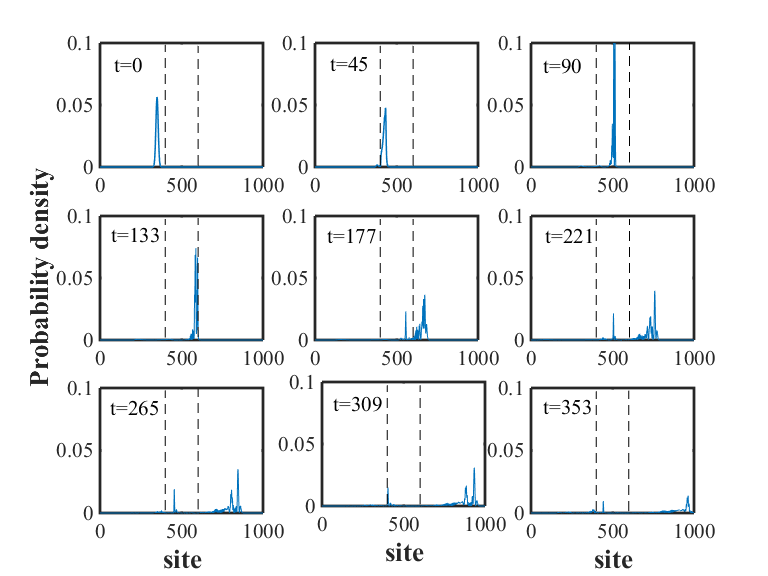
In figure 6 the evolution of IPR in the non-linear region is plotted at different temperatures for two systems of total length $900$ and $1000$ with $N_{c}=100$ , $N_{c}=200$ respectively while the length of each two leads in each system is $400$ . What is understood from these figures is that when the wave function reaches the scattering region, IPR goes up for a short time which means pulse is entering the region. However, this local wave function cannot keep its localization and spreads over lattice very fast. It is obvious that before the time that wave function reaches the region, IPR should be zero, however after entering the region, except for zero temperature it cannot keep higher values and before reaching the second boundary of non-linear region drops to zero which means that has lost its localization. Figure 7 shows the screenshot of the wave function amplitude over all lattice sites of the system with length 1000 for different temperatures at three times of entering the non-linear region, reaching the second boundary of this region and a time between these two times close to average maximum IPR.

However and despite this inefficient transport in the presence of temperature, surprisingly by increasing the non-linearity, transmission goes up. In figure 8 $a)$ and $b)$ we have plotted transmission in terms of the non-linearity parameter $\beta$ at three different temperatures for two systems of total length $900$ , $1000$ with non-linear chain of length $100$ , $200$ during the time evolution of $t=700$ and $t=1000$ respectively. As seen in this figure by increasing $\beta$ , transmission also increases and can reach up to $90\%$ for $T=1$ .

One explanation for this behavior could be hidden in the origin of coherence in the quantum transport systems such as photosynthetic complexes. In fact, it is experimentally and theoretically verified that the coherent exciton-vibrational (vibronic) coupling is of the origin of long-lasting coherence in the light-harvesting complexes both natural and artificial. Here, it can be concluded that the non-linearity is also another parameter of the origin of coherence among other parameters. However, what is seen here is that, non-linearity works as a catalyst for the whole system to improve quantum transport. In general, in a non-linear system there are two types of stable and unstable modes which can promote or demote the energy transport of the system. The normal modes will work as a repeater by creating recurrence and memory preserving of the modes while the unstable modes driven by instabilities caused by temperature will perturb the system in a destructive way. In other words, temperature and non-linearity play as rivals to prevent or promote the energy transport in the non-linear system. At lower temperatures the positive impact of non-linearity is more profound and as it is seen in figure 8 it can help transport to enhance up to 90 percent.

In figure 9 the effect of couplings between excitonic (pulse) and vibronic systems on transmission is also shown for the two systems of length $900$ , $1000$ with non-linear chain of length $100$ , $200$ during the time evolution of $t=700$ and $t=1000$ respectively. As expected, the most coupled the exciton is to the vibrations, the less it is free to move and so, the less the transmission is.

So, we can say that in one hand side, there are temperature and coupling strengths and on the other hand, non-linearity that interplay like rivals to help or harm the energy transport in the coupled exciton-phonon systems.

IV Conclusion

We numerically studied the quantum transport of the wavepacket across a nonlinear FPU chain. The results show that for small anharmonicity factors, finite temperature acts as an adverse control parameter in the transmission and causes self-trapping in the central region. Self-trapped wave leaks to the leads in a subdiffusive manner. Increasing the anharmonicity enhances transport significantly.

Acknowledgements.

S.P thanks the support from Fundaç

\tilde{a}

o para a Ci

\hat{e}

ncia e a Tecnologia (Portugal), namely through programme POCH and projects UID/EEA/50008/2013 and UID/EEA/50008/2019, as well as from the EU FP7 project PAPETS (GA 323901). Furthermore, H.Z.O and S.P acknowledge the support from the DP-PMI and FCT (Portugal) through scholarship PD/ BD/113649/2015 and PD/ BD/52549/2014 respectively. The authors kindly thank Yasser Omar, Francesco Piazza and Rui A. P. Perdigão for useful discussions related to this work.

References

Campbell et al. (2005) D. K. Campbell, P. Rosenau, and G. M. Zaslavsky, Chaos: An Interdisciplinary Journal of Nonlinear Science 15, 015101 (2005).
(2) G. Gallavotti, in The Fermi-Pasta-Ulam Problem (Springer Berlin Heidelberg, Berlin, Heidelberg) pp. 1–19.
Bourbonnais and Maynard (1990) R. Bourbonnais and R. Maynard, Physical Review Letters 64, 1397 (1990).
Zavt et al. (1993) G. S. Zavt, M. Wagner, and A. Lütze, Physical Review E 47, 4108 (1993).
Leitner (2001) D. M. Leitner, Physical Review B 64, 094201 (2001).
Snyder and Kirkpatrick (2006) K. A. Snyder and T. R. Kirkpatrick, Physical Review B 73, 134204 (2006).
Shepelyansky (1993) D. L. Shepelyansky, Physical Review Letters 70, 1787 (1993).
Molina (1998) M. I. Molina, Physical Review B 58, 12547 (1998).
Pikovsky and Shepelyansky (2008) A. S. Pikovsky and D. L. Shepelyansky, Physical Review Letters 100, 094101 (2008).
Clément et al. (2006) D. Clément, A. F. Varón, J. A. Retter, L. Sanchez-Palencia, A. Aspect, and P. Bouyer, New Journal of Physics 8, 165 (2006).
Sanchez-Palencia et al. (2007) L. Sanchez-Palencia, D. Clément, P. Lugan, P. Bouyer, G. V. Shlyapnikov, and A. Aspect, Physical Review Letters 98, 210401 (2007).
Billy et al. (2008) J. Billy, V. Josse, Z. Zuo, A. Bernard, B. Hambrecht, P. Lugan, D. Clément, L. Sanchez-Palencia, P. Bouyer, and A. Aspect, Nature 453, 891 (2008).
Lucioni et al. (2011) E. Lucioni, B. Deissler, L. Tanzi, G. Roati, M. Zaccanti, M. Modugno, M. Larcher, F. Dalfovo, M. Inguscio, and G. Modugno, Physical Review Letters 106, 230403 (2011).
van Amerongen et al. (2000) H. van Amerongen, R. van Grondelle, and L. Valkunas, Photosynthetic Excitons (WORLD SCIENTIFIC, 2000).
Blankenship (2002) R. E. Blankenship, ed., Molecular Mechanisms of Photosynthesis (Blackwell Science Ltd, Oxford, UK, 2002).
Engel et al. (2007) G. S. Engel, T. R. Calhoun, E. L. Read, T.-K. Ahn, T. Mancal, Y.-C. Cheng, R. E. Blankenship, and G. R. Fleming, Nature 446, 782 (2007).
Read et al. (2009) E. L. Read, H. Lee, and G. R. Fleming, Photosynthesis Research 101, 233 (2009).
Collini et al. (2010) E. Collini, C. Y. Wong, K. E. Wilk, P. M. G. Curmi, P. Brumer, and G. D. Scholes, Nature 463, 644 (2010).
Romero et al. (2014) E. Romero, R. Augulis, V. I. Novoderezhkin, M. Ferretti, J. Thieme, D. Zigmantas, and R. van Grondelle, Nature Physics 10, 676 (2014).
Xue and Zhang (2008) J.-K. Xue and A.-X. Zhang, Physical Review Letters 101, 180401 (2008).
Wang et al. (2006) B. Wang, P. Fu, J. Liu, and B. Wu, Physical Review A 74, 063610 (2006).
Akhmediev et al. (2009) N. Akhmediev, A. Ankiewicz, and J. M. Soto-Crespo, Physical Review E 80, 026601 (2009).
Ponomarenko and Agrawal (2006) S. A. Ponomarenko and G. P. Agrawal, Physical Review Letters 97, 013901 (2006).
Braun and Kivshar (1998) O. M. Braun and Y. S. Kivshar, Physics Reports 306, 1 (1998).
Hennig and Tsironis (1999) D. Hennig and G. Tsironis, Physics Reports 307, 333 (1999).
Kopidakis et al. (2008) G. Kopidakis, S. Komineas, S. Flach, and S. Aubry, Physical Review Letters 100, 084103 (2008).
Flach et al. (2009) S. Flach, D. O. Krimer, and C. Skokos, Physical Review Letters 102, 024101 (2009).
Skokos et al. (2009) C. Skokos, D. O. Krimer, S. Komineas, and S. Flach, Physical Review E 79, 056211 (2009).
Mulansky and Pikovsky (2010) M. Mulansky and A. Pikovsky, EPL (Europhysics Letters) 90, 10015 (2010).
Laptyeva et al. (2010) T. V. Laptyeva, J. D. Bodyfelt, D. O. Krimer, C. Skokos, and S. Flach, EPL (Europhysics Letters) 91, 30001 (2010).
Iomin (2010) A. Iomin, Physical Review E 81, 017601 (2010).
Larcher et al. (2009) M. Larcher, F. Dalfovo, and M. Modugno, Physical Review A 80, 053606 (2009).
Iubini et al. (2015) S. Iubini, O. Boada, Y. Omar, and F. Piazza, New Journal of Physics 17, 113030 (2015), arXiv:1505.03554 .
Flach (2010) S. Flach, Chemical Physics 375, 548 (2010).
García-Mata and Shepelyansky (2009) I. García-Mata and D. L. Shepelyansky, Physical Review E 79, 026205 (2009).
Mulansky and Pikovsky (2013) M. Mulansky and A. Pikovsky, New Journal of Physics 15, 053015 (2013).
Ivanchenko et al. (2011) M. V. Ivanchenko, T. V. Laptyeva, and S. Flach, Physical Review Letters 107, 240602 (2011).
Chen et al. (1993) D. Chen, M. I. Molina, and G. P. Tsironis, Journal of Physics: Condensed Matter 5, 8689 (1993).
Molina and Tsironis (1993) M. I. Molina and G. P. Tsironis, Physical Review B 47, 15330 (1993).
O’Reilly and Olaya-Castro (2014) E. J. O’Reilly and A. Olaya-Castro, Nature Communications 5, 3012 (2014).
Tiwari et al. (2013) V. Tiwari, W. K. Peters, and D. M. Jonas, Proceedings of the National Academy of Sciences of the United States of America 110, 1203 (2013).
Mennucci and Curutchet (2011) B. Mennucci and C. Curutchet, Physical Chemistry Chemical Physics 13, 11538 (2011).
Plenio and Huelga (2008) M. B. Plenio and S. F. Huelga, New Journal of Physics 10, 113019 (2008).
Lee et al. (2007) H. Lee, Y.-C. Cheng, and G. R. Fleming, Science (New York, N.Y.) 316, 1462 (2007).
Wang et al. (2007) H. Wang, S. Lin, J. P. Allen, J. C. Williams, S. Blankert, C. Laser, and N. W. Woodbury, Science (New York, N.Y.) 316, 747 (2007).
Adolphs and Renger (2006) J. Adolphs and T. Renger, Biophysical Journal 91, 2778 (2006).
Pouyandeh et al. (2017) S. Pouyandeh, S. Iubini, S. Jurinovich, Y. Omar, B. Mennucci, and F. Piazza, Physical Biology 14, 066001 (2017).
Novo et al. (2016) L. Novo, M. Mohseni, and Y. Omar, Scientific Reports 6, 18142 (2016), arXiv:1312.6989 .
Su et al. (1979) W. P. Su, J. R. Schrieffer, and A. J. Heeger, Physical Review Letters 42, 1698 (1979).
Goldberg et al. (1967) A. Goldberg, H. M. Schey, and J. L. Schwartz, Am. J. Phys. 35, 177 (1967).
Lepri (2003) S. Lepri, Physics Reports 377, 1 (2003).
Dimeo (2014) R. M. Dimeo, American Journal of Physics 82, 142 (2014).