Self-adaptive Single and Multi-illuminant Estimation Framework
based on Deep Learning
Abstract
Illuminant estimation plays a key role in digital camera pipeline system, it aims at reducing color casting effect due to the influence of non-white illuminant. Recent researches shi2016deep, hu2017fc handle this task by using Convolution Neural Network (CNN) as a mapping function from input image to a single illumination vector. However, global mapping approaches are difficult to deal with scenes under multi-light-sources. In this paper, we proposed a self-adaptive single and multi-illuminant estimation framework, which includes the following novelties: (1) Learning local self-adaptive kernels from the entire image for illuminant estimation with encoder-decoder CNN structure; (2) Providing confidence measurement for the prediction; (3) Clustering-based iterative fitting for computing single and multi-illumination vectors. The proposed global-to-local aggregation is able to predict multi-illuminant regionally by utilizing global information instead of training in patches bianco2015single gijsenij2012color, as well as brings significant improvement for single illuminant estimation. We outperform the state-of-the-art methods on standard benchmarks with the largest relative improvement of 16%. In addition, we collect a dataset contains over 13k images for illuminant estimation and evaluation. The code and dataset is available on https://github.com/LiamLYJ/KPF_WB.
| Input | Clustering | Local Fitting | GT | FC4 hu2017fc |

1 Introduction
In recent years, there has been a considerable growth in digital cameras market. Illuminant estimation is one of the core factors to improve the quality of captured photographs. It is responsible for adjustment of the intensities of colors, typically in primary colors: red, green and blue. The goal of illuminant estimation is to render the neutral colors (the colors under white light source) correctly under non-white light sources. Hence, general method in a camera pipeline system has an alias of “White Balance” (WB). Apart from photography, a lot of computer vision tasks are based on extracting comprehensive information from the intrinsic colors of objects, e.g. image segmentation, object recognition, etc.
Unlike Human Visual System (HVS), which can automatically compensate for the illumination effect of color perception by adjusting the photoreceptors with our brain, a digital camera system needs to estimate the environment illuminant accurately in order to retrieve the intrinsic color. Human eyes are good at judging the intrinsic color under different light sources because of the color constancy being memoried by the biological vision system (in the V4 cells khalil2015biologically). HVS involves both photo-receptors and neurons in eyes, and contains additional complex processing in our brain. We memorize what objects are supposed to be in color under different environments, and perform corresponding adjustment subconsciously. However, digital cameras often have difficulty on performing similar adjustment, i.e. “Auto White Balance” (AWB). This is mainly caused by the illuminant tint influence, which usually affects image sensor directly. An accurate illuminant estimation method, aiming at correct compensation for photosensitive devices, is needed to handle wide range of light conditions. The old-school style of camera AWB is implemented in a similar way as HVS, in the form of “matrix metering” by recording scene information into a prepared database. However, the traditional way involves a lot of manual efforts and performs badly in complex illumination environment. For example, indoor environment usually has multi-illuminant with complicated reflections, which makes it almost impossible to be labeled.
2 Related Work
There are many traditional methods try to determine the color of objects under the canonical illuminant with specific assumptions. Different assumptions have given rise to numerous illuminant estimation methods that can be divided into two main groups. First of these groups contains low-level statistic based methods, such as White-patch brainard1986analysis, Gray-world buchsbaum1980spatial, Shades-of-Gray finlayson2004shades, Grey-Edge (1st and 2nd order) van2007edge, using the bright pixels joze2012role, etc. The second group includes machine-learning based methods, such as gamut mapping (pixel, edge, and intersection based) barnard2000improvements, natural image statistics gijsenij2011color, Bayesian learning gehler2008bayesian, spatio-spectral learning (maximum likehood estimation) chakrabarti2012color, using color/edge moments finlayson2013corrected, using regression trees with simple features from color distribution cheng2015effective and performing various kinds of spatial localizations barron2015convolutional, DBLP:journals/corr/BarronT16.
These assumptions based methods brainard1986analysis, buchsbaum1980spatial, finlayson2004shades, van2007edge, joze2012role, etc, usually perform badly when there are no white patches in the scene. e.g. scene with large area of green grass or blue sea. The current industrial way of implementing AWB algorithms is based on combining statistic-based methods with feature learning. The approach mainly consists of: (1) scene recognition, (2) estimation under different scene battiato2012instant.
Because of the outstanding learning performance on various computer vision tasks based on CNN compared with traditional machine learning methods, the state-of-the-art single illuminant estimation techniques bianco2015color, lou2015color, shi2016deep, hu2017fc, DBLP:journals/corr/BarronT16, bianco2015single, gijsenij2012color harness the power of CNN to train illuminant estimation models using large training sets composed of minimally processed images (linear RGB image generated from RAW) and their associated labels of single illumination vector. bianco2015color operates on sampled image patches as input, uses a CNN structure consists of convolutional layer, max pooling, fully connected layer and three output nodes for illumination vector. lou2015color proposes a framework using CNN to obtain more accurate light source estimation. They reformulate illuminant estimation as a CNN-based regression problem. shi2016deep proposes a CNN architecture with two interacting sub-networks, i.e. a hypotheses network (HypNet) and a selection network (SelNet) for better performance. hu2017fc presents a fully convolutional network architecture with confidence-pooling layer which is able to determine “what to learn” and “how to pool” automatically from training data. FFCC DBLP:journals/corr/BarronT16 reformulates the problem of color constancy as a 2D spatial localization task in a log-chrominance space, and proceeds Bivariate Von Mises (BVM) estimation procedure on the frequency domain. Especially, they use camera meta-data (e.g. shutter speed) as extra semantic features to train a CNN model with better performance.
Other techniques like bianco2015color, lou2015color, shi2016deep, hu2017fc, etc aim at using deep CNN to extract high level feature for illuminant estimation, and they consider CNN as a “black box” global mapping function directly map the input image to its corresponding illumination vector. In this paper, we present a CNN architecture for generating a local-based self-adaptive meaningful kernel for its own input. The illumination vector will be calculated based on the refrence image computed by applying the learned kernel on its input image.
Certainly, the “no white patch” case can be solved by CNN based techniques because of its data-driven property. e.g., if training data contain enough green grass scene, the model will learn to predict correctly for similar green scene. However, more often than not, the assumption of a uniform illuminant is an insufficient approximation under real-world illumination conditions (multiple light sources, shadows, interreflections, etc). riess2011illuminant presents a physics-based approach for illuminant color estimation of arbitrary images, which is explicitly designed for handling images with multiple illuminants. Its building block is the computation of statistically robust local illuminant estimates which are then used in deriving the number and color of the dominant illuminants. beigpour2014multi formulates the multi-illuminant estimation problem as an energy minimization task within a Conditional Random Field over a set of local illuminant estimates. bianco2015single and gijsenij2012color propose a similar methodology to extend existing algorithms by producing corresponding local estimation with image patches rather than using the entire image. gijsenij2012color combines local patch estimations based on a modified diagonal model, bianco2015single trains a non-linear mapping based on radial basis function kernel over local statistics of local estimations as a local-to-global regressor. Techniques similar to riess2011illuminant, beigpour2014multi, gijsenij2012color, bianco2015single, etc manage multi-illuminant problem into two stages: (1) split input image into local patches, then estimate on these patches isolatedly; (2) combine the local estiamtions in a super-pixel level. However, local estimations make more sense when it is driven from global information, and less accurate when only from its restricted local information.
The rest of this paper is organized as following: Section 3 formalizes the illuminant estimation problem and illustrates our proposed framework in detail. Section 4 describes the dataset and experimental results along with evaluation. We demonstrate the proposed method on four benchmarks and reach the largest relative improvement of 16% compare to the state-of-the-art method. In Section 5, we present a summary and discussion of possible future works.
3 Proposed Framework
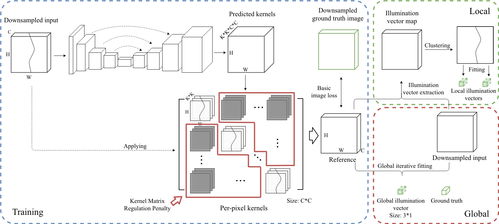
In this paper, we present a framework to estimate single and multi-illuminant based on fully convolutional neural network, local illuminant is estimated from the whole image instead of patches as in works like riess2011illuminant, beigpour2014multi, gijsenij2012color, bianco2015single, etc. Also different from other works bianco2015color, lou2015color, shi2016deep, hu2017fc, etc which directly map input image into its corresponding illumination vector, we use CNN to learn an explicable kernel. The proposed global-to-local aggregation framework (see Figure 2) includes:
- 1.
An encoder-decoder CNN structure to learn local self-adaptive kernels from global information.
- 2.
Confidence measurement based on the learned kernels and its input image.
- 3.
Clustering based iterative fitting for computing single and multi-illumination vectors subregionally.
Each of these three stages will be explained in detail in the following subsections.
3.1 Problem Formulation
The aim of illuminant estimation is to transform image captured under unknown light sources into a color-balanced one, as if they appear under the canonical illuminant. Usually, this is done by using a diagonal model:
| (1) |
where is the image taken under unknown illuminant environment, is the transformed image appears as if it is taken under the canonical illuminant. The is the transform diagonal matrix which takes the following form:
| (2) |
where is unknown illuminant and is canonical illuminant. For AWB module in camera pipeline, , , , usually alias , , respectively.
AWB requires an automatically channel wised correction based on the prediction of illuminant color. Since here we might need different gain values for different objects or different illuminant situations, we expect CNN structure to tackle this problem.
3.2 Self-adaptive Kernel Learning
The design of proposed CNN network architecture aims to directly use the pixel-wise information from the input image, with the minor concern of extracting the high-level feature. In this paper, we use the CNN architecture in encoder-decoder design with skip connections. Such architecture has been proved to be efficient in various pixel-level applications. For example, “U-net” structure for image segmentation DBLP:journals/corr/RonnebergerFB15, image to image pixel wise translation isola2017image, image denoising from a burst of input images DBLP:journals/corr/abs-1712-02327.
Unlike works DBLP:journals/corr/RonnebergerFB15, isola2017image try to synthesize the output image pixels using this architecture, in this paper, we use it for learning local self-adaptive kernels from global information. Instead of directly using CNN to predict illumination vector, we tackle this problem by first learn a intermediate mutable function i.e. self-adaptive kernels, final prediction of illumination vector will be computed based on learned spatial variant kernels and corresponding input. Such global-to-local aggregation brings significant improvement to the single illuminant estimation and better addresses multi-source illumination problem as well as extracting confidence measurement.
Considering the usage of channel-wise correction in WB task, we first try predicting kernel maps (with the same size as downsampled input image) separately for each channel: kernel maps ( for a single RGB image) with (K-order, kernel) channels for each pair of input-output channels. The value at each pixel in each output channel of reference image will be computed as pixel-wise dot product as following:
| (3) |
where denotes the neighbourhood of pixel in each input channel , and is its corresponding kernel. Such design of spatial adaptive kernel aims at enhancing local illuminant estimation from global information instead of treating image patches independently (Figure 2).
Moreover, in order to make fully use of image information, we propose computing additional kernels for cross-channel operations, which yields better performance in our experiments. We compute kernel maps with channels, and the reference output is obtained by applying the learned kernels across all channels:
| (4) |
This adjustment favors the learning in two ways: (1) It increases the model complexity without deepening the network structure. (2) It compensates the insufficient optimization when channel wise-information is not rich enough. This cross-channel approach achieve the best results in all following experiments.
The loss function we used to learn the kernels consists of two parts: the basic image loss similar to the loss function in DBLP:journals/corr/abs-1712-02327, and the additional kernel matrix regulation penalty to encourage kernels to utilize corresponding channel information more.
The basic image loss is a weighted average of L2 distance on pixel intensities and L1 distance on pixel gradients as compared to the ground truth image, which is obtained by applying accordingly ground truth illumination vector on the input image. We apply the loss after applying the sRGB transfer function for gamma correction, which can produce a more perceptually relevant estimation DBLP:journals/corr/abs-1712-02327. The basic L1 and L2 image loss are shown as:
| (5) |
Where is the finite difference operator that convolves its input with and , and denote for the sRGB transformation for both input and output channel:
| (6) |
where and denotes for linear input channel , , or .
Apart from image loss, we introduce L1 kernel matrix regulation penalty during training (Equation 7). This penalty punishes the kernels that do not align with the same input and output channel. The intuition is: although we utilize cross-channel information, we expect the learned kernels still focus on the corresponding channel due to the channel-wise property persevering in WB training dataset. The proposed L1 kernel matrix regulation penalty forms as following:
| (7) |
Our final loss function forms as following:
| (8) |
where denotes for applying the learned kernel on the input image as Equation 4, loss weights of , and are set to respectively in our experiments.
By applying learned kernels to downsampled input image, we get a reference image. The final illumination vector is produced by iterative fitting using the reference image as described in subsection 3.4. In addition, prediction confidence can be derived by learned kernels (subsection 3.3), thereby the proposed method offers much more freedom for further hand-engineered calibration as well as following stages in camera image processing pipeline.
3.3 Confidence Estimation
As mentioned before, we predict kernels from downsampling resized input image. Such “kernel matrix” form enables that each input channels can contribute to output channels. Due to the channel-wise property in WB task as well as our kernel matrix regulation penalty, we define the confidence value to be the rate between the “contribution” from the corresponding input channel and the others.
Confidence value for each channel in pixel is defined as following:
| (9) |
By combining confidence across all channels, we can get a uniformed estimation. The empirical evidence shows that confidence value is proportional to the mean of all confidence maps, and inversely proportional to the variance of all confidence maps:
| (10) |

3.4 Iterative Fitting and Illuminant Clustering
We adopt clustering and iterative fitting to solve illumination vector subregionally. The goal of iterative fitting is to find optimal gain values to make the white balanced image close to the reference in general. The segmental workflow benifits in two parts compare with directly applying kernels on original input image: First, for high-resolution images (e.g. 4K images), the downsample resizing operation save the hardware cost; Second, the iterative fitting method will compress the artifacts occur in underexposure region due to the spikes in illuminant vector map. The example of artifacts coming from directly applying kernels is shown in Figure 3. In the column of kernel applying, the artifacts appear at the over dark region of lower right corner (last row).
In WB task, the fitting target is three dimensional vector (Equation 1). We minimize the L2 distance between the reference image and the fitting results image :
| (11) |
where is computed using the fitting target.
Due to the limited complexity of fitting target we used downhill simplex algorithm nelder1965simplex with the initialization gain value as constant 1.0 in our experiment, which works well in our evaluations. Further improvement may be acquired by using more powerful optimization methods.
However, uniform illuminant assumption is insufficient for real-world applications. Instead of using global fitting, we divide the input image into subregions that vary by different illuminants. Specifically, for each input-reference pair, an illumination vector map could be acquired by the division between reference and input, the clustering is performed on the illumination vector map.
Considering the specific of illuminant clustering (few cluster number, non-flat geometry), we select Spectral Clustering (SC) stella2003multiclass in our following experiments. SC requires the number of clusters to be specified, in our experiments we set to 2. For two clusters, it solves a convex relaxation of the normalized cuts problem on the similarity graph: cutting the graph in two so that the weight of the edges cut is small compared to the weights of the edges inside each cluster. In our case, graph vertices are defined as each pixel on the illumination vector map, and edges are defined as the similarity between two illumination vector modeled by RBF kernel: , where is the parameter to control kernel variance, and the distance between and is computed as vectors angle distance:
| (12) |
In order to show the adaptive performance on multi-illuminance circumstance, we concatenate two image parts that under different illumination into one image. The clustering and fitting result on the concatenated images are shown in Figure 3 at local fitting column. From the result, we could see improvements on local illuminant estimation compare to global fitting.
4 Experimental Results
We present the implementation and training detail in Section 4.1. Quantitative evaluations of the proposed method on benchmarks are given in Section 4.2, including open source benchmarks (Gehler gehler2008bayesian, NUS-8 cheng2014illuminant and one self-collected dataset captured by Sony DSC-RX100M3 single-lens reflex(DSLR) camera. See supplement for more experiments and results. A gamma correction of on linear RGB images is applied for display. Further detail is presented in Section 4.3.
4.1 Implementation and Training
Our proposed network architecture is implemented by Tensorflow 22 2 https://www.tensorflow.org/, network architecture is shown in Figure 2, ReLu is used for non-linear activation except for the final layer. We deploy variants of network architecture with different input size and filter size for evaluating our method, our best results is from structure of with input size , filter size . Moreover, benefit from our efficient design of network architecture, the architecture with input size , filter size and also exhibit the comparable performance which require much less computational cost (see supplement), e.g. hu2017fc uses as input. We apply the following data augmentation: Randomly crop of the images, which are initially obtained by first randomly choosing a side length that is 0.1 to 0.9 times the shorter edge of the original image; Randomly rotation between -60 to 60 degree; Randomly left-right top-down flip with a probability of 0.5; Randomly divide and concatenate two input image together for one new training sample. After augmentation, image will be resized into according input size. We use Adam kingma2014adam optimization algorithm with batch size of 32 and a base learning rate of . The training runs one million iterations on an NVIDIA 1080Ti GPU and takes 3 days in our setting. Our code will be made available publicly.
| Method | Mean | Med. | Tri. |
|
|
G.M. | ||||
|---|---|---|---|---|---|---|---|---|---|---|
| White-Patch brainard1986analysis | 7.55 | 5.68 | 6.35 | 1.45 | 16.12 | 5.76 | ||||
| Gray-World buchsbaum1980spatial | 6.36 | 6.28 | 6.28 | 2.33 | 10.58 | 5.73 | ||||
| Edge-based Gamut barnard2000improvements | 6.52 | 5.04 | 5.43 | 1.90 | 13.58 | 5.40 | ||||
| 1st-order Gray-Edge van2007edge | 5.33 | 4.52 | 4.73 | 1.86 | 10.03 | 4.63 | ||||
| 2nd-order Gray-Edge van2007edge | 5.13 | 4.44 | 4.62 | 2.11 | 9.26 | 4.60 | ||||
| Shades-of-Gray finlayson2004shades | 4.93 | 4.01 | 4.23 | 1.14 | 10.20 | 3.96 | ||||
| Bayesian gehler2008bayesian | 4.82 | 3.46 | 3.88 | 1.26 | 10.49 | 3.86 | ||||
| General Gray-World barnard2002comparison | 4.66 | 3.48 | 3.81 | 1.00 | 10.09 | 3.62 | ||||
| Spatio-spectral Statistic chakrabarti2012color | 3.59 | 2.96 | 3.10 | 0.95 | 7.61 | 2.99 | ||||
| Interesection-based Gamut barnard2000improvements | 4.20 | 2.39 | 2.93 | 0.51 | 10.70 | 2.76 | ||||
| Pixels-baed Gamut barnard2000improvements | 4.20 | 2.33 | 2.91 | 0.50 | 10.72 | 2.73 | ||||
| Cheng et al.2014 cheng2014illuminant | 3.52 | 2.14 | 2.47 | 0.50 | 8.74 | 2.41 | ||||
| Exemplar-based joze2014exemplar | 2.89 | 2.27 | 2.42 | 0.82 | 5.97 | 2.39 | ||||
| Corrected-Moment finlayson2013corrected | 2.86 | 2.04 | 2.22 | 0.70 | 6.34 | 2.25 | ||||
| Bianco CNN bianco2015color | 2.63 | 1.98 | 2.10 | 0.72 | 3.90 | 2.04 | ||||
| Cheng et al. 2015 cheng2015effective | 2.42 | 1.65 | 1.75 | 0.38 | 5.87 | 1.73 | ||||
| CCC barron2015convolutional | 1.95 | 1.22 | 1.38 | 0.35 | 4.76 | 1.40 | ||||
| DS-Net shi2016deep | 1.90 | 1.12 | 1.33 | 0.31 | 4.84 | 1.34 | ||||
| SqueezeNet-FC4 hu2017fc | 1.65 | 1.18 | 1.27 | 0.38 | 3.78 | 1.22 | ||||
| FFCC DBLP:journals/corr/BarronT16 | 1.61 | 0.86 | 1.02 | 0.23 | 4.27 | 1.07 | ||||
| Our method | 1.35 | 0.76 | 0.98 | 0.22 | 3.76 | 0.93 |
4.2 Benchmark Evaluation
We evaluate the proposed framework on three open source benchmarks: Gehler gehler2008bayesian, NUS-8 cheng2014illuminant and Cube DBLP:journals/corr/abs-1712-00436 (see supplement for Cube dataset). The Gehler dataset contains 568 images with both indoor and outdoor shots taken by two high quality digital DSLR cameras (Canon 5D and Canon1D) with all settings in auto mode. 482 images for camera Canon 5D and 84 images for camera Canon 1D. NUS-8 dataset contains total number of 1736 images captured by 8 different cameras: Canon EOS-1Ds Mark III, Canon EOS 600D, Fujifilm X-M1, Nikon D5200, Olympus E-PL6, Panasonic Lumix DMC-GX1, Samsung NX2000, and Sony SLT-A57. There are roughly equal numbers of images for each camera. We split the datasets into 5 folds, and perform cross evaluating on four of five for training and remaining for testing. Several standard metrics are reported in terms of angular distance with ground truth (see Equation 12, in degree) : mean, median, tri-mean of all the errors, mean of the lowest 25% of errors, and mean of the highest 25% of errors.
For images in Gehler and NUS-8 datasets, a Macbeth ColorChecker (MCC) is presented for obtaining the ground truth illumination vector. The ground truth is obtained from the difference between the two brightest achromatic patches containing no saturated value to get rid of the effects from the dark level and saturation level of the sensor. In order to use those images, dark level has to be subtracted from the original images which is provided in the ground truth files from these datasets. Table 1 and Table 2 summarize the results of our proposed method based on global fitting and previous algorithms on Gehler and NUS-8 dataset. Notice that we reach the relative improvement around 16% on Gehler dataset compare to state-of-the-art algorithm DBLP:journals/corr/BarronT16, and small improvement on NUS-8 datasets. We argue the reason is that the diverse optical characteristic among different camera results in making the distribution of input data dispersive which increase learning difficulty inevitably. The supplement contains additional results on Cube DBLP:journals/corr/abs-1712-00436 dataset.
| Method | Mean | Med. | Tri. |
|
|
G.M. | ||||
|---|---|---|---|---|---|---|---|---|---|---|
| White-Patch brainard1986analysis | 10.62 | 10.58 | 10.49 | 1.86 | 19.45 | 8.43 | ||||
| Edge-based Gamut barnard2000improvements | 8.43 | 7.05 | 7.37 | 2.41 | 16.08 | 7.01 | ||||
| Pixels-baed Gamut barnard2000improvements | 7.70 | 6.71 | 6.90 | 2.51 | 14.05 | 6.60 | ||||
| Interesection-based Gamut barnard2000improvements | 7.20 | 5.96 | 6.28 | 2.20 | 13.61 | 6.05 | ||||
| Gray-World buchsbaum1980spatial | 4.14 | 3.20 | 3.39 | 0.90 | 9.00 | 3.25 | ||||
| Bayesian gehler2008bayesian | 3.67 | 2.73 | 2.91 | 0.82 | 8.21 | 2.88 | ||||
| Natural Image Statics gijsenij2011color | 3.71 | 2.60 | 2.84 | 0.79 | 8.47 | 2.83 | ||||
| Shades-of-Gray finlayson2004shades | 3.40 | 2.57 | 2.73 | 0.77 | 7.41 | 2.67 | ||||
| General Gray-World barnard2002comparison | 3.21 | 2.38 | 2.53 | 0.71 | 7.10 | 2.49 | ||||
| 2nd-order Gray-Edge van2007edge | 3.20 | 2.26 | 2.44 | 0.75 | 7.27 | 2.49 | ||||
| Bright Pixels joze2012role | 3.17 | 2.41 | 2.55 | 0.69 | 7.02 | 2.48 | ||||
| 1st-order Gray-Edge van2007edge | 3.20 | 2.22 | 2.43 | 0.72 | 7.36 | 2.46 | ||||
| Spatio-spectral Statics chakrabarti2012color | 2.96 | 2.33 | 2.47 | 0.80 | 6.18 | 2.43 | ||||
| Corrected-Moment finlayson2013corrected | 3.05 | 1.90 | 2.13 | 0.65 | 7.41 | 2.26 | ||||
| Color Tiger DBLP:journals/corr/abs-1712-00436 | 2.96 | 1.70 | 1.97 | 0.53 | 7.50 | 2.09 | ||||
| Cheng et al. 2014 cheng2014illuminant | 2.92 | 2.04 | 2.24 | 0.62 | 6.61 | 2.23 | ||||
| Color Dog banic2015color | 2.83 | 1.77 | 2.03 | 0.48 | 7.04 | 2.03 | ||||
| DS-Net shi2016deep | 2.24 | 1.46 | 1.68 | 0.48 | 6.08 | 1.74 | ||||
| CCC barron2015convolutional | 2.38 | 1.48 | 1.69 | 0.45 | 5.85 | 1.74 | ||||
| SqueezeNet-FC4 hu2017fc | 2.23 | 1.57 | 1.72 | 0.47 | 5.15 | 1.71 | ||||
| Cheng et al. 2015 cheng2015effective | 2.18 | 1.48 | 1.64 | 0.46 | 5.03 | 1.65 | ||||
| FFCC DBLP:journals/corr/BarronT16 | 1.99 | 1.31 | 1.43 | 0.35 | 4.75 | 1.44 | ||||
| Our method | 1.96 | 1.41 | 1.44 | 0.35 | 4.29 | 1.36 |
In addition to the open source benchmarks, we provide evaluation on a self-collected dataset named MIO (massive-indoor-outdoor) dataset. It contains massive indoor and outdoor images (over 13k) captured by Sony DSC-RX100M3 camera. The ground truth is obtained based on the meta-file generated by DSC-RX100M3 camera. The goal of collecting such a dataset aims at evaluating the performance of an AWB algorithm to the maximum close to real world application instead of making benchmark for training with accurate ground truth. We split the training, validation and test sets as 9k, 2k, 2k images. We only do minimal processing on the resolution of 4864x3648 (4:3) raw images to get linear training images as same as on Gehler gehler2008bayesian and NUS-8 cheng2014illuminant datasets. The dataset contains both outdoor images and indoor images in parts of Tokyo and ShengZhen under various seasons. Especially, it contains multiple corner case scene which traditional camera algorithm performs badly on. e.g. full scene with green grass, human skin in indoor (2500-3000K). Table 3 exhibits the performance of proposed methods and other methods on MIO dataset, we outperform state-of-the-art algorithm in all the evaluation metrics.
| Method | Mean | Med. | Tri. |
|
|
G.M. | ||||
|---|---|---|---|---|---|---|---|---|---|---|
| White-Patch brainard1986analysis | 5.59 | 4.42 | 5.21 | 1.09 | 15.25 | 4.28 | ||||
| Gray-world buchsbaum1980spatial | 3.75 | 2.95 | 3.18 | 0.89 | 9.02 | 2.89 | ||||
| Shades-of-Gray finlayson2004shades | 2.61 | 1.72 | 1.96 | 0.47 | 8.01 | 1.91 | ||||
| 1st-order Gray-Edge van2007edge | 2.47 | 1.61 | 1.89 | 0.43 | 6.32 | 1.90 | ||||
| 2nd-order Gray-Edge van2007edge | 2.46 | 1.59 | 1.91 | 0.45 | 6.19 | 1.89 | ||||
| Bright Pixels joze2012role | 2.42 | 1.57 | 1.84 | 0.46 | 5.99 | 1.89 | ||||
| FFCC DBLP:journals/corr/BarronT16 | 1.09 | 0.81 | 0.82 | 0.30 | 1.93 | 0.79 | ||||
| SqueezeNet-FC4 hu2017fc | 0.96 | 0.70 | 0.72 | 0.26 | 1.78 | 0.68 | ||||
| Our method | 0.72 | 0.59 | 0.60 | 0.23 | 1.61 | 0.53 |
4.3 Detail and Examples
In order to imitate the appearance of two distinct light sources in one image, we randomly divide images into rectangles and concatenate them together. We argue that synthetic test samples could appeal the ability on multi-illuminant estimation task more evidently. Because in real environment it is inevitable that two light sources will overlap with each other which usually do not have explicit boundaries.
Figure 3 shows three typical results of the proposed method under two light sources: correct clustering at boundaries; separating one light source into two different regions; false dividing two regions under different light sources perfectly. Reference is computed based on Equation 4. Kernel Applying: Extract a local RGB illumination vector map by using the reference image divide by input image (downsampled size), then apply the low-resolution illumination vector map on the original input image (high resolution) based on the scale. Global Fitting: Iterative fitting of Eqution 11 under the assumption of single illuminant. Local Fitting: Apply Spectral Clustering (in Section 3.4) on local RGB illumination vector map, then iterative fitting subregionally. By using clustering fitting we can remove the artifacts (third row red points in the dark region) and save hardware overhead as well.
Kernel visualization
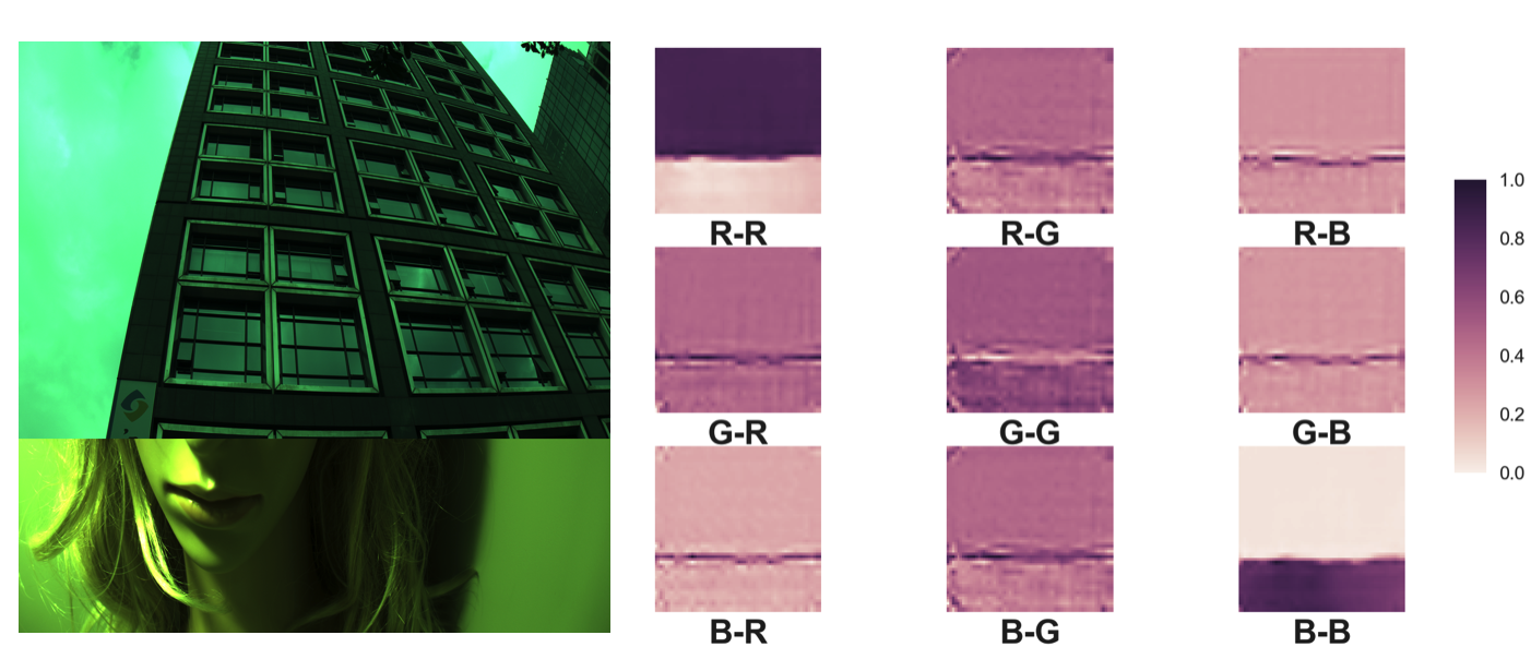
We visualize the learned kernel in Figure 4. The input image is divide and concatenated by two images under distinct illuminants: Here we demonstrate the learned kernel from architecture 64x64x3 / 1x1x3x3 (see supplement). We denote the filter’s channel used for computing the reference’s channel as -. The success of learning shows the aligned kernels (R-R, G-G, B-B) have larger values than the others in Figure 4. From the visualization, we can see that prediction will have less confidence on the boundaries (Equation 9).
Confidence extraction
Considering AWB in camera image processing pipeline, and are normalized with , instead of computing the uniform confidence based on all channels (Equation 10), we practically calculate the confidence on R and B channel as:
| (13) |
where and denote for the mean of and respectively. Equation 13 indicates we expect the mean of confidence of R and B channel to be large and balanced as well. In order to make the confidence estimation more robust and easier to be combined with other algorithms, we separate confidence into five levels (1-5), which span evenly on the range of confidence on training set. Higher level means higher confidence. i.e. Level 5 is the confidence value is bigger than 0.8 times mean confidence value of all training samples. See supplement for more results.
5 Conclusion and Discussion
In this paper, we present self-adaptive kernel learning for single and multi-illuminant estimation. The proposed global-to-local aggregation framework is able to predict region-based illuminant vector (single or multiple according to the clustering results) using the global information instead of training with image patches. We evaluate the proposed method on open source benchmarks, additionally, a self-made benchmark dataset with 13k images has been created for evaluation. Experiments demonstrate our proposed method outperforms the state-of-the-art methods with the largest relative improvement of 16%.
Typical image processing pipeline involves a lot of components which need to be manually finetuned. The proposed framework can be easily extended to other modules in pipeline processing. e.g. color matrix transformation module (CMT). Different from AWB which aims to render the acquired image as closely as possible under the canonical illuminant, CMT transforms the image data into a standard color space. This transformation is needed because the spectral sensitivity functions of the sensor color channels rarely match the desired output color space. CMT is usually performed by using a linear transformation matrix, which could also use the same framework to learn with in a “white box” manner.
The model does not generalize well among differnt cameras sources. For Gehler dataset, experiments show a significant improvement, though, for NUS-8 dataset (images are captured from eight cameras), it shows less improvement due to the optical divergence of its training images. The future work leaves the model-transfer ability to be improved.
References
- (1) N. Banic and S. Loncaric. Color dog-guiding the global illumination estimation to better accuracy. In VISAPP (1), pages 129–135, 2015.
- (2) N. Banic and S. Loncaric. Unsupervised learning for color constancy. CoRR, abs/1712.00436, 2017.
- (3) K. Barnard. Improvements to gamut mapping colour constancy algorithms. In European conference on computer vision, pages 390–403. Springer, 2000.
- (4) K. Barnard, V. Cardei, and B. Funt. A comparison of computational color constancy algorithms. i: Methodology and experiments with synthesized data. IEEE transactions on Image Processing, 11(9):972–984, 2002.
- (5) J. T. Barron. Convolutional color constancy. In Proceedings of the IEEE International Conference on Computer Vision, pages 379–387, 2015.
- (6) J. T. Barron and Y. Tsai. Fast fourier color constancy. CoRR, abs/1611.07596, 2016.
- (7) S. Battiato, G. M. Farinella, M. Guarnera, D. Ravì, and V. Tomaselli. Instant scene recognition on mobile platform. In European Conference on Computer Vision, pages 655–658. Springer, 2012.
- (8) S. Beigpour, C. Riess, J. Van De Weijer, and E. Angelopoulou. Multi-illuminant estimation with conditional random fields. IEEE Transactions on Image Processing, 23(1):83–96, 2014.
- (9) S. Bianco, C. Cusano, and R. Schettini. Color constancy using cnns. In Proceedings of the IEEE Conference on Computer Vision and Pattern Recognition Workshops, pages 81–89, 2015.
- (10) S. Bianco, C. Cusano, and R. Schettini. Single and multiple illuminant estimation using convolutional neural networks. arXiv preprint arXiv:1508.00998, 2015.
- (11) D. H. Brainard and B. A. Wandell. Analysis of the retinex theory of color vision. JOSA A, 3(10):1651–1661, 1986.
- (12) G. Buchsbaum. A spatial processor model for object colour perception. Journal of the Franklin institute, 310(1):1–26, 1980.
- (13) A. Chakrabarti, K. Hirakawa, and T. Zickler. Color constancy with spatio-spectral statistics. IEEE Transactions on Pattern Analysis and Machine Intelligence, 34(8):1509–1519, 2012.
- (14) D. Cheng, D. K. Prasad, and M. S. Brown. Illuminant estimation for color constancy: why spatial-domain methods work and the role of the color distribution. JOSA A, 31(5):1049–1058, 2014.
- (15) D. Cheng, B. Price, S. Cohen, and M. S. Brown. Effective learning-based illuminant estimation using simple features. In Proceedings of the IEEE Conference on Computer Vision and Pattern Recognition, pages 1000–1008, 2015.
- (16) G. D. Finlayson. Corrected-moment illuminant estimation. In Proceedings of the IEEE International Conference on Computer Vision, pages 1904–1911, 2013.
- (17) G. D. Finlayson and E. Trezzi. Shades of gray and colour constancy. In Color and Imaging Conference, volume 2004, pages 37–41. Society for Imaging Science and Technology, 2004.
- (18) P. V. Gehler, C. Rother, A. Blake, T. Minka, and T. Sharp. Bayesian color constancy revisited. In Computer Vision and Pattern Recognition, 2008. CVPR 2008. IEEE Conference on, pages 1–8. IEEE, 2008.
- (19) A. Gijsenij and T. Gevers. Color constancy using natural image statistics and scene semantics. IEEE Transactions on Pattern Analysis and Machine Intelligence, 33(4):687–698, 2011.
- (20) A. Gijsenij, R. Lu, and T. Gevers. Color constancy for multiple light sources. IEEE Transactions on Image Processing, 21(2):697–707, 2012.
- (21) Y. Hu, B. Wang, and S. Lin. Fc 4: Fully convolutional color constancy with confidence-weighted pooling. In Proceedings of the IEEE Conference on Computer Vision and Pattern Recognition, pages 4085–4094, 2017.
- (22) P. Isola, J.-Y. Zhu, T. Zhou, and A. A. Efros. Image-to-image translation with conditional adversarial networks. arXiv preprint, 2017.
- (23) H. R. V. Joze and M. S. Drew. Exemplar-based color constancy and multiple illumination. IEEE transactions on pattern analysis and machine intelligence, 36(5):860–873, 2014.
- (24) H. R. V. Joze, M. S. Drew, G. D. Finlayson, and P. A. T. Rey. The role of bright pixels in illumination estimation. In Color and Imaging Conference, volume 2012, pages 41–46. Society for Imaging Science and Technology, 2012.
- (25) M. Khalil, J.-P. Li, and N. Mustafa. Biologically inspired color perception. In Wavelet Active Media Technology and Information Processing (ICCWAMTIP), 2015 12th International Computer Conference on, pages 198–201. IEEE, 2015.
- (26) D. P. Kingma and J. Ba. Adam: A method for stochastic optimization. arXiv preprint arXiv:1412.6980, 2014.
- (27) Z. Lou, T. Gevers, N. Hu, M. P. Lucassen, et al. Color constancy by deep learning. In BMVC, pages 76–1, 2015.
- (28) B. Mildenhall, J. T. Barron, J. Chen, D. Sharlet, R. Ng, and R. Carroll. Burst denoising with kernel prediction networks. CoRR, abs/1712.02327, 2017.
- (29) J. A. Nelder and R. Mead. A simplex method for function minimization. The computer journal, 7(4):308–313, 1965.
- (30) C. Riess, E. Eibenberger, and E. Angelopoulou. Illuminant color estimation for real-world mixed-illuminant scenes. In Computer Vision Workshops (ICCV Workshops), 2011 IEEE International Conference on, pages 782–789. IEEE, 2011.
- (31) O. Ronneberger, P. Fischer, and T. Brox. U-net: Convolutional networks for biomedical image segmentation. CoRR, abs/1505.04597, 2015.
- (32) W. Shi, C. C. Loy, and X. Tang. Deep specialized network for illuminant estimation. In European Conference on Computer Vision, pages 371–387. Springer, 2016.
- (33) X. Y. Stella and J. Shi. Multiclass spectral clustering. In null, page 313. IEEE, 2003.
- (34) J. Van De Weijer, T. Gevers, and A. Gijsenij. Edge-based color constancy. IEEE Transactions on image processing, 16(9):2207–2214, 2007.