跳到论文正文
W Papers独立论文阅读器 arXiv:1902.04673 论文正文 计算阅读时间 · 0%
引用这篇论文根据当前论文元数据生成,正式投稿前建议核对。


License: arXiv.org perpetual non-exclusive license
arXiv:1902.04673v1 [stat.ME] 12 Feb 2019

Enhanced Balancing of Bias-Variance Tradeoff in Stochastic Estimation: A Minimax Perspective

Henry Lam    Xinyu Zhang    Xuhui Zhang
Abstract

Biased stochastic estimators, such as finite-differences for noisy gradient estimation, often contain parameters that need to be properly chosen to balance impacts from the bias and the variance. While the optimal order of these parameters in terms of the simulation budget can be readily established, the precise best values depend on model characteristics that are typically unknown in advance. We introduce a framework to construct new classes of estimators, based on judicious combinations of simulation runs on sequences of tuning parameter values, such that the estimators consistently outperform a given tuning parameter choice in the conventional approach, regardless of the unknown model characteristics. We argue the outperformance via what we call the asymptotic minimax risk ratio, obtained by minimizing the worst-case asymptotic ratio between the mean square errors of our estimators and the conventional one, where the worst case is over any possible values of the model unknowns. In particular, when the minimax ratio is less than 1, the calibrated estimator is guaranteed to perform better asymptotically. We identify this minimax ratio for general classes of weighted estimators, and the regimes where this ratio is less than 1. Moreover, we show that the best weighting scheme is characterized by a sum of two components with distinct decay rates. We explain how this arises from bias-variance balancing that combats the adversarial selection of the model constants, which can be analyzed via a tractable reformulation of a non-convex optimization problem.

keywords
bias-variance tradeoff, minimax analysis, stochastic estimation, finite difference, robust optimization
††runningauthor: Lam, Zhang and Zhang††runningtitle: Enhanced Bias-Variance Balancing: A Minimax Perspective††authors: Department of Industrial Engineering and Operations Research, Columbia University, New York, NY 10027, khl2114@columbia.edu Department of Industrial Engineering and Operations Research, Columbia University, New York, NY 10027, zhang.xinyu@columbia.edu School for the Gifted Young, University of Science and Technology of China, zxh1998@mail.ustc.edu.cn ††affiliation: ††affiliation: ††affiliation: ††affiliation: ††affiliation: ††affiliation:

1 Introduction

This paper studies biased stochastic estimators which, in the simplest form, are expressed as follows. To estimate a target quantity of interest θ∈ℝ\theta\in\mathbb{R}, we use Monte Carlo simulation where each simulation run outputs

θ^​(δ)=θ+b⁡(δ)+v⁡(δ)\hat{\theta}(\delta)=\theta+b(\delta)+v(\delta) (1)

Here v⁡(δ)v(\delta) represents the noise of the simulation and satisfies E⁡[v⁡(δ)]=0E[v(\delta)]=0, and b⁡(δ)b(\delta) is the bias given by E​[θ^​(δ)]−θE[\hat{\theta}(\delta)]-\theta. We obtain the final estimate by averaging nn independent runs produced by (1):

1n​∑j=1nθ^j​(δ)\frac{1}{n}\sum_{j=1}^{n}\hat{\theta}_{j}(\delta) (2)

where θ^j​(⋅)\hat{\theta}_{j}(\cdot) denotes an independent run.

The simulation runs in (1) are specified by a parameter δ\delta that typically impacts the bias and the variance in an antagonistic fashion. A common example is finite-difference schemes for black-box or zeroth-order noisy gradient estimation, in which δ\delta is the perturbation size for the function input of interest. As δ\delta increases, bias increases while variance decreases (and vice versa). To minimize the mean square error (MSE), the best choice of δ\delta, in terms of the simulation budget, balances the magnitudes of the two error sources. In central finite-difference for instance, this optimal δ\delta turns out to be of order n−1/6n^{-1/6}, whereas in forward or backward finite-difference it is of order n−1/4n^{-1/4} (e.g., Glasserman 2013 Chapter 7; Asmussen and Glynn 2007 Chapter 7; Fu 2006; L’Ecuyer 1991).

While the above tradeoff and the optimal order of δ\delta in nn is well understood in the literature, the precise best choice of δ\delta depends on other, typically unknown, model characteristics (i.e., the “constants” inside b⁡(δ)b(\delta) and v⁡(δ)v(\delta)). For example, choosing δ=dn−1/6\delta=dn^{-1/6} in a central finite-difference, and considering only the first-order error term, the best choice of dd depends on third-order derivative information and the variance of the noise that are typically unavailable in advance.

Our goal in this paper is to develop a framework that enhances the standard estimator (2) regarding the choice of δ\delta subject to the ambiguity of the model characteristics. A key idea we will undertake is to consider estimators beyond the form of naive sample average, in a way that reduces the impact of this uncertainty. Under this framework, we derive new estimators that consistently improve (2) at a given choice of δ\delta, regardless of these unknowns. This improvement is in terms of the asymptotic MSE as the simulation budget increases. More specifically, we consider the asymptotic ratio between the MSEs of any proposed estimator and (2):

R=lim supn→∞MSE of a proposed estimatorMSE of the conventional estimator (2)R=\limsup_{n\to\infty}\frac{\text{MSE of a proposed estimator}}{\text{MSE of the conventional estimator \eqref{simple average}}} (3)

The proposed estimator can be parametrized by possibly many tuning parameters. The asymptotic ratio RR thus contains these parameters, the unknown model characteristics, and the δ\delta in (2). Regarding (2) and its δ\delta as a “baseline”, we calibrate the tuning parameters in the proposed estimator to minimize the worst-case asymptotic MSE ratio, where the worst case is over all possible model characteristics and choices of δ\delta. On a high level, this can be expressed as

R∗=mincalibrationstrategy⁡maxmodelcharacteristics,δ​RR^{*}=\min_{\begin{subarray}{c}\text{calibration}\\ \text{strategy}\end{subarray}}\max_{\begin{subarray}{c}\text{model}\\ \text{characteristics}\end{subarray},\delta}R (4)

This minimized worst-case ratio R∗R^{*} provides a performance guarantee on our calibrated proposed estimator relative to (2) – The MSE of our estimator is asymptotically at most R∗R^{*} of (2) at the chosen δ\delta, independent of any possible model specifications. In particular, if R∗<1R^{*}<1, our estimator is guaranteed to strictly improve over (2). For convenience, we call R∗R^{*} the asymptotic minimax risk ratio (AMRR).

As our main contributions, we systematically identify the AMRR R∗R^{*}, achieve R∗<1R^{*}<1, and construct a scheme that consistently outperforms the conventional choice (2), over the class of weighted estimator in the form

∑j=1nwj​θ^j​(δj)\sum_{j=1}^{n}w_{j}\hat{\theta}_{j}(\delta_{j}) (5)

where δj,j=1,…,n\delta_{j},j=1,\ldots,n is a suitable sequence of tuning parameters, and wj,j=1,…,nw_{j},j=1,\ldots,n is any weighting sequence. When wiw_{i}’s are the uniform weights, (5) is precisely the “recursive estimator” introduced in Glynn and Whitt 1992. This latter estimator selects δj\delta_{j} as if, roughly speaking, the current simulation run jj is the last one in the budget. In other words, given that δ=Θ⁡(n−α)\delta=\Theta(n^{-\alpha}) achieves the optimal MSE order for (2), it selects δj=Θ⁡(j−α)\delta_{j}=\Theta(j^{-\alpha}), and it can be shown to exhibit the same optimal MSE order (the term “recursive” refers to the fact that it can be obtained by iteratively reweighting existing estimates and new runs that depend only on the current run index). This construction can be generalized to stochastic approximation (SA) type recursions (e.g., Duplay et al. 2018), and their averaging version (as in Polyak and Juditsky 1992). Our main results show that, in general, the optimal weighting scheme to obtain R∗R^{*} is in the form

wj=λ1jβ1+λ2jβ2w_{j}=\frac{\lambda_{1}}{j^{\beta_{1}}}+\frac{\lambda_{2}}{j^{\beta_{2}}} (6)

where β1,β2>0\beta_{1},\beta_{2}>0 are two distinct decay rates. The two coefficients λ1,λ2\lambda_{1},\lambda_{2} depends on the budget nn, in a way that none of the two terms in (6) is asymptotically negligible when used in the weighted estimator. This weighting scheme, and an associated transformation from δ\delta to {δj}j\{\delta_{j}\}_{j}, give rise to an explicitly identifiable R∗R^{*} that decreases with an “inflation” factor imposed on the δ\delta-transformation. This reveals that, for instance, in the central finite-difference scheme, R∗R^{*} is 0.670.67 when the multiplicative constants in δ\delta and {δj}j\{\delta_{j}\}_{j} are the same. Since R∗<1R^{*}<1, the weighted estimator using (6) always outperforms (2) in terms of asymptotic MSE, independent of the unknown constants in b⁡(δ)b(\delta) and v⁡(δ)v(\delta). In contrast, the corresponding R∗R^{*} is 1.081.08 when the weights are obtained via standard SA recursion, either with or without averaging, indicating that such a restriction on the weighting sequence could lead to subpar performance in the MSE.

Our main analyses build on the insight that, to maintain a low worst-case risk ratio, one typically must calibrate the proposed estimator such that it maintains the relative magnitudes of bias and variance in a similar manner as the conventional scheme (2). We will show that any distortion away from such a balancing allows an “adversary” to enlarge the risk ratio, thus leading to suboptimal outcomes. This balancing requirement generally leads to a non-convex constrained optimization problem which, upon a reformulation, reveals a tractable structure and solution to the minimax problem in (4).

The remainder of the paper is as follows. Section 2 first reviews some related works. Section 3 describes the problem settings and reviews some established results on biased estimation. Section 4 presents our minimax framework and investigation on a special class of estimators. Section 5 presents our main results and explains their implications on general weighted estimators and AMRR. Section 6 discusses how our results carry to multivariate settings. Section 7 reports our numerical experiments. Section 8 concludes the paper. All proofs are in the Appendix.

2 Related Literature

Our study is related to several lines of work. The minimax formulation that we use to analyze and construct estimators resembles robust optimization (e.g., Ben-Tal et al. 2009, Bertsimas et al. 2011, Ben-Tal and Nemirovski 2002) and robust control (e.g., Zhou and Doyle 1998) that advocates decision-making against the worst-case scenario. Such ideas also have roots in game theory (Cesa-Bianchi and Lugosi 2006). Related notions have also been used in online optimization, in which decision is made at each step under a noisily observed dynamical process (e.g., Flaxman et al. 2005, Shalev-Shwartz et al. 2012, Hazan et al. 2016). The performance in this literature is often measured by the regret that indicates the suboptimality of a decision relative to the best decision assuming complete information (see, e.g., Besbes and Zeevi 2009, Besbes and Zeevi 2011 for applications in revenue management). Instead of using an “oracle” best as the benchmark in our minimax formulation, we use the sample average as our benchmark, and focus on improving this conventional estimator by analyzing the risk ratio. In this regard, we note that a ratio formulation and a non-oracle-best benchmark has been used in Agrawal et al. 2012, but in a different context in quantifying the impact of correlation in mean estimation, and their benchmark is an independent distribution with the worst-case being evaluated over a class of dependent models. Ratios between MSEs also appear in Pasupathy 2010 in studying the tradeoff between error tolerance and sample size in so-called retrospective approximation, which is a technique for solving stochastic root-finding or optimization problems via imposing a sequence of sample average approximation problems.

A main application of our work is finite-difference stochastic gradient estimation (e.g., Glasserman 2013 Chapter 7; Asmussen and Glynn 2007 Chapter 7; Fu 2006; L’Ecuyer 1991), typically used when there is only a noisy simulation oracle to evaluate the function value or model output. Variants of the finite-difference method include the central, forward and backward finite-differences, with different perturbation directions and orders of bias (Zazanis and Suri 1993, Fox and Glynn 1989). In contrast to finite-differences are unbiased derivative estimators, which include the infinitesimal perturbation analysis or pathwise differentiation (Ho et al. 1983, Heidelberger et al. 1988), the likelihood ratio or the score function method (Glynn 1990, Rubinstein 1986, Reiman and Weiss 1989), measure-valued or weak differentiation (Heidergott and Vázquez-Abad 2008, Heidergott et al. 2010), and other variants such as the push-out method (Rubinstein 1992, L’Ecuyer 1990), conditional and smoothed perturbation analysis (Gong and Ho 1987, Hong 2009, Fu and Hu 1992, Glasserman and Gong 1990, Fu et al. 2009) and the generalized likelihood ratio method (Peng et al. 2018). In multivariate settings, Spall 1992, Spall 1997 study simultaneous perturbation to estimate gradients used in SA, by randomly generating a perturbation direction vector and properly weighting with the perturbation sizes to control estimation bias. Nesterov and Spokoiny 2017 proposes Gaussian smoothing with a different adjustment and investigates finite-sample behaviors in related optimization. Flaxman et al. 2005 suggests uniform sampling. Our framework can be applied to these procedures, as will be discussed in Section 6.

The main skeleton of our proposed estimators uses a sequentialized choice of the tuning parameter, which appears in Glynn and Whitt 1992 in their discussion of subcanonical estimators. A special case of our scheme, discussed in Section 4, resembles the idea of SA in stochastic optimization and root-finding that iteratively updates noisy estimates (Kushner and Yin 2003, Borkar 2009, Pasupathy and Kim 2011, Nemirovski et al. 2009, Polyak and Juditsky 1992, Ruppert 1988). Our analyses there utilize the classical asymptotic techniques in Fabian 1968 and Chung 1954, and also Polyak and Juditsky 1992 in the averaging case.

We close this section by briefly comparing our work to multi-level Monte Carlo (Giles 2008). This approach aims to reduce variance in simulation in the presence of a parameter selection like δ\delta, by stratifying the simulation budget into different δ\delta values. Of particular relevance is the randomized level selection (Rhee and Glynn 2015, Blanchet and Glynn 2015, Rychlik 1990, McLeish 2010) that can turn biased estimators in the form of (1) into unbiased estimators with canonical square-root convergence. This approach has been applied in the simulation of stochastic differential equations and nonlinear functions of expectations, and requires a proper coupling between simulation runs at consecutive levels to control the simulation effort. In investigating (1), we do not assume any problem structure that allows such coupling, and our performance is benchmarked against the conventional (biased) sample-average scheme.

3 Background and Problem Setting

We elaborate our problem and notations in the introduction. We are interested in estimating θ∈ℝ\theta\in\mathbb{R}. Given a tuning parameter δ∈ℝ+\delta\in\mathbb{R}_{+}, we run Monte Carlo simulation where each run outputs

θ^​(δ)=θ+b⁡(δ)+v⁡(δ)\hat{\theta}(\delta)=\theta+b(\delta)+v(\delta) (7)

with b⁡(δ)=B​δq1+o⁡(δq1)b(\delta)=B\delta^{q_{1}}+o(\delta^{q_{1}}) as δ→0\delta\to 0, v⁡(δ)=ε⁡(δ)δq2v(\delta)=\frac{\varepsilon(\delta)}{\delta^{q_{2}}}, and q1,q2>0q_{1},q_{2}>0. We assume that: {assumption} We have

  1. 1.

    B∈ℝB\in\mathbb{R} is a non-zero constant.

  2. 2.

    ε⁡(δ)∈ℝ\varepsilon(\delta)\in\mathbb{R} is a random variable such that E​ε​(δ)=0E\varepsilon(\delta)=0 and σ2​(δ)=V​a​r​(ε⁡(δ))→σ2>0\sigma^{2}(\delta)=Var(\varepsilon(\delta))\to\sigma^{2}>0 as δ→0\delta\to 0.

The above assumptions dictate that the order of the bias b⁡(δ)b(\delta) is δq1\delta^{q_{1}}, while the order of the variance is δ−2​q2\delta^{-2q_{2}}. The former is ensured by the first assumption and the latter by the second one.

As an example, in estimating the derivative of a function f⁡(x)f(x) with unbiased noisy function evaluation, the central finite-difference (CFD) scheme elicits the output

f^​(x+δ)−f^​(x−δ)2​δ\frac{\hat{f}(x+\delta)-\hat{f}(x-\delta)}{2\delta}

where f^​(⋅)\hat{f}(\cdot) is an unbiased evaluation of f⁡(⋅)f(\cdot), and δ>0\delta>0 is the perturbation size. Given that ff is thrice continuously differentiable with non-zero f′′′​(x)f^{\prime\prime\prime}(x), the bias term has order q1=2q_{1}=2. Typically, the order of the variance is q2=1q_{2}=1. Suppose we do not apply common random numbers (CRN) in generating f^​(x+δ)\hat{f}(x+\delta) and f^​(x−δ)\hat{f}(x-\delta), and that V​a​r​(f^​(x±δ))→V​a​r​(f^​(x))Var(\hat{f}(x\pm\delta))\to Var(\hat{f}(x)) as δ→0\delta\to 0, then σ2=V​a​r​(f^​(x))/2\sigma^{2}=Var(\hat{f}(x))/2. Suppose we are able to apply CRN so that C​o​v​(f^​(x+δ),f^​(x−δ))→ρCov(\hat{f}(x+\delta),\hat{f}(x-\delta))\to\rho as δ→0\delta\to 0 (i.e., we cannot fully eliminate the first-order variance as δ\delta shrinks), then we have σ2=(V​a​r​(f^​(x))−ρ)/2\sigma^{2}=(Var(\hat{f}(x))-\rho)/2.

Similarly, the forward finite-difference (FFD) scheme elicits the output

f^​(x+δ)−f^​(x)δ\frac{\hat{f}(x+\delta)-\hat{f}(x)}{\delta}

Given that ff is twice continuously differentiable with non-zero f′′​(x)f^{\prime\prime}(x), the bias term has order q1=1q_{1}=1. Analogous conditions on the noise as above guarantees that q2=1q_{2}=1. The same discussion holds for the backward finite-difference (BFD) scheme.

Given the capability to output independent runs of (7), say θ^j​(δ)\hat{\theta}_{j}(\delta), the conventional approach to obtain an estimate of θ\theta is to take their sample average. Denote this as θ¯n=(1/n)​∑j=1nθ^j​(δ)\bar{\theta}_{n}=(1/n)\sum_{j=1}^{n}\hat{\theta}_{j}(\delta). The MSE of θ¯n\bar{\theta}_{n}, denoted MSE0=E​(θ¯n−θ)2\text{MSE}_{0}=E(\bar{\theta}_{n}-\theta)^{2}, can be expressed as

MSE0=bias2+variance=B2​δ2​q1+σ2n​δ2​q2+higher-order terms\text{MSE}_{0}=\text{bias}^{2}+\text{variance}=B^{2}\delta^{2q_{1}}+\frac{\sigma^{2}}{n\delta^{2q_{2}}}+\text{higher-order terms} (8)

Considering the first order term, the bias increases with δ\delta and the variance decreases with δ\delta. Minimizing the MSE requires balancing these two errors to the same order, namely by choosing δ=Θ⁡(n−α)\delta=\Theta(n^{-\alpha}) where α=1/(2​(q1+q2))\alpha=1/(2(q_{1}+q_{2})), which solves the equation −2​α​q1=−1+2​α​q2-2\alpha q_{1}=-1+2\alpha q_{2}. This leads to an optimal MSE order n−q1/(q1+q2)n^{-q_{1}/(q_{1}+q_{2})}. For example, in CFD and under the conditions we discussed above, we have δ=Θ(n−1/6)\delta=\Theta(n^{-1/6}), leading to an optimal MSE order n−2/3n^{-2/3}; in FFD or BFD we have δ=Θ(n−1/4)\delta=\Theta(n^{-1/4}), leading to an optimal MSE order n−1/2n^{-1/2}.

In order to fully optimize the first-order MSE, including the coefficient, one needs to choose

δ=(σ2​q2B2​q1)1/(2​(q1+q2))​1n1/(2​(q1+q2))\delta=\left(\frac{\sigma^{2}q_{2}}{B^{2}q_{1}}\right)^{1/(2(q_{1}+q_{2}))}\frac{1}{n^{1/(2(q_{1}+q_{2}))}}

(e.g., by applying the first-order optimality condition on the leading terms in (8)). This gives an optimal first-order MSE

B2​q2/(q1+q2)​σ2​q1/(q1+q2)​((q2q1)q1/(q1+q2)+(q1q2)q2/(q1+q2))​1nq1/(q1+q2)B^{2q_{2}/(q_{1}+q_{2})}\sigma^{2q_{1}/(q_{1}+q_{2})}\left(\left(\frac{q_{2}}{q_{1}}\right)^{q_{1}/(q_{1}+q_{2})}+\left(\frac{q_{1}}{q_{2}}\right)^{q_{2}/(q_{1}+q_{2})}\right)\frac{1}{n^{q_{1}/(q_{1}+q_{2})}} (9)

The above choice of δ\delta depends on the “constants” in the bias and variance terms, namely BB and σ2\sigma^{2}. While q1q_{1} and q2q_{2} are often obtainable, constants like BB and σ2\sigma^{2} are unknown a priori and can affect the performance of the simulation estimator, despite choosing an optimal order on nn in δ\delta using the knowledge of q1q_{1} and q2q_{2}. Suppose we choose δ=d/nα\delta=d/n^{\alpha} for some d>0d>0, where α=1/(2​(q1+q2))\alpha=1/(2(q_{1}+q_{2})) is optimally chosen. Then the first-order MSE is

(B2​d2​q1+σ2d2​q2)​1nq1/(q1+q2)\left(B^{2}d^{2q_{1}}+\frac{\sigma^{2}}{d^{2q_{2}}}\right)\frac{1}{n^{q_{1}/(q_{1}+q_{2})}} (10)

which can be arbitrarily suboptimal relative to the best coefficient in (9). Our goal in this paper is to improve on this suboptimality, by considering estimators beyond the conventional sample average that consistently outperforms the constant showing up in (10).

The following theorem, which follow straightforwardly from Fox and Glynn 1989, summarizes the above discussion on the optimal order of the MSE:

Theorem 3.1

Under Assumption 3, suppose that limn→∞δ​nα=d>0\lim_{n\to\infty}\delta n^{\alpha}=d>0, the sample-average-based estimator θ¯n\bar{\theta}_{n} exhibits the asymptotic MSE

E​(θ¯n−θ)2=d2​q1​B2​n−2​α​q1+σ2d2​q2​n2​α​q2−1+o⁡(n−2​α​q1+n2​α​q2−1)​ as ​n→∞E(\bar{\theta}_{n}-\theta)^{2}=d^{2q_{1}}B^{2}n^{-2\alpha q_{1}}+\frac{\sigma^{2}}{d^{2q_{2}}}n^{2\alpha q_{2}-1}+o(n^{-2\alpha q_{1}}+n^{2\alpha q_{2}-1})\textrm{ as }n\to\infty

Choosing α=1/(2​(q1+q2))\alpha=1/(2(q_{1}+q_{2})) achieves the optimal MSE order, and the asymptotic MSE is

E(θ¯n−θ)2=(d2​q1B2+σ2d2​q2)n−q1/(q1+q2)+o(n−q1/(q1+q2)) as n→∞E(\bar{\theta}_{n}-\theta)^{2}=\big(d^{2q_{1}}B^{2}+\frac{\sigma^{2}}{d^{2q_{2}}}\big)n^{-q_{1}/(q_{1}+q_{2})}+o(n^{-q_{1}/(q_{1}+q_{2})})\text{ as }n\to\infty

Lastly, we mention that, in practice, there are other considerations in obtaining good estimators, such as issues regarding the finiteness of the sample that can affect the accuracy of the asymptotic results. These considerations are beyond the scope of this work, which focuses mainly on a theoretical framework on improving the asymptotic constant.

4 A Minimax Comparison Framework

We introduce a framework to assess, and calibrate, estimators beyond the sample-average-based estimator θ¯n\bar{\theta}_{n}. This framework compares the asymptotic MSEs using θ¯n\bar{\theta}_{n} as a baseline based on a minimax argument. Section 4.1 presents this framework, and Section 4.2 provides an initial study on a special type of estimators.

4.1 Asymptotic Risk Ratio

Consider an estimator θ^n\hat{\theta}_{n} for θ\theta using nn simulation runs in the form (7), where the tuning parameter δ\delta in each run can be arbitrarily chosen. Our goal is to calibrate θ^n\hat{\theta}_{n} that performs well, or outperforms, θ¯n\bar{\theta}_{n} in the first-order coefficient of the MSE, presuming that both θ^n\hat{\theta}_{n} and θ¯n\bar{\theta}_{n} have the optimal order of errors. Let MSE1\text{MSE}_{1} denote the MSE of θ^n\hat{\theta}_{n} for convenience.

The estimator θ^n\hat{\theta}_{n} can depend on other tuning parameters in addition to the δ\delta in each run. We denote the collection of all the parameters that θ^n\hat{\theta}_{n} involves as ν\nu, so that θ^n=θ^n​(ν)\hat{\theta}_{n}=\hat{\theta}_{n}(\nu). Correspondingly, MSE1\text{MSE}_{1} also depends on ν\nu.

We suppose knowledge on the order of the bias and noise, namely q1q_{1} and q2q_{2} in (7). However, we do not know the constants BB and σ2\sigma^{2}. To make the discussion more precise, for fixed q1,q2>0q_{1},q_{2}>0, we denote the class of simulation outputs

Θ\displaystyle\Theta =\displaystyle= {θ^(⋅):θ^(δ)=θ+b(δ)+v(δ) such that\displaystyle\big\{\hat{\theta}(\cdot):\hat{\theta}(\delta)=\theta+b(\delta)+v(\delta)\text{\ such that\ } (11)
b⁡(δ)=B​δq1+o⁡(δq1)​ and ​v​(δ)=ε⁡(δ)δq2​ where ​V​a​r​(ϵ⁡(δ))→σ2, as ​δ→0,\displaystyle{}b(\delta)=B\delta^{q_{1}}+o(\delta^{q_{1}})\text{\ and\ }v(\delta)=\frac{\varepsilon(\delta)}{\delta^{q_{2}}}\text{\ where\ }Var(\epsilon(\delta))\to\sigma^{2},\text{\ as\ }\delta\to 0,{}
for arbitrary non-zero B and positive σ2}\displaystyle{}\text{\ for arbitrary non-zero $B$ and positive $\sigma^{2}$}\big\}

In other words, Θ\Theta is the set of outputs with bias of order δq1\delta^{q_{1}} and noise of order δ−q2\delta^{-q_{2}}, with arbitrary constants BB, σ2\sigma^{2}, and the higher-order error terms.

The MSE of θ¯n\bar{\theta}_{n}, MSE0\text{MSE}_{0}, depends on θ^​(⋅)\hat{\theta}(\cdot) evaluated at chosen δ\delta. To highlight this dependence, we write MSE0=MSE0​(θ^​(⋅),δ)\text{MSE}_{0}=\text{MSE}_{0}(\hat{\theta}(\cdot),\delta). Similarly, MSE1\text{MSE}_{1} depends on θ^​(⋅)\hat{\theta}(\cdot) and ν\nu, so that MSE1=MSE1​(θ^​(⋅),ν)\text{MSE}_{1}=\text{MSE}_{1}(\hat{\theta}(\cdot),\nu). We consider the asymptotic risk ratio

R⁡(θ^​(⋅),ν,δ)=lim supn→∞MSE1​(θ^​(⋅),ν)MSE0​(θ^​(⋅),δ)R(\hat{\theta}(\cdot),\nu,\delta)=\limsup_{n\to\infty}\frac{\text{MSE}_{1}(\hat{\theta}(\cdot),\nu)}{\text{MSE}_{0}(\hat{\theta}(\cdot),\delta)} (12)

that measures the performance of θ^n\hat{\theta}_{n} relative to θ¯n\bar{\theta}_{n} as a baseline. Since we only know θ^​(⋅)\hat{\theta}(\cdot) is in Θ\Theta but not its exact forms (i.e., the constants), we consider the worst-case scenario of RR, and search for the best parameters in θ^n\hat{\theta}_{n} that minimize this worst-case risk. Namely, we aim to solve

minν⁡maxθ^​(⋅)∈Θ⁡R⁡(θ^​(⋅),ν,δ)\min_{\nu}\max_{\hat{\theta}(\cdot)\in\Theta}R(\hat{\theta}(\cdot),\nu,\delta) (13)

Note that (13), and the best choice of ν\nu, depend on the δ\delta used in θ¯n\bar{\theta}_{n}. We now take a further viewpoint that an arbitrary user may select any δ\delta, and we look for a strategy to calibrate θ^n\hat{\theta}_{n} that is guaranteed to perform well no matter how δ\delta is chosen. To write this more explicitly, we let ν=ν⁡(δ)\nu=\nu(\delta) be dependent on δ\delta, and we search for the best collection of parameters that is potentially a function ν⁡(⋅)\nu(\cdot) on δ\delta:

R∗=minν⁡(⋅)∈Λ⁡maxθ^​(⋅)∈Θ,δ∈ℝ⁡R⁡(θ^​(⋅),ν⁡(⋅),δ)R^{*}=\min_{\nu(\cdot)\in\Lambda}\max_{\hat{\theta}(\cdot)\in\Theta,\delta\in\mathbb{R}}R(\hat{\theta}(\cdot),\nu(\cdot),\delta) (14)

where Λ\Lambda denotes the set of admissible functions ν⁡(⋅)\nu(\cdot). This set Λ\Lambda depends on the class of estimators θ^n\hat{\theta}_{n} we use, which will be described in detail. Moreover, as we will see, (13) and (14) are closely related; in fact, under the settings we consider, solving either of them simultaneously solves another. In the following, we will focus on (14) and discuss the immediate implications on (13) where appropriate. We shall call R∗R^{*} the asymptotic minimax risk ratio (AMRR).

4.2 An Initial Example: Recursive Estimators

For convenience, let us from now on set δ=d​(n+n0)−α\delta=d(n+n_{0})^{-\alpha} as the tuning parameter in the sample-average-based estimator θ¯n\bar{\theta}_{n}, where α=1/(2​(q1+q2))\alpha=1/(2(q_{1}+q_{2})) so that it achieves the optimal MSE order. The number n0n_{0} can be any fixed integer to prevent δ\delta from being too big at the early stage, and does not affect our asymptotic analyses.

To construct our proposed estimator θ^n\hat{\theta}_{n}, we will first use the idea of the recursive estimator studied in Section 5 of Glynn and Whitt 1992. At run jj, we simulate θ^j​(δj)\hat{\theta}_{j}(\delta_{j}), where δj=d~​(j+n0)−α\delta_{j}=\tilde{d}(j+n_{0})^{-\alpha} for some constant d~\tilde{d}, and α\alpha is the same as in θ¯n\bar{\theta}_{n}, i.e., the parameter is chosen as if the current simulation run is the last one in the budget if a conventional sample-average-based estimator is used. The estimator in Glynn and Whitt 1992 uses the average of θ^j​(δj)\hat{\theta}_{j}(\delta_{j}), namely (1/n)​∑j=1nθ^j​(δj)(1/n)\sum_{j=1}^{n}\hat{\theta}_{j}(\delta_{j}). As shown in Glynn and Whitt 1992, this estimator exhibits the optimal MSE order like θ¯n\bar{\theta}_{n}. Moreover, as they have also noted, this estimator admits a recursive representation θ^n=(1−1/n)​θ^n−1+(1/n)​θ^n​(δn)\hat{\theta}_{n}=(1-1/n)\hat{\theta}_{n-1}+(1/n)\hat{\theta}_{n}(\delta_{n}), where each update depends only on the parameter indexed by the current run number, rather than the budget. Thus, the optimal MSE order is achieved in an “online” fashion as nn increases, independent of the final budget.

The initial class of estimators that we will consider is a generalization of Glynn and Whitt 1992. Specifically, we consider estimators defined via the recursion

θ^nr​e​c=(1−γn)​θ^n−1r​e​c+γn​θ^n​(δn)\hat{\theta}_{n}^{rec}=\left(1-\gamma_{n}\right)\hat{\theta}_{n-1}^{rec}+\gamma_{n}\hat{\theta}_{n}(\delta_{n}) (15)

where δn=d~​(n+n0)−α\delta_{n}=\tilde{d}(n+n_{0})^{-\alpha} is defined as before and α>0\alpha>0, and γn\gamma_{n} is in the form c​(n+n0)−βc(n+n_{0})^{-\beta} for some c>0c>0 and β>0\beta>0. θ^0r​e​c\hat{\theta}_{0}^{rec} can be arbitrary. Moreover, we also consider averaging θ^nr​e​c\hat{\theta}_{n}^{rec} in the form

θ^na​v​g=1n​∑j=1nθ^jr​e​c\hat{\theta}_{n}^{avg}=\frac{1}{n}\sum_{j=1}^{n}\hat{\theta}_{j}^{rec} (16)

which resembles the standard Polyak-Ruppert averaging in SA (Polyak and Juditsky 1992).

Our first result is that, in terms of the AMRR, the class of estimators θ^nr​e​c\hat{\theta}_{n}^{rec} and θ^na​v​g\hat{\theta}_{n}^{avg} are quite restrictive and cannot bring in much improvement over θ¯n\bar{\theta}_{n}. To elicit this result, we begin with some consistency properties of θ^nr​e​c\hat{\theta}_{n}^{rec}:

Proposition 4.1

Under Assumption 3, we have:

  1. 1.

    If β≤1\beta\leq 1 and α<β/(2​q2)\alpha<\beta/(2q_{2}), the estimator θ^nr​e​c\hat{\theta}_{n}^{rec} is L2L_{2}-consistent for θ\theta, i.e.,

    limn→∞E​(θ^nr​e​c−θ)2=0\lim_{n\to\infty}E(\hat{\theta}_{n}^{rec}-\theta)^{2}=0
  2. 2.

    If β≤1\beta\leq 1 and α≥β/(2​q2)\alpha\geq\beta/(2q_{2}), or if β>1\beta>1, the error of θ^nr​e​c\hat{\theta}_{n}^{rec} in estimating θ\theta is bounded away from zero in L2L_{2}-norm as n→∞n\to\infty, i.e.,

    lim infn→∞E​(θ^nr​e​c−θ)2>0\liminf_{n\to\infty}E(\hat{\theta}_{n}^{rec}-\theta)^{2}>0

Proposition 4.1 shows that θ^nr​e​c\hat{\theta}_{n}^{rec} estimates θ\theta sensibly only when β≤1\beta\leq 1 and α<β/(2​q2)\alpha<\beta/(2q_{2}). We thus focus on this case subsequently. The following describes the convergence rate:

Theorem 4.2

Under Assumption 3, the MSE of θ^nr​e​c\hat{\theta}_{n}^{rec} in estimating θ\theta behaves as follows:

  1. 1.

    For β<1\beta<1 and α<β/(2​q2)\alpha<\beta/(2q_{2}),

    E​(θ^nr​e​c−θ)2=d2​q1​B2​n−2​q1​α+c​σ22​d2​q2​n2​q2​α−β+o⁡(n−2​q1​α+n2​q2​α−β)​ as ​n→∞E(\hat{\theta}_{n}^{rec}-\theta)^{2}=d^{2q_{1}}B^{2}n^{-2q_{1}\alpha}+\frac{c\sigma^{2}}{2d^{2q_{2}}}n^{2q_{2}\alpha-\beta}+o(n^{-2q_{1}\alpha}+n^{2q_{2}\alpha-\beta})\text{ as }n\to\infty
  2. 2.

    For β=1\beta=1, α=1/(2​(q1+q2))\alpha=1/(2(q_{1}+q_{2})) and c>q1/(2​(q1+q2))c>q_{1}/(2(q_{1}+q_{2})),

    E(θ^nr​e​c−θ)2=((c​dq1c−q1/(2​(q1+q2)))2B2+c2​σ2(2​c−q1/(q1+q2))​d2​q2)n−q1/(q1+q2)+o(n−q1/(q1+q2)) as n→∞E(\hat{\theta}_{n}^{rec}-\theta)^{2}=\left(\big(\frac{cd^{q_{1}}}{c-q_{1}/(2(q_{1}+q_{2}))}\big)^{2}B^{2}+\frac{c^{2}\sigma^{2}}{(2c-q_{1}/(q_{1}+q_{2}))d^{2q_{2}}}\right)n^{-q_{1}/(q_{1}+q_{2})}+o(n^{-q_{1}/(q_{1}+q_{2})})\text{ as }n\to\infty
  3. 3.

    For β=1\beta=1, α=1/(2​(q1+q2))\alpha=1/(2(q_{1}+q_{2})) and c≤q1/(2​(q1+q2))c\leq q_{1}/(2(q_{1}+q_{2})), or for β=1\beta=1 and α≠1/(2​(q1+q2))\alpha\neq 1/(2(q_{1}+q_{2})),

    lim supn→∞nq1/(q1+q2)​E​(θ^nr​e​c−θ)2=∞\limsup_{n\to\infty}n^{q_{1}/(q_{1}+q_{2})}E(\hat{\theta}_{n}^{rec}-\theta)^{2}=\infty

The proofs of the above results, which are detailed in Appendix B, utilize the classical asymptotic techniques for recursive sequences in Fabian 1968 and a slight modification of Chung’s lemma (i.e., Lemma B.1 in Appendix B).

We now look at the AMRR for θ^nr​e​c\hat{\theta}_{n}^{rec}. First, Theorem 4.2 shows that the choice β=1,α=1/(2​(q1+q2))\beta=1,\alpha=1/(2(q_{1}+q_{2})) is the unique choice that gives rise to the optimal MSE order n−q1/(q1+q2)n^{-q_{1}/(q_{1}+q_{2})}. Moreover, given this choice of α\alpha, we need c>q1/(2​(q1+q2))c>q_{1}/(2(q_{1}+q_{2})), in addition to β=1\beta=1. We will focus on these configurations for θ^nr​e​c\hat{\theta}_{n}^{rec} that achieve the same MSE order as the conventional estimator θ¯n\bar{\theta}_{n} with the same α\alpha.

Suppose we set d~=d\tilde{d}=d, but allow the free selection of cc within the range that gives rise to the optimal MSE order. We thus can write θ^nr​e​c=θ^nr​e​c​(d,c)\hat{\theta}_{n}^{rec}=\hat{\theta}_{n}^{rec}(d,c), defined via (15) with γn=c​(n+n0)−1\gamma_{n}=c(n+n_{0})^{-1} where c>q1/(2​(q1+q2))c>q_{1}/(2(q_{1}+q_{2})). The integer n0n_{0} does not affect any asymptotic and can be taken as any given value. The following characterizes the AMRR and the configuration that attains it:

Theorem 4.3

Under Assumption 3, let MSE1r​e​c​(θ^​(⋅),d,c)\text{MSE}_{1}^{rec}(\hat{\theta}(\cdot),d,c) be the MSE of θ^nr​e​c​(d,c)\hat{\theta}_{n}^{rec}(d,c), and

Rr​e​c​(θ^​(⋅),d,c)=lim supn→∞MSE1r​e​c​(θ^​(⋅),d,c)MSE0​(θ^​(⋅),d)R^{rec}(\hat{\theta}(\cdot),d,c)=\limsup_{n\to\infty}\frac{\text{MSE}_{1}^{rec}(\hat{\theta}(\cdot),d,c)}{\text{MSE}_{0}(\hat{\theta}(\cdot),d)}

We have

minc>q12​(q1+q2)⁡maxθ^​(⋅)∈Θ,d>0​Rr​e​c​(θ^​(⋅),d,c)=q1216​(q1+q2)2+q12​(q1+q2)+1\min_{c>\frac{q_{1}}{2(q_{1}+q_{2})}}\,\max_{\hat{\theta}(\cdot)\in\Theta,d>0}R^{rec}(\hat{\theta}(\cdot),d,c)=\frac{q_{1}^{2}}{16(q_{1}+q_{2})^{2}}+\frac{q_{1}}{2(q_{1}+q_{2})}+1

which is attained by choosing c=5​q1+4​q22​(q1+q2)c=\frac{5q_{1}+4q_{2}}{2(q_{1}+q_{2})}.

Next, we provide more flexibility in the choice of d~\tilde{d} in θ^nr​e​c​(d~,c)\hat{\theta}_{n}^{rec}(\tilde{d},c). In particular, rather than setting d~=d\tilde{d}=d, we allow d~\tilde{d} to depend on dd in any arbitrary fashion, i.e., d~=g⁡(d)\tilde{d}=g(d) where g⁡(⋅):ℝ+→ℝ+g(\cdot):\mathbb{R}_{+}\to\mathbb{R}_{+} is any function. Let ℱ\mathcal{F} be the space of any functions from ℝ+\mathbb{R}_{+} to ℝ+\mathbb{R}_{+}. We have the following results on the AMRR of this enhanced scheme:

Theorem 4.4

Under Assumption 3, let MSE1r​e​c​(θ^​(⋅),d~,c)\text{MSE}_{1}^{rec}(\hat{\theta}(\cdot),\tilde{d},c) be the MSE of θ^nr​e​c​(d~,c)\hat{\theta}_{n}^{rec}(\tilde{d},c), and

Rr​e​c​(θ^​(⋅),d,d~,c)=lim supn→∞MSE1r​e​c​(θ^​(⋅),d~,c)MSE0​(θ^​(⋅),d)R^{rec}(\hat{\theta}(\cdot),d,\tilde{d},c)=\limsup_{n\to\infty}\frac{\text{MSE}_{1}^{rec}(\hat{\theta}(\cdot),\tilde{d},c)}{\text{MSE}_{0}(\hat{\theta}(\cdot),d)}

We have

ming⁡(⋅)∈ℱ,c>q12​(q1+q2)⁡maxθ^​(⋅)∈Θ,d>0​Rr​e​c​(θ^​(⋅),d,g⁡(d),c)=22​q2q1+q2​(q1+2​q2q1+q2)−q1+2​q2q1+q2\min_{g(\cdot)\in\mathcal{F},c>\frac{q_{1}}{2(q_{1}+q_{2})}}\,\max_{\hat{\theta}(\cdot)\in\Theta,d>0}R^{rec}(\hat{\theta}(\cdot),d,g(d),c)=2^{\frac{2q_{2}}{q_{1}+q_{2}}}(\frac{q_{1}+2q_{2}}{q_{1}+q_{2}})^{-\frac{q_{1}+2q_{2}}{q_{1}+q_{2}}}

which is attained by choosing g⁡(d)=(q1+2​q24​(q1+q2))12​(q1+q2)​dg(d)=(\frac{q_{1}+2q_{2}}{4(q_{1}+q_{2})})^{\frac{1}{2(q_{1}+q_{2})}}d and c=1c=1.

We note that Theorem 4.4 indicates c=1c=1 is optimal in this enhanced scheme, while the optimal d~\tilde{d} is chosen as a constant factor ((q1+2​q2)/(4​(q1+q2)))1/(2​(q1+q2))((q_{1}+2q_{2})/(4(q_{1}+q_{2})))^{1/(2(q_{1}+q_{2}))} of dd.

Next we look at θ^na​v​g\hat{\theta}_{n}^{avg}. It turns out that the AMRR depicted for θ^nr​e​c\hat{\theta}_{n}^{rec} in Theorem 4.4 applies also to θ^na​v​g\hat{\theta}_{n}^{avg}. To this end, we first state the MSE of θ^na​v​g\hat{\theta}_{n}^{avg}:

Theorem 4.5

Under Assumption 3, the MSE of θ^na​v​g\hat{\theta}_{n}^{avg} in estimating θ\theta behaves as follows:

  1. 1.

    For β<1\beta<1 and α≤1/(2​(q1+q2))\alpha\leq 1/(2(q_{1}+q_{2})),

    E​(θ^na​v​g−θ)2=(dq11−q1​α)2​B2​n−2​q1​α+σ2(1+2​q2​α)​d2​q2​n2​q2​α−1+o⁡(n−2​q1​α+n2​q2​α−1)​ as ​n→∞E(\hat{\theta}_{n}^{avg}-\theta)^{2}=\big(\frac{d^{q_{1}}}{1-q_{1}\alpha}\big)^{2}B^{2}n^{-2q_{1}\alpha}+\frac{\sigma^{2}}{(1+2q_{2}\alpha)d^{2q_{2}}}n^{2q_{2}\alpha-1}+o(n^{-2q_{1}\alpha}+n^{2q_{2}\alpha-1})\text{ as }n\to\infty
  2. 2.

    For β<1\beta<1 and α>1/(2​(q1+q2))\alpha>1/(2(q_{1}+q_{2})),

    E​(θ^na​v​g−θ)2=σ2(1+2​q2​α)​d2​q2​n2​q2​α−1+o⁡(n2​q2​α−1)​ as ​n→∞E(\hat{\theta}_{n}^{avg}-\theta)^{2}=\frac{\sigma^{2}}{(1+2q_{2}\alpha)d^{2q_{2}}}n^{2q_{2}\alpha-1}+o(n^{2q_{2}\alpha-1})\text{ as }n\to\infty

Comparing Theorem 4.5 with Theorem 4.2, we see that the first-order MSE of θ^na​v​g\hat{\theta}_{n}^{avg} in the considered regime exactly equals that of θ^nr​e​c\hat{\theta}_{n}^{rec} when c=1c=1 and β=1\beta=1. Like before, α=1/(2​(q1+q2))\alpha=1/(2(q_{1}+q_{2})) is the unique choice that optimizes the MSE order for θ^na​v​g\hat{\theta}_{n}^{avg}. Thus, we will focus on this choice of α\alpha in θ^na​v​g\hat{\theta}_{n}^{avg}. Note that then θ^na​v​g=θ^na​v​g​(d~,c,β)\hat{\theta}_{n}^{avg}=\hat{\theta}_{n}^{avg}(\tilde{d},c,\beta) depends on d~,c,β\tilde{d},c,\beta. This leads us to the following AMRR:

Theorem 4.6

Under Assumption 3, let MSE1a​v​g​(θ^​(⋅),d~,c,β)\text{MSE}_{1}^{avg}(\hat{\theta}(\cdot),\tilde{d},c,\beta) be the MSE of θ^na​v​g=θ^na​v​g​(d~,c,β)\hat{\theta}_{n}^{avg}=\hat{\theta}_{n}^{avg}(\tilde{d},c,\beta). Let

Ra​v​g​(θ^​(⋅),d,d~,c,β)=lim supn→∞MSE1a​v​g​(θ^​(⋅),d~,c,β)MSE0​(θ^​(⋅),d)R^{avg}(\hat{\theta}(\cdot),d,\tilde{d},c,\beta)=\limsup_{n\to\infty}\frac{\text{MSE}_{1}^{avg}(\hat{\theta}(\cdot),\tilde{d},c,\beta)}{\text{MSE}_{0}(\hat{\theta}(\cdot),d)}

We have

ming⁡(⋅)∈ℱ,c>0,0<β<1⁡maxθ^​(⋅)∈Θ,d>0​Ra​v​g​(θ^​(⋅),d,g⁡(d),c,β)=22​q2q1+q2​(q1+2​q2q1+q2)−q1+2​q2q1+q2\min_{g(\cdot)\in\mathcal{F},c>0,0<\beta<1}\,\max_{\hat{\theta}(\cdot)\in\Theta,d>0}R^{avg}(\hat{\theta}(\cdot),d,g(d),c,\beta)=2^{\frac{2q_{2}}{q_{1}+q_{2}}}(\frac{q_{1}+2q_{2}}{q_{1}+q_{2}})^{-\frac{q_{1}+2q_{2}}{q_{1}+q_{2}}}

which is attained by choosing g⁡(d)=(q1+2​q24​(q1+q2))12​(q1+q2)​dg(d)=(\frac{q_{1}+2q_{2}}{4(q_{1}+q_{2})})^{\frac{1}{2(q_{1}+q_{2})}}d, and any c>0c>0 and 0<β<10<\beta<1.

The minimax ratios stated in Theorems 4.3, 4.4 and 4.6 remain the same, in a uniform fashion, when the parameter dd in θ¯n\bar{\theta}_{n} is fixed instead of being chosen by an adversarial user. In other words, the minimax risk ratio of θ^nr​e​c\hat{\theta}_{n}^{rec} or θ^na​v​g\hat{\theta}_{n}^{avg} compared to θ¯n\bar{\theta}_{n} would not improve with a finer calibration on the tuning parameters d~,c,β\tilde{d},c,\beta catered to each specific dd. This is described in the following result:

Theorem 4.7

We have the following:

  1. 1.

    Under the conditions and notations in Theorem 4.3, we have, for any fixed dd,

    minc>q12​(q1+q2)⁡maxθ^​(⋅)∈Θ​Rr​e​c​(θ^​(⋅),d,c)=q1216​(q1+q2)2+q12​(q1+q2)+1\min_{c>\frac{q_{1}}{2(q_{1}+q_{2})}}\,\max_{\hat{\theta}(\cdot)\in\Theta}R^{rec}(\hat{\theta}(\cdot),d,c)=\frac{q_{1}^{2}}{16(q_{1}+q_{2})^{2}}+\frac{q_{1}}{2(q_{1}+q_{2})}+1

    which is attained by choosing c=5​q1+4​q22​(q1+q2)c=\frac{5q_{1}+4q_{2}}{2(q_{1}+q_{2})}.

  2. 2.

    Under the conditions and notations in Theorem 4.4, we have, for any fixed dd,

    mind~>0,c>q12​(q1+q2)⁡maxθ^​(⋅)∈Θ​Rr​e​c​(θ^​(⋅),d,d~,c)=22​q2q1+q2​(q1+2​q2q1+q2)−q1+2​q2q1+q2\min_{\tilde{d}>0,c>\frac{q_{1}}{2(q_{1}+q_{2})}}\,\max_{\hat{\theta}(\cdot)\in\Theta}R^{rec}(\hat{\theta}(\cdot),d,\tilde{d},c)=2^{\frac{2q_{2}}{q_{1}+q_{2}}}(\frac{q_{1}+2q_{2}}{q_{1}+q_{2}})^{-\frac{q_{1}+2q_{2}}{q_{1}+q_{2}}}

    which is attained by choosing d~=(q1+2​q24​(q1+q2))12​(q1+q2)​d\tilde{d}=(\frac{q_{1}+2q_{2}}{4(q_{1}+q_{2})})^{\frac{1}{2(q_{1}+q_{2})}}d and c=1c=1.

  3. 3.

    Under the conditions and notations in Theorem 4.6, we have, for any fixed dd,

    mind~>0,c>0,0<β<1⁡maxθ^​(⋅)∈Θ​Ra​v​g​(θ^​(⋅),d,d~,c,β)=22​q2q1+q2​(q1+2​q2q1+q2)−q1+2​q2q1+q2\min_{\tilde{d}>0,c>0,0<\beta<1}\,\max_{\hat{\theta}(\cdot)\in\Theta}R^{avg}(\hat{\theta}(\cdot),d,\tilde{d},c,\beta)=2^{\frac{2q_{2}}{q_{1}+q_{2}}}(\frac{q_{1}+2q_{2}}{q_{1}+q_{2}})^{-\frac{q_{1}+2q_{2}}{q_{1}+q_{2}}}

    which is attained by choosing d~=(q1+2​q24​(q1+q2))12​(q1+q2)​d\tilde{d}=(\frac{q_{1}+2q_{2}}{4(q_{1}+q_{2})})^{\frac{1}{2(q_{1}+q_{2})}}d, and any c>0c>0 and 0<β<10<\beta<1.

Theorem 4.7 is consistent with Theorems 4.3, 4.4 and 4.6 in that the optimal strategies in calibrating the d~\tilde{d} in θ^nr​e​c\hat{\theta}_{n}^{rec} and θ^na​v​g\hat{\theta}_{n}^{avg} remain as a constant scaling on dd, regardless of what the specific value of dd is.

To get a numerical sense of the above results, Tables 1 and 2 show the AMRR and optimal configurations of θ^nr​e​c\hat{\theta}_{n}^{rec} and θ^na​v​g\hat{\theta}_{n}^{avg}. Table 1 illustrates the scenario q1=2q_{1}=2 and q2=1q_{2}=1 (the CFD case). Restricting d~=d\tilde{d}=d in θ^nr​e​c\hat{\theta}_{n}^{rec} (i.e., Theorem 4.3), the AMRR is 1.381.38, attained by setting c=2.33c=2.33 in θ^nr​e​c\hat{\theta}_{n}^{rec}. In contrary, if we allow d~\tilde{d} to arbitrarily depend on dd (i.e., Theorem 4.4), the AMRR is reduced to 1.081.08, attained by setting g⁡(d)=0.83​dg(d)=0.83d, and c=1c=1 in θ^nr​e​c\hat{\theta}_{n}^{rec}. Similarly, the AMRR for θ^na​v​g\hat{\theta}_{n}^{avg} (i.e., Theorem 4.6) is also 1.081.08, attained again by setting g⁡(d)=0.83​dg(d)=0.83d but now with any c>0c>0 and 0<β<10<\beta<1.

Analogously, Table 2 illustrates the scenario q1=1q_{1}=1 and q2=1q_{2}=1 (the FFD and BFD cases). If we restrict d~=d\tilde{d}=d in θ^nr​e​c\hat{\theta}_{n}^{rec} (i.e., Theorem 4.3), the AMRR becomes 1.271.27, attained by setting c=2.25c=2.25 in θ^nr​e​c\hat{\theta}_{n}^{rec}. In contrary, if we allow d~\tilde{d} to arbitrarily depend on dd (i.e., Theorems 4.4 and 4.6), the AMRR is 1.091.09, attained by setting g⁡(d)=0.78​dg(d)=0.78d, and c=1c=1 in θ^nr​e​c\hat{\theta}_{n}^{rec} or c>0,0<β<1c>0,0<\beta<1 in θ^na​v​g\hat{\theta}_{n}^{avg}.

Note that, in all cases considered above, the AMRR is greater than 1, implying that without knowledge on the model characteristics, the estimators θ^nr​e​c\hat{\theta}_{n}^{rec} and θ^na​v​g\hat{\theta}_{n}^{avg} can have a higher MSE than the baseline θ¯n\bar{\theta}_{n} asymptotically.

θ^nr​e​c\hat{\theta}_{n}^{rec} (dd unadjusted) θ^nr​e​c\hat{\theta}_{n}^{rec} (dd optimized) θ^na​v​g\hat{\theta}_{n}^{avg}
AMRR 1.38 1.08 1.08
Optimal Configuration c=2.33c=2.33, β=1\beta=1 d~=0.83​d,c=1,β=1\tilde{d}=0.83d,c=1,\beta=1 d~=0.83​d,c>0,0<β<1\tilde{d}=0.83d,c>0,0<\beta<1
Table 1: AMRR and optimal configurations for the case q1=2,q2=1q_{1}=2,q_{2}=1
θ^nr​e​c\hat{\theta}_{n}^{rec} (dd unadjusted) θ^nr​e​c\hat{\theta}_{n}^{rec} (dd optimized) θ^na​v​g\hat{\theta}_{n}^{avg}
AMRR 1.27 1.09 1.09
Optimal Configuration c=2.25,β=1c=2.25,\beta=1 d~=0.78​d,c=1,β=1\tilde{d}=0.78d,c=1,\beta=1 d~=0.78​d,c>0,0<β<1\tilde{d}=0.78d,c>0,0<\beta<1
Table 2: AMRR and optimal configurations for the case q1=1,q2=1q_{1}=1,q_{2}=1

4.3 Maintaining Bias-Variance Balance

We provide an intuitive explanation on the minimax results in Section 4.2. More specifically, we demonstrate that a key argument to obtain the minimax calibration strategy of a proposed class of estimators is to balance bias and variance in a similar manner as the baseline estimator, in terms of the factors multiplying the unknown first-order constants BB and σ2\sigma^{2}. This insight is general and will be helpful in optimally calibrating wider classes of estimators, such as the general weighted estimators presented in the next section.

To explain, let us recall the notation in (12) that in general, the asymptotic risk ratio between a proposed estimator with parameter ν\nu and a baseline estimator (where we hide its parameter for now) can be expressed as

R⁡(θ^​(⋅),ν)=lim supn→∞MSE1​(θ^​(⋅),ν)MSE0​(θ^​(⋅))R(\hat{\theta}(\cdot),\nu)=\limsup_{n\to\infty}\frac{\text{MSE}_{1}(\hat{\theta}(\cdot),\nu)}{\text{MSE}_{0}(\hat{\theta}(\cdot))}

Suppose that both estimators have the same MSE order, which is obtained optimally by balancing the orders of the bias and variance. Then the limit in the above expression becomes

R⁡(θ^​(⋅),ν)=bias1​(ν)2+var1​(ν)bias02+var0R(\hat{\theta}(\cdot),\nu)=\frac{\text{bias}_{1}(\nu)^{2}+\text{var}_{1}(\nu)}{\text{bias}_{0}^{2}+\text{var}_{0}} (17)

where bias1​(ν)\text{bias}_{1}(\nu) and var1​(ν)\text{var}_{1}(\nu) refer to the first-order coefficient in the bias and variance terms of the proposed estimator, and similarly bias0\text{bias}_{0} and var0\text{var}_{0} refer to the corresponding quantities of the baseline estimator. Furthermore, with the model constants BB and σ2\sigma^{2}, we can further write (17) as

R⁡(θ^​(⋅),ν)=C1b​i​a​s​(ν)​B2+C1v​a​r​(ν)​σ2C0b​i​a​s​B2+C0v​a​r​σ2R(\hat{\theta}(\cdot),\nu)=\frac{C_{1}^{bias}(\nu)B^{2}+C_{1}^{var}(\nu)\sigma^{2}}{C_{0}^{bias}B^{2}+C_{0}^{var}\sigma^{2}}

where C1b​i​a​s​(ν)C_{1}^{bias}(\nu) and C1v​a​r​(ν)C_{1}^{var}(\nu) are the coefficients in front of B2B^{2} and σ2\sigma^{2} in the first-order MSE of the proposed estimator, and C0b​i​a​sC_{0}^{bias} and C0v​a​rC_{0}^{var} are the corresponding quantities of the baseline estimator.

Now, given these coefficients, an adversary who attempts to maximize R​(θ^​(⋅),ν)R(\hat{\theta}(\cdot),\nu) would select either an arbitrarily big B2B^{2} or σ2\sigma^{2} , depending on which ratio C1b​i​a​s​(ν)/C0b​i​a​sC_{1}^{bias}(\nu)/C_{0}^{bias} or C1v​a​r​(ν)/C0v​a​rC_{1}^{var}(\nu)/C_{0}^{var} is larger respectively, which leads to a worst-case ratio max⁡{C1b​i​a​s​(ν)/C0b​i​a​s,C1v​a​r​(ν)/C0v​a​r}\max\{C_{1}^{bias}(\nu)/C_{0}^{bias},C_{1}^{var}(\nu)/C_{0}^{var}\}. This typically enforces the minimizer to calibrate ν\nu such that the two ratios are exactly the same, i.e., we choose ν\nu such that

C1b​i​a​s​(ν)C0b​i​a​s=C1v​a​r​(ν)C0v​a​r=S\frac{C_{1}^{bias}(\nu)}{C_{0}^{bias}}=\frac{C_{1}^{var}(\nu)}{C_{0}^{var}}=S (18)

for some constant SS. With this observation, the solution to solve for AMRR can be formulated as minimizing SS subject to the constraint (18), namely

minνS​ subject to ​C1b​i​a​s​(ν)C0b​i​a​s=C1v​a​r​(ν)C0v​a​r=S\min_{\nu}\ \ S\text{\ \ subject to\ \ }\frac{C_{1}^{bias}(\nu)}{C_{0}^{bias}}=\frac{C_{1}^{var}(\nu)}{C_{0}^{var}}=S (19)

which gives the AMRR R∗R^{*}, and an optimal solution for (19) is the minimax calibration for the proposed estimator. This line of analysis applies similarly when the baseline estimator contains its own tuning parameter δ\delta, and that the proposed estimator is calibrated in a way dependent on δ\delta (either in formulation (13) or (14)).

Now let us consider θ^nr​e​c\hat{\theta}_{n}^{rec} in Theorem 4.3. From Theorems 3.1 and 4.2, since we assume both the parameters of θ¯n\bar{\theta}_{n} and θ^nr​e​c\hat{\theta}_{n}^{rec} are chosen to exhibit optimal MSE order, we can write

Rr​e​c​(θ^​(⋅),d,c)\displaystyle R^{rec}(\hat{\theta}(\cdot),d,c) =lim supn→∞MSE1r​e​c​(θ^​(⋅),d,c)MSE0​(θ^​(⋅),d)\displaystyle=\limsup_{n\to\infty}\frac{\text{MSE}_{1}^{rec}(\hat{\theta}(\cdot),d,c)}{\text{MSE}_{0}(\hat{\theta}(\cdot),d)}
=lim supn→∞((c​dq1c−q12​(q1+q2))2​B2+c2​σ22​d2​q2​(c−q12​(q1+q2)))​n−q1q1+q2+o⁡(n−q1q1+q2)(d2​q1​B2+σ2d2​q2)​n−q1q1+q2+o⁡(n−q1q1+q2)\displaystyle=\limsup_{n\to\infty}\frac{\left((\frac{cd^{q_{1}}}{c-\frac{q_{1}}{2(q_{1}+q_{2})}})^{2}B^{2}+\frac{c^{2}\sigma^{2}}{2d^{2q_{2}}(c-\frac{q_{1}}{2(q_{1}+q_{2})})}\right)n^{-\frac{q_{1}}{q_{1}+q_{2}}}+o(n^{-\frac{q_{1}}{q_{1}+q_{2}}})}{\big(d^{2q_{1}}B^{2}+\frac{\sigma^{2}}{d^{2q_{2}}}\big)n^{-\frac{q_{1}}{q_{1}+q_{2}}}+o(n^{-\frac{q_{1}}{q_{1}+q_{2}}})}
=(c​dq1c−q12​(q1+q2))2​B2+c22​d2​q2​(c−q12​(q1+q2))​σ2d2​q1​B2+1d2​q2​σ2\displaystyle=\frac{(\frac{cd^{q_{1}}}{c-\frac{q_{1}}{2(q_{1}+q_{2})}})^{2}B^{2}+\frac{c^{2}}{2d^{2q_{2}}(c-\frac{q_{1}}{2(q_{1}+q_{2})})}\sigma^{2}}{d^{2q_{1}}B^{2}+\frac{1}{d^{2q_{2}}}\sigma^{2}}

We set

(c​dq1c−q12​(q1+q2))2d2​q1=c22​d2​q2​(c−q12​(q1+q2))1d2​q2\frac{(\frac{cd^{q_{1}}}{c-\frac{q_{1}}{2(q_{1}+q_{2})}})^{2}}{d^{2q_{1}}}=\frac{\frac{c^{2}}{2d^{2q_{2}}(c-\frac{q_{1}}{2(q_{1}+q_{2})})}}{\frac{1}{d^{2q_{2}}}}

and notice that dd can be all cancelled out, giving

(cc−q12​(q1+q2))2=c22​(c−q12​(q1+q2))(\frac{c}{c-\frac{q_{1}}{2(q_{1}+q_{2})}})^{2}=\frac{c^{2}}{2(c-\frac{q_{1}}{2(q_{1}+q_{2})})}

which upon solving leads to c=5​q1+4​q22​(q1+q2)c=\frac{5q_{1}+4q_{2}}{2(q_{1}+q_{2})} and both sides of the equation being q1216​(q1+q2)2+q12​(q1+q2)+1\frac{q_{1}^{2}}{16(q_{1}+q_{2})^{2}}+\frac{q_{1}}{2(q_{1}+q_{2})}+1, thus giving the corresponding result in Theorem 4.3. Note that, since dd is cancelled out in the above derivation, the same result in Theorem 4.7 holds immediately for the setting of any fixed dd.

For θ^nr​e​c\hat{\theta}_{n}^{rec} in Theorem 4.4, we can write

Rr​e​c​(θ^​(⋅),d,d~,c)=(c​d~q1c−q12​(q1+q2))2​B2+c22​d~2​q2​(c−q12​(q1+q2))​σ2d2​q1​B2+1d2​q2​σ2R^{rec}(\hat{\theta}(\cdot),d,\tilde{d},c)=\frac{(\frac{c\tilde{d}^{q_{1}}}{c-\frac{q_{1}}{2(q_{1}+q_{2})}})^{2}B^{2}+\frac{c^{2}}{2\tilde{d}^{2q_{2}}(c-\frac{q_{1}}{2(q_{1}+q_{2})})}\sigma^{2}}{d^{2q_{1}}B^{2}+\frac{1}{d^{2q_{2}}}\sigma^{2}}

and we set

(c​d~q1c−q12​(q1+q2))2d2​q1=c22​d~2​q2​(c−q12​(q1+q2))1d2​q2\frac{(\frac{c\tilde{d}^{q_{1}}}{c-\frac{q_{1}}{2(q_{1}+q_{2})}})^{2}}{d^{2q_{1}}}=\frac{\frac{c^{2}}{2\tilde{d}^{2q_{2}}(c-\frac{q_{1}}{2(q_{1}+q_{2})})}}{\frac{1}{d^{2q_{2}}}} (20)

However, the dd is not cancelled out here. Nonetheless, we can rewrite (20) in terms of the ratio d~/d\tilde{d}/d, as

(cc−q12​(q1+q2))2​(d~d)2​q1=c22​(c−q12​(q1+q2))​1(d~d)2​q2(\frac{c}{c-\frac{q_{1}}{2(q_{1}+q_{2})}})^{2}\left(\frac{\tilde{d}}{d}\right)^{2q_{1}}=\frac{c^{2}}{2(c-\frac{q_{1}}{2(q_{1}+q_{2})})}\frac{1}{\left(\frac{\tilde{d}}{d}\right)^{2q_{2}}}

Optimizing jointly over cc and η=d~/d\eta=\tilde{d}/d gives c=1c=1 and η=(q1+2​q24​(q1+q2))12​(q1+q2)\eta=(\frac{q_{1}+2q_{2}}{4(q_{1}+q_{2})})^{\frac{1}{2(q_{1}+q_{2})}}, and the value on both sides of the equation is 22​q2q1+q2​(q1+2​q2q1+q2)−q1+2​q2q1+q22^{\frac{2q_{2}}{q_{1}+q_{2}}}(\frac{q_{1}+2q_{2}}{q_{1}+q_{2}})^{-\frac{q_{1}+2q_{2}}{q_{1}+q_{2}}}. This shows the result for θ^nr​e​c\hat{\theta}_{n}^{rec} in Theorem 4.4. Moreover, note that regardless of whether dd is chosen by the adversary or fixed in advance, we choose d~\tilde{d} as η​d\eta d, and thus we also show the corresponding results in Theorem 4.7. Appendix B further details the above arguments.

5 General Weighted Estimators

We now consider a substantially more general class of estimators than θ^nr​e​c\hat{\theta}_{n}^{rec} and θ^na​v​g\hat{\theta}_{n}^{avg}. Namely, given we generate θ^j​(δj),j=1,…,n\hat{\theta}_{j}(\delta_{j}),j=1,\ldots,n where δj=d~​(j+n0)−α\delta_{j}=\tilde{d}(j+n_{0})^{-\alpha} with the optimally chosen α=1/(2​(q1+q2))\alpha=1/(2(q_{1}+q_{2})) and n0n_{0} is any fixed integer, we consider

θ^ng​e​n=∑j=1nwj,n​θ^j​(δj)\hat{\theta}_{n}^{gen}=\sum_{j=1}^{n}w_{j,n}\hat{\theta}_{j}(\delta_{j}) (21)

where w(n)=(wj,n)j=1,…,nw^{(n)}=(w_{j,n})_{j=1,\ldots,n} is any weighting sequence.

In the following, we will first present our main result on the AMRR of (21) relative to θ¯n\bar{\theta}_{n} with δ=d​(n+n0)−α\delta=d(n+n_{0})^{-\alpha}, and the associated characterization of the optimal weighting scheme as a sum of two distinct decaying components (Section 5.1). Then we will describe the key developments of the result that relies on analyzing a non-convex constrained optimization (Section 5.2).

5.1 Optimal Weighted Estimators and Two-Decay Characterization

The estimator θ^ng​e​n\hat{\theta}_{n}^{gen} in (21) contains the tuning parameter d~\tilde{d} and the weighting sequence w(n)w^{(n)}. While d~\tilde{d} is chosen independent of nn in the asymptotic (as it appears in the asymptotic risk ratio that is independent of nn), the sequence {w(n)}n=1,2,…\{w^{(n)}\}_{n=1,2,\ldots} is a triangular array of wj,nw_{j,n} as n→∞n\to\infty. For convenience, we denote W={w(n)}n=1,2,…W=\{w^{(n)}\}_{n=1,2,\ldots} as this array. We write MSE1g​e​n​(θ^​(⋅),d~,w(n))\text{MSE}_{1}^{gen}(\hat{\theta}(\cdot),\tilde{d},w^{(n)}) as the MSE of θ^ng​e​n=θ^ng​e​n​(d~,w(n))\hat{\theta}_{n}^{gen}=\hat{\theta}_{n}^{gen}(\tilde{d},w^{(n)}), and recall MSE0​(θ^​(⋅),d)\text{MSE}_{0}(\hat{\theta}(\cdot),d) as the MSE of the baseline estimator θ¯n=θ¯n​(d)\bar{\theta}_{n}=\bar{\theta}_{n}(d). We define

Rg​e​n​(θ^​(⋅),d,d~,W)=lim supn→∞MSE1g​e​n​(θ^​(⋅),d~,w(n))MSE0​(θ^​(⋅),d)R^{gen}(\hat{\theta}(\cdot),d,\tilde{d},W)=\limsup_{n\to\infty}\frac{\text{MSE}_{1}^{gen}(\hat{\theta}(\cdot),\tilde{d},w^{(n)})}{\text{MSE}_{0}(\hat{\theta}(\cdot),d)}

as the asymptotic risk ratio between θ^ng​e​n\hat{\theta}_{n}^{gen} and θ¯n\bar{\theta}_{n}.

Moreover, we impose a condition on the magnitude of d~\tilde{d} relative to dd. In particular, we restrict d~\tilde{d} to be at most K​dKd for some constant K>0K>0. Suppose we consider calibration of d~\tilde{d} as a function g⁡(⋅)g(\cdot) on dd. This is equivalent to requiring g⁡(d)≤K​dg(d)\leq Kd for any dd, for a maximal inflation factor K>0K>0. This assumption makes sense since our AMRR calculation relies on asymptotic arguments and thus, if KK is too large, the inherited large magnitude of the tuning parameter δ\delta in the proposed estimator can affect the finite-sample behavior significantly and discount the accuracy of the asymptotic calculation. Relatedly, we will see that if KK is unrestricted, θ^ng​e​n\hat{\theta}_{n}^{gen} can achieve zero AMRR, which does not reveal useful practical information; in fact, as K→∞K\to\infty, we will have an AMRR that gradually decays to zero.

Denote

ℱK={g⁡(⋅):g⁡(d)≤K​d}\mathcal{F}_{K}=\{g(\cdot):g(d)\leq Kd\}

𝒲\mathcal{W} as the space of any triangular array, and Θ\Theta as in (11). We consider the AMRR

ming⁡(⋅)∈ℱK,W∈𝒲⁡maxθ^​(⋅)∈Θ,d>0​Rg​e​n​(θ^​(⋅),d,g⁡(d),W)\min_{g(\cdot)\in\mathcal{F}_{K},W\in\mathcal{W}}\max_{\hat{\theta}(\cdot)\in\Theta,d>0}R^{gen}(\hat{\theta}(\cdot),d,g(d),W)

We have the following identification of the AMRR and the characterization of optimal calibration:

Theorem 5.1

Under Assumption 3, we have the following:

  1. 1.

    The AMRR of θ^ng​e​n\hat{\theta}_{n}^{gen} satisfies

    ming⁡(⋅)∈ℱK,W∈𝒲⁡maxθ^​(⋅)∈Θ,d>0​Rg​e​n​(θ^​(⋅),d,g⁡(d),W)=q1q1+q2​1K2​q2\min_{g(\cdot)\in\mathcal{F}_{K},W\in\mathcal{W}}\max_{\hat{\theta}(\cdot)\in\Theta,d>0}R^{gen}(\hat{\theta}(\cdot),d,g(d),W)=\frac{q_{1}}{q_{1}+q_{2}}\frac{1}{K^{2q_{2}}} (22)
  2. 2.

    The weights W∗=(wj,n∗)j=1,…,nn=1,2,…W^{*}=(w_{j,n}^{*})_{\begin{subarray}{c}j=1,\ldots,n\\ n=1,2,\ldots\end{subarray}} that achieve (22) is given by

    wj,n∗=λ1∗(j+n0)(q1+2​q2)/2​(q1+q2)+λ2∗(j+n0)q2/(q1+q2)w_{j,n}^{*}=\frac{\lambda_{1}^{*}}{(j+n_{0})^{(q_{1}+2q_{2})/2(q_{1}+q_{2})}}+\frac{\lambda_{2}^{*}}{(j+n_{0})^{q_{2}/(q_{1}+q_{2})}}

    where λ1∗,λ2∗\lambda_{1}^{*},\lambda_{2}^{*} are solved by

    [λ1λ2]=[ξ11ξ12ξ21ξ22]​[a∗1]\left[\begin{array}[]{c}\lambda_{1}\\ \lambda_{2}\end{array}\right]=\left[\begin{array}[]{cc}\xi_{11}&\xi_{12}\\ \xi_{21}&\xi_{22}\end{array}\right]\left[\begin{array}[]{c}a^{*}\\ 1\end{array}\right] (23)

    and a∗a^{*} is an optimal solution to

    mina:(K2​(q1+q2)−ξ11)​a2−2​ξ12​a−ξ22≥0|a|2​q2/(q1+q2)(ξ11a2+2ξ12a+ξ22)q1/(q1+q2)\min_{a:(K^{2(q_{1}+q_{2})}-\xi_{11})a^{2}-2\xi_{12}a-\xi_{22}\geq 0}|a|^{2q_{2}/(q_{1}+q_{2})}\left(\xi_{11}a^{2}+2\xi_{12}a+\xi_{22}\right)^{q_{1}/(q_{1}+q_{2})} (24)

    where

    [ξ11ξ12ξ21ξ22]=[ϕ⁡(1)ϕ⁡(q1+2​q22​(q1+q2))ϕ⁡(q1+2​q22​(q1+q2))ϕ⁡(q2q1+q2)]−1\left[\begin{array}[]{cc}\xi_{11}&\xi_{12}\\ \xi_{21}&\xi_{22}\end{array}\right]=\left[\begin{array}[]{cc}\phi\left(1\right)&\phi\left(\frac{q_{1}+2q_{2}}{2(q_{1}+q_{2})}\right)\\ \phi\left(\frac{q_{1}+2q_{2}}{2(q_{1}+q_{2})}\right)&\phi\left(\frac{q_{2}}{q_{1}+q_{2}}\right)\end{array}\right]^{-1}

    and ϕ⁡(κ)=∑j=1n1/(j+n0)κ\phi(\kappa)=\sum_{j=1}^{n}1/(j+n_{0})^{\kappa}. Moreover, g⁡(⋅)g(\cdot) is defined by g⁡(d)=K​dg(d)=Kd.

Next, we also note the same result if we fix dd in the baseline estimator θ¯n\bar{\theta}_{n}, uniformly for any dd:

Corollary 5.2

Under the conditions and notations in Theorem 5.1, we have, for any fixed dd,

mind~=g⁡(d):g⁡(⋅)∈ℱKW∈𝒲maxθ^​(⋅)∈ΘRg​e​n(θ^(⋅),d,d~,W)=q1q1+q21K2​q2\min_{\begin{subarray}{c}\tilde{d}=g(d):g(\cdot)\in\mathcal{F}_{K}\\ W\in\mathcal{W}\end{subarray}}\max_{\hat{\theta}(\cdot)\in\Theta}R^{gen}(\hat{\theta}(\cdot),d,\tilde{d},W)=\frac{q_{1}}{q_{1}+q_{2}}\frac{1}{K^{2q_{2}}}

which is attained by the weights W∗=(wj,n∗)j=1,…,nn=1,2,…W^{*}=(w_{j,n}^{*})_{\begin{subarray}{c}j=1,\ldots,n\\ n=1,2,\ldots\end{subarray}} and setting d~=K​d\tilde{d}=Kd that achieve the AMRR in part 2 of Theorem 5.1.

We discuss several implications of Theorem 5.1. First, the optimal weighting sequence wj,n∗w_{j,n}^{*} comprises two components, each with a different decay rate, i.e., (q1+2​q2)/(2​(q1+q2))(q_{1}+2q_{2})/(2(q_{1}+q_{2})) and q2/(q1+q2)q_{2}/(q_{1}+q_{2}) respectively. The coefficients in these decays, namely λ1∗\lambda_{1}^{*} and λ2∗\lambda_{2}^{*}, depend on nn that is solved via a linear system of equations, which ensures that none of the two components in wj,n∗w_{j,n}^{*} is asymptotically negligible.

To illustrate the latter point, we demonstrate the asymptotic behaviors of λ1∗,λ2∗\lambda_{1}^{*},\lambda_{2}^{*}, which are revealed by first understanding the behavior of a∗a^{*} and using (23). Note that ϕ⁡(κ)∼11−κ​n1−κ\phi(\kappa)\sim\frac{1}{1-\kappa}n^{1-\kappa} for κ<1\kappa<1 and ∼log⁡n\sim\log n for κ=1\kappa=1. Thus, the matrix

[ξ11ξ12ξ21ξ22]\displaystyle\left[\begin{array}[]{cc}\xi_{11}&\xi_{12}\\ \xi_{21}&\xi_{22}\end{array}\right] =[ϕ⁡(1)ϕ⁡(q1+2​q22​(q1+q2))ϕ⁡(q1+2​q22​(q1+q2))ϕ⁡(q2q1+q2)]−1\displaystyle=\left[\begin{array}[]{cc}\phi\left(1\right)&\phi\left(\frac{q_{1}+2q_{2}}{2(q_{1}+q_{2})}\right)\\ \phi\left(\frac{q_{1}+2q_{2}}{2(q_{1}+q_{2})}\right)&\phi\left(\frac{q_{2}}{q_{1}+q_{2}}\right)\end{array}\right]^{-1}
∼[log⁡n2​(q1+q2)q1​nq1/(2​(q1+q2))2​(q1+q2)q1​nq1/(2​(q1+q2))q1+q2q1​nq1/(q1+q2)]−1\displaystyle\sim\left[\begin{array}[]{cc}\log n&\frac{2(q_{1}+q_{2})}{q_{1}}n^{q_{1}/(2(q_{1}+q_{2}))}\\ \frac{2(q_{1}+q_{2})}{q_{1}}n^{q_{1}/(2(q_{1}+q_{2}))}&\frac{q_{1}+q_{2}}{q_{1}}n^{q_{1}/(q_{1}+q_{2})}\end{array}\right]^{-1}
=1q1+q2q1​nq1/(q1+q2)​log⁡n−4​(q1+q2)2q12​nq1/(q1+q2)​[q1+q2q1​nq1/(q1+q2)−2​(q1+q2)q1​nq1/(2​(q1+q2))−2​(q1+q2)q1​nq1/(2​(q1+q2))log⁡n]\displaystyle=\frac{1}{\frac{q_{1}+q_{2}}{q_{1}}n^{q_{1}/(q_{1}+q_{2})}\log n-\frac{4(q_{1}+q_{2})^{2}}{q_{1}^{2}}n^{q_{1}/(q_{1}+q_{2})}}\left[\begin{array}[]{cc}\frac{q_{1}+q_{2}}{q_{1}}n^{q_{1}/(q_{1}+q_{2})}&-\frac{2(q_{1}+q_{2})}{q_{1}}n^{q_{1}/(2(q_{1}+q_{2}))}\\ -\frac{2(q_{1}+q_{2})}{q_{1}}n^{q_{1}/(2(q_{1}+q_{2}))}&\log n\end{array}\right]

where the asymptotic equivalence “∼\sim” is on every entry of the matrix.

Now, conjecturing that a∗a^{*} is of order 1/nq1/(2​(q1+q2))1/n^{q_{1}/(2(q_{1}+q_{2}))}, we write a=a~/nq1/(2​(q1+q2))a=\tilde{a}/n^{q_{1}/(2(q_{1}+q_{2}))}. By plugging in (5.1), we have

ξ11​a2+2​ξ12​a+ξ22\displaystyle\xi_{11}a^{2}+2\xi_{12}a+\xi_{22} =[a~nq1/(2​(q1+q2))​ 1]​[ξ11ξ12ξ21ξ22]​[a~nq1/(2​(q1+q2))1]\displaystyle=\left[\frac{\tilde{a}}{n^{q_{1}/(2(q_{1}+q_{2}))}}\ \ 1\right]\left[\begin{array}[]{cc}\xi_{11}&\xi_{12}\\ \xi_{21}&\xi_{22}\end{array}\right]\left[\begin{array}[]{c}\frac{\tilde{a}}{n^{q_{1}/(2(q_{1}+q_{2}))}}\\ 1\end{array}\right]
∼1nq1/(q1+q2)​[a~​ 1]​[000q1q1+q2]​[a~1]\displaystyle\sim\frac{1}{n^{q_{1}/(q_{1}+q_{2})}}\left[\tilde{a}\ \ 1\right]\left[\begin{array}[]{cc}0&0\\ 0&\frac{q_{1}}{q_{1}+q_{2}}\end{array}\right]\left[\begin{array}[]{c}\tilde{a}\\ 1\end{array}\right]
=q1q1+q1​1nq1/(q1+q2)\displaystyle=\frac{q_{1}}{q_{1}+q_{1}}\frac{1}{n^{q_{1}/(q_{1}+q_{2})}}

Thus, as n→∞n\to\infty, an “asymptotic” version of (24), when multiplying the objective value by nq1/(q1+q2)n^{q_{1}/(q_{1}+q_{2})}, becomes

mina~:K2​(q1+q2)​a~2≥q1q1+q2|a~|2​q2/(q1+q2)(q1q1+q2)q1/(q1+q2)\min_{\tilde{a}:K^{2(q_{1}+q_{2})}\tilde{a}^{2}\geq\frac{q_{1}}{q_{1}+q_{2}}}|\tilde{a}|^{2q_{2}/(q_{1}+q_{2})}\left(\frac{q_{1}}{q_{1}+q_{2}}\right)^{q_{1}/(q_{1}+q_{2})}

which gives |a~|=q1/(q1+q2)​(1/Kq1+q2)|\tilde{a}|=\sqrt{q_{1}/(q_{1}+q_{2})}(1/K^{q_{1}+q_{2}}). This implies that

a∗∼q1q1+q2​1Kq1+q2​1nq1/(2​(q1+q2))a^{*}\sim\sqrt{\frac{q_{1}}{q_{1}+q_{2}}}\frac{1}{K^{q_{1}+q_{2}}}\frac{1}{n^{q_{1}/(2(q_{1}+q_{2}))}} (33)

Thus, putting (5.1) and (33) into (23), we obtain that

λ1∗∼(q1q1+q2​1Kq1+q2−2)​1nq1/(2​(q1+q2))​log⁡n\lambda_{1}^{*}\sim\left(\sqrt{\frac{q_{1}}{q_{1}+q_{2}}}\frac{1}{K^{q_{1}+q_{2}}}-2\right)\frac{1}{n^{q_{1}/(2(q_{1}+q_{2}))}\log n} (34)

and

λ2∗∼q1q1+q2​1nq1/(q1+q2)\lambda_{2}^{*}\sim\frac{q_{1}}{q_{1}+q_{2}}\frac{1}{n^{q_{1}/(q_{1}+q_{2})}} (35)

We can now see that both terms in wj,n∗w_{j,n}^{*}, namely λ1∗(j+n0)(q1+2​q2)/2​(q1+q2)\frac{\lambda_{1}^{*}}{(j+n_{0})^{(q_{1}+2q_{2})/2(q_{1}+q_{2})}} and λ2∗(j+n0)q2/(q1+q2)\frac{\lambda_{2}^{*}}{(j+n_{0})^{q_{2}/(q_{1}+q_{2})}}, contribute to the first-order bias. Note that the first-order bias is of order ∑j=1nwj,n​δjq1\sum_{j=1}^{n}w_{j,n}\delta_{j}^{q_{1}}, where δj=d~​(j+n0)−α\delta_{j}=\tilde{d}(j+n_{0})^{-\alpha} and α=1/(2​(q1+q2))\alpha=1/(2(q_{1}+q_{2})). Thus, using (34), the bias contribution from the first component in wj,n∗w_{j,n}^{*} gives rise to an order

1nq1/(2​(q1+q2))​log⁡n​∑j=1n1(j+n0)(q1+2​q2)/(2​(q1+q2))​1(j+n0)q1/(2​(q1+q2))\displaystyle\frac{1}{n^{q_{1}/(2(q_{1}+q_{2}))}\log n}\sum_{j=1}^{n}\frac{1}{(j+n_{0})^{(q_{1}+2q_{2})/(2(q_{1}+q_{2}))}}\frac{1}{(j+n_{0})^{q_{1}/(2(q_{1}+q_{2}))}} =1nq1/(2​(q1+q2))​log⁡n​∑j=1n1j+n0\displaystyle=\frac{1}{n^{q_{1}/(2(q_{1}+q_{2}))}\log n}\sum_{j=1}^{n}\frac{1}{j+n_{0}}
=Θ⁡(1nq1/(2​(q1+q2)))\displaystyle=\Theta\left(\frac{1}{n^{q_{1}/(2(q_{1}+q_{2}))}}\right) (36)

On the other hand, using (35), the bias contribution from the second component in wj,n∗w_{j,n}^{*} gives rise to an order

1nq1/(q1+q2)​∑j=1n1(j+n0)q2/(q1+q2)​1(j+n0)q1/(2​(q1+q2))\displaystyle\frac{1}{n^{q_{1}/(q_{1}+q_{2})}}\sum_{j=1}^{n}\frac{1}{(j+n_{0})^{q_{2}/(q_{1}+q_{2})}}\frac{1}{(j+n_{0})^{q_{1}/(2(q_{1}+q_{2}))}} =1nq1/(q1+q2)​∑j=1n1(j+n0)(q1+2​q2)/(2​(q1+q2))\displaystyle=\frac{1}{n^{q_{1}/(q_{1}+q_{2})}}\sum_{j=1}^{n}\frac{1}{(j+n_{0})^{(q_{1}+2q_{2})/(2(q_{1}+q_{2}))}}
=Θ⁡(1nq1/(2​(q1+q2)))\displaystyle=\Theta\left(\frac{1}{n^{q_{1}/(2(q_{1}+q_{2}))}}\right)

which is the same order as (36). Thus both terms in wj,n∗w_{j,n}^{*} contribute significantly to the first-order bias term.

Similarly, the first-order variance is of order ∑j=1nwj,n2​δj−2​q2\sum_{j=1}^{n}w_{j,n}^{2}\delta_{j}^{-2q_{2}}. Using (34), the contribution from the first component in wj,n∗w_{j,n}^{*} gives rise to an order

1nq1/(q1+q2)​(log⁡n)2​∑j=1n1(j+n0)(q1+2​q2)/(q1+q2)​(j+n0)q2/(q1+q2)\displaystyle\frac{1}{n^{q_{1}/(q_{1}+q_{2})}(\log n)^{2}}\sum_{j=1}^{n}\frac{1}{(j+n_{0})^{(q_{1}+2q_{2})/(q_{1}+q_{2})}}(j+n_{0})^{q_{2}/(q_{1}+q_{2})} =1nq1/(q1+q2)​(log⁡n)2​∑j=1n1j+n0\displaystyle=\frac{1}{n^{q_{1}/(q_{1}+q_{2})}(\log n)^{2}}\sum_{j=1}^{n}\frac{1}{j+n_{0}}
=Θ⁡(1nq1/(q1+q2)​log⁡n)\displaystyle=\Theta\left(\frac{1}{n^{q_{1}/(q_{1}+q_{2})}\log n}\right) (37)

and, using (35), the contribution from the second component gives rise to an order

1n2​q1/(q1+q2)​∑j=1n1(j+n0)2​q2/(q1+q2)​(j+n0)q2/(q1+q2)\displaystyle\frac{1}{n^{2q_{1}/(q_{1}+q_{2})}}\sum_{j=1}^{n}\frac{1}{(j+n_{0})^{2q_{2}/(q_{1}+q_{2})}}(j+n_{0})^{q_{2}/(q_{1}+q_{2})} =1n2​q1/(q1+q2)​∑j=1n1(j+n0)q2/(q1+q2)\displaystyle=\frac{1}{n^{2q_{1}/(q_{1}+q_{2})}}\sum_{j=1}^{n}\frac{1}{(j+n_{0})^{q_{2}/(q_{1}+q_{2})}}
=Θ⁡(1nq1/(q1+q2))\displaystyle=\Theta\left(\frac{1}{n^{q_{1}/(q_{1}+q_{2})}}\right)

which has an order larger than (37) by a logarithmic factor. Thus, considering also the cross term between the two components in wj,n∗w_{j,n}^{*} in the expansion of the variance, the first-order variance is of order 1/nq1/(q1+q2)1/n^{q_{1}/(q_{1}+q_{2})}, which is the same as the squared bias.

Next we present some basic numerical values of the AMRR. Table 3 shows the values of the AMRR for various maximal inflation factor KK when q1=2q_{1}=2 and q2=1q_{2}=1 (the CFD case). The AMRR is non-increasing in KK, as advocated in Theorem 5.1 and making intuitive sense since increasing KK places more optimizing power for the proposed estimator and hence drives down the AMRR. The critical threshold of KK above which θ^ng​e​n\hat{\theta}_{n}^{gen} is guaranteed to improve over θ¯n\bar{\theta}_{n} is K=2/3=0.82K=\sqrt{2/3}=0.82. In particular, when K=1K=1 (we only allow choosing d~\tilde{d} as large as dd at most), we have the AMRR equal to 2/32/3, which is strictly less than 1. In other words, no matter what are the values of the model unknowns, the optimized calibration of θ^ng​e​n\hat{\theta}_{n}^{gen}, in particular the two-decay weights {wj,n∗}j=1,…,n\{w_{j,n}^{*}\}_{j=1,\ldots,n} and setting d~=d\tilde{d}=d, would achieve a better MSE than θ¯n\bar{\theta}_{n} asymptotically.

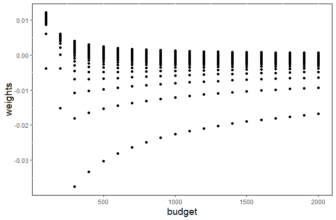
Figures 1 and 2 show the behaviors of the optimal weights for K=1K=1. Figure 1 shows that in general the weights range across positive and negative numbers, with higher concentration around 0 as the budget increases. Figure 2 shows that, against the simulation run index, the weight starts from the most negative and gradually increases to the positive region. Lastly, Table 4 shows the AMRR when q1=1,q2=1q_{1}=1,q_{2}=1 (the FFD and BFD cases) as a comparison. The AMRR in this case has the same decay rate and is smaller than that for q1=2,q2=1q_{1}=2,q_{2}=1 across all KK.

KK 0.5 0.6 0.7 0.8 0.9 1.0 1.1 1.2 1.3 1.4 1.5 1.6 1.7 1.8 1.9 2.0
AMRR 2.67 1.85 1.36 1.04 0.82 0.67 0.55 0.46 0.39 0.34 0.30 0.26 0.23 0.21 0.18 0.17
Table 3: AMRR for general weighted estimators, against KK, when q1=2,q2=1q_{1}=2,q_{2}=1
Refer to caption
Figure 1: Distribution of weights, with K=1K=1, and budget nn from 100100 to 20002000, when q1=2,q2=1q_{1}=2,q_{2}=1
Refer to caption
Figure 2: Distribution of weights against simulation step, with K=1K=1, and budget n=1000n=1000, when q1=2,q2=1q_{1}=2,q_{2}=1
KK 0.5 0.6 0.7 0.8 0.9 1.0 1.1 1.2 1.3 1.4 1.5 1.6 1.7 1.8 1.9 2.0
AMRR 2.00 1.39 1.02 0.78 0.62 0.50 0.41 0.34 0.30 0.26 0.22 0.20 0.17 0.15 0.14 0.13
Table 4: AMRR for general weighted estimators, against KK, when q1=1,q2=1q_{1}=1,q_{2}=1

5.2 Constrained Optimization for Bias-Variance Balancing

We explain intuitively the key arguments that lead to the optimal two-decay weights wj,n∗w_{j,n}^{*} and the identification of the AMRR in the form depicted in Theorem 5.1. We first note that to avoid arbitrarily large value of Rg​e​nR^{gen}, the sequence wj,nw_{j,n} must sum up to 1 (up to a vanishing error), since otherwise the scenario where θ^​(⋅)\hat{\theta}(\cdot) has no bias and noise but θ\theta is arbitrarily big will blow up Rg​e​nR^{gen}.

Thus, for simplicity let us assume that ∑j=1nwj,n=1\sum_{j=1}^{n}w_{j,n}=1. Also, for convenience, we shorthand wjw_{j} as wj,nw_{j,n}, and ww as w(n)w^{(n)} when no confusion arises. Moreover, without loss of generality, here we assume n0=0n_{0}=0 for notational convenience. Considering the bias and variance of ∑j=1nwj​θ^j​(δj)\sum_{j=1}^{n}w_{j}\hat{\theta}_{j}(\delta_{j}), we can write

MSE1g​e​n​(θ^​(⋅),d~,w)\displaystyle\text{MSE}_{1}^{gen}(\hat{\theta}(\cdot),\tilde{d},w) =\displaystyle= (∑j=1nwj​b​(δj))2+∑j=1nwj2​V​a​r​(v⁡(δj))\displaystyle\left(\sum_{j=1}^{n}w_{j}b(\delta_{j})\right)^{2}+\sum_{j=1}^{n}w_{j}^{2}Var(v(\delta_{j})) (38)
=\displaystyle= (∑j=1nwj​(B​d~q1jα​q1+o⁡(1jα​q1)))2+∑j=1nwj2​σ2​(1+o⁡(1))​j2​α​q2d~2​q2\displaystyle\left(\sum_{j=1}^{n}w_{j}\left(B\frac{\tilde{d}^{q_{1}}}{j^{\alpha q_{1}}}+o\left(\frac{1}{j^{\alpha q_{1}}}\right)\right)\right)^{2}+\sum_{j=1}^{n}w_{j}^{2}\frac{\sigma^{2}(1+o(1))j^{2\alpha q_{2}}}{\tilde{d}^{2q_{2}}}
=\displaystyle= (B​d~q1​∑j=1nwjjα​q1)2+σ2d~2​q2​∑j=1nj2​α​q2​wj2+error\displaystyle\left(B\tilde{d}^{q_{1}}\sum_{j=1}^{n}\frac{w_{j}}{j^{\alpha q_{1}}}\right)^{2}+\frac{\sigma^{2}}{\tilde{d}^{2q_{2}}}\sum_{j=1}^{n}j^{2\alpha q_{2}}w_{j}^{2}+\text{error}

Recall the discussion in Section 4.3. To control the adversary from increasing Rg​e​nR^{gen}, we attempt to maintain the relative balance of bias and variance in a similar manner as the baseline. More specifically, presuming that θ^ng​e​n\hat{\theta}_{n}^{gen} exhibits the optimal MSE order n−q1/(q1+q2)n^{-q_{1}/(q_{1}+q_{2})}, we keep the ratios of the coefficients in front of B2B^{2} and σ2\sigma^{2} of the first-order MSE terms, between θ^ng​e​n\hat{\theta}_{n}^{gen} and θ¯n\bar{\theta}_{n}, to be the same. The coefficient of the squared bias term is roughly

nq1/(q1+q2)​(d~q1​∑j=1nwjjα​q1)2n^{q_{1}/(q_{1}+q_{2})}\left(\tilde{d}^{q_{1}}\sum_{j=1}^{n}\frac{w_{j}}{j^{\alpha q_{1}}}\right)^{2}

while the coefficient of the variance term is roughly

nq1/(q1+q2)​1d~2​q2​∑j=1nj2​α​q2​wj2n^{q_{1}/(q_{1}+q_{2})}\frac{1}{\tilde{d}^{2q_{2}}}\sum_{j=1}^{n}j^{2\alpha q_{2}}w_{j}^{2}

Thus, similar to (18), we would like to ensure

nq1/(q1+q2)​((d~d)q1​∑j=1nwjjα​q1)2=nq1/(q1+q2)​1(d~d)2​q2​∑j=1nj2​α​q2​wj2n^{q_{1}/(q_{1}+q_{2})}\left(\left(\frac{\tilde{d}}{d}\right)^{q_{1}}\sum_{j=1}^{n}\frac{w_{j}}{j^{\alpha q_{1}}}\right)^{2}=n^{q_{1}/(q_{1}+q_{2})}\frac{1}{\left(\frac{\tilde{d}}{d}\right)^{2q_{2}}}\sum_{j=1}^{n}j^{2\alpha q_{2}}w_{j}^{2} (39)

Denoting η=d~/d\eta=\tilde{d}/d, and dropping nq1/(q1+q2)n^{q_{1}/(q_{1}+q_{2})} on both sides of (39), we consider the optimization problem

minw,ηSsubject toS=(ηq1​∑j=1nwjjα​q1)2=1η2​q2​∑j=1nj2​α​q2​wj2η≤K∑j=1nwj=1\begin{array}[]{ll}\min_{w,\eta}&S\\ \text{subject to}&S=\left(\eta^{q_{1}}\sum_{j=1}^{n}\frac{w_{j}}{j^{\alpha q_{1}}}\right)^{2}=\frac{1}{\eta^{2q_{2}}}\sum_{j=1}^{n}j^{2\alpha q_{2}}w_{j}^{2}\\ &\eta\leq K\\ &\sum_{j=1}^{n}w_{j}=1\end{array} (40)

Note that the first constraint is the bias-variance-balancing condition as in (19). The second and third constraints capture the inflation condition g⁡(⋅)∈ℱKg(\cdot)\in\mathcal{F}_{K} and ∑j=1nwj=1\sum_{j=1}^{n}w_{j}=1. Denote the optimal value of (40) as Sn∗S_{n}^{*}. Then roughly speaking, the AMRR would be limn→∞nq1/(q1+q2)​Sn∗\lim_{n\to\infty}n^{q_{1}/(q_{1}+q_{2})}S_{n}^{*}. The associated optimal solution w,ηw,\eta turns out to dominate any other possibilities, in particular those obtained by allowing any of the bias and variance terms dominate another.

In the rest of this subsection, we will explain how (40) leads to the two-decay representation of wj,n∗w_{j,n}^{*}, and leave other details to Appendix C. Note that (40) is non-convex. However, we can reformulate it into a convex program together with a simple one-dimensional line search over a region that consists of at most two intervals.

To this end, first notice that from the first constraint in (40), we have

η=(∑j=1nj2​α​q2​wj2(∑j=1nwjjα​q1)2)1/(2​(q1+q2))\eta=\left(\frac{\sum_{j=1}^{n}j^{2\alpha q_{2}}w_{j}^{2}}{\left(\sum_{j=1}^{n}\frac{w_{j}}{j^{\alpha q_{1}}}\right)^{2}}\right)^{1/(2(q_{1}+q_{2}))} (41)

so that the second constraint is equivalent to

∑j=1nj2​α​q2​wj2≤K2​(q1+q2)​(∑j=1nwjjα​q1)2\sum_{j=1}^{n}j^{2\alpha q_{2}}w_{j}^{2}\leq K^{2(q_{1}+q_{2})}\left(\sum_{j=1}^{n}\frac{w_{j}}{j^{\alpha q_{1}}}\right)^{2}

Moreover, by plugging in (41), the objective function of (40) becomes

|∑j=1nwjjα​q1|2​q2/(q1+q2)​(∑j=1nj2​α​q2​wj2)q1/(q1+q2)\left|\sum_{j=1}^{n}\frac{w_{j}}{j^{\alpha q_{1}}}\right|^{2q_{2}/(q_{1}+q_{2})}\left(\sum_{j=1}^{n}j^{2\alpha q_{2}}w_{j}^{2}\right)^{q_{1}/(q_{1}+q_{2})}

Therefore, (40) can be rewritten as

minw|∑j=1nwjjα​q1|2​q2/(q1+q2)​(∑j=1nj2​α​q2​wj2)q1/(q1+q2)subject to∑j=1nj2​α​q2​wj2≤K2​(q1+q2)​(∑j=1nwjjα​q1)2∑j=1nwj=1\begin{array}[]{ll}\min_{w}&\left|\sum_{j=1}^{n}\frac{w_{j}}{j^{\alpha q_{1}}}\right|^{2q_{2}/(q_{1}+q_{2})}\left(\sum_{j=1}^{n}j^{2\alpha q_{2}}w_{j}^{2}\right)^{q_{1}/(q_{1}+q_{2})}\\ \text{subject to}&\sum_{j=1}^{n}j^{2\alpha q_{2}}w_{j}^{2}\leq K^{2(q_{1}+q_{2})}\left(\sum_{j=1}^{n}\frac{w_{j}}{j^{\alpha q_{1}}}\right)^{2}\\ &\sum_{j=1}^{n}w_{j}=1\end{array} (42)

To reduce (42) into a more tractable form, we introduce the variable a=∑j=1nwjjα​q1a=\sum_{j=1}^{n}\frac{w_{j}}{j^{\alpha q_{1}}}, and write (42) as

minw,a|a|2​q2/(q1+q2)​(∑j=1nj2​α​q2​wj2)q1/(q1+q2)subject to∑j=1nj2​α​q2​wj2≤K2​(q1+q2)​a2∑j=1nwjjα​q1=a∑j=1nwj=1\begin{array}[]{ll}\min_{w,a}&|a|^{2q_{2}/(q_{1}+q_{2})}\left(\sum_{j=1}^{n}j^{2\alpha q_{2}}w_{j}^{2}\right)^{q_{1}/(q_{1}+q_{2})}\\ \text{subject to}&\sum_{j=1}^{n}j^{2\alpha q_{2}}w_{j}^{2}\leq K^{2(q_{1}+q_{2})}a^{2}\\ &\sum_{j=1}^{n}\frac{w_{j}}{j^{\alpha q_{1}}}=a\\ &\sum_{j=1}^{n}w_{j}=1\end{array}

which can be further rewritten as

mina⁡|a|2​q2/(q1+q2)​Zn∗​(a)2​q1/(q1+q2)\min_{a}|a|^{2q_{2}/(q_{1}+q_{2})}Z_{n}^{*}(a)^{2q_{1}/(q_{1}+q_{2})} (43)

where

Zn∗​(a)=minw(∑j=1nj2​α​q2​wj2)1/2subject to∑j=1nj2​α​q2​wj2≤K2​(q1+q2)​a2∑j=1nwjjα​q1=a∑j=1nwj=1\begin{array}[]{lll}Z_{n}^{*}(a)=&\min_{w}&\left(\sum_{j=1}^{n}j^{2\alpha q_{2}}w_{j}^{2}\right)^{1/2}\\ &\text{subject to}&\sum_{j=1}^{n}j^{2\alpha q_{2}}w_{j}^{2}\leq K^{2(q_{1}+q_{2})}a^{2}\\ &&\sum_{j=1}^{n}\frac{w_{j}}{j^{\alpha q_{1}}}=a\\ &&\sum_{j=1}^{n}w_{j}=1\end{array} (44)

Note that (44) is a quadratic program. We write it in a simpler form as

minw‖Σ1/2​w‖subject to‖Σ1/2​w‖2≤K2​(q1+q2)​a2μ′​w=a𝟙′​w=1\begin{array}[]{ll}\min_{w}&\|\Sigma^{1/2}w\|\\ \text{subject to}&\|\Sigma^{1/2}w\|^{2}\leq K^{2(q_{1}+q_{2})}a^{2}\\ &\mu^{\prime}w=a\\ &\mathbb{1}^{\prime}w=1\end{array} (45)

where Σ=diag​(j2​α​q2)j=1,…,n∈ℝn×n\Sigma=\text{diag}(j^{2\alpha q_{2}})_{j=1,\ldots,n}\in\mathbb{R}^{n\times n}, μ=(1/jα​q1)j=1,…,n∈ℝn\mu=(1/j^{\alpha q_{1}})_{j=1,\ldots,n}\in\mathbb{R}^{n}, 𝟙=(1)j∈ℝn\mathbb{1}=(1)_{j}\in\mathbb{R}^{n}, and ∥⋅∥\|\cdot\| is the L2L_{2}-norm. We can further separate out the first constraint in (45). To this end, denote

Z~n∗​(a)=minw‖Σ1/2​w‖subject toμ′​w=a𝟙′​w=1\begin{array}[]{lll}\tilde{Z}_{n}^{*}(a)=&\min_{w}&\|\Sigma^{1/2}w\|\\ &\text{subject to}&\mu^{\prime}w=a\\ &&\mathbb{1}^{\prime}w=1\end{array} (46)

and note that

Zn∗​(a)={Z~n∗​(a) if ​Z~n∗​(a)2≤K2​(q1+q2)​a2∞ otherwiseZ_{n}^{*}(a)=\left\{\begin{array}[]{ll}\tilde{Z}_{n}^{*}(a)&\text{\ if\ }{\tilde{Z}_{n}^{*}(a)}^{2}\leq K^{2(q_{1}+q_{2})}a^{2}\\ \infty&\text{\ otherwise}\end{array}\right. (47)

Putting in (47), optimization problem (43) becomes

mina:Z~n∗​(a)2≤K2​(q1+q2)​a2|a|2​q2/(q1+q2)Z~n∗(a)2​q1/(q1+q2)\min_{a:{\tilde{Z}_{n}^{*}(a)}^{2}\leq K^{2(q_{1}+q_{2})}a^{2}}|a|^{2q_{2}/(q_{1}+q_{2})}\tilde{Z}_{n}^{*}(a)^{2q_{1}/(q_{1}+q_{2})} (48)

Thus, our strategy to solve (40) is to first solve for an optimal solution w∗​(a)=(wj∗​(a∗))j=1,…,nw^{*}(a)=(w_{j}^{*}(a^{*}))_{j=1,\ldots,n} to (46) and obtain Z~n∗​(a)\tilde{Z}_{n}^{*}(a), and then conduct a line search for aa in (48). An optimal calibration configuration is given by the weighting sequence w∗​(a∗)w^{*}(a^{*}), where a∗a^{*} is an optimal solution to (48), and η∗\eta^{*}, where

η∗=(∑j=1nj2​α​q2​wj∗​(a∗)2(∑j=1nwj∗​(a∗)jα​q1)2)1/(2​(q1+q2))\eta^{*}=\left(\frac{\sum_{j=1}^{n}j^{2\alpha q_{2}}{w_{j}^{*}(a^{*})}^{2}}{\left(\sum_{j=1}^{n}\frac{w_{j}^{*}(a^{*})}{j^{\alpha q_{1}}}\right)^{2}}\right)^{1/(2(q_{1}+q_{2}))}

by using (41).

The two-decay characterization of the weighting sequence arises from the solution to (46). To illustrate, consider the Lagrangian

‖Σ1/2​w‖−λ1​(μ′​w−a)−λ2​(𝟙′​w−1)\|\Sigma^{1/2}w\|-\lambda_{1}(\mu^{\prime}w-a)-\lambda_{2}(\mathbb{1}^{\prime}w-1)

Differentiating with respect to ww and equating to 0, we get

Σ​w‖Σ1/2​w‖−λ1​μ−λ2​𝟙=0\frac{\Sigma w}{\|\Sigma^{1/2}w\|}-\lambda_{1}\mu-\lambda_{2}\mathbb{1}=0

which gives

w=Σ−1​(λ1​μ+λ2​𝟙)=λ1​Σ−1​μ+λ2​Σ−1​𝟙w=\Sigma^{-1}(\lambda_{1}\mu+\lambda_{2}\mathbb{1})=\lambda_{1}\Sigma^{-1}\mu+\lambda_{2}\Sigma^{-1}\mathbb{1}

for some λ1,λ2\lambda_{1},\lambda_{2} (scaled by ‖Σ1/2​w‖\|\Sigma^{1/2}w\| compared to the ones displayed before). Note that this is equivalent to

wj=λ1jα⁡(q1+2​q2)+λ2j2​α​q2w_{j}=\frac{\lambda_{1}}{j^{\alpha(q_{1}+2q_{2})}}+\frac{\lambda_{2}}{j^{2\alpha q_{2}}}

for j=1,…,nj=1,\ldots,n. This is precisely the form of wj,n∗w_{j,n}^{*} in Theorem 5.1. By identifying λ1\lambda_{1} and λ2\lambda_{2} using the constraints in (46), and writing out η∗\eta^{*} and Z~n∗​(a)\tilde{Z}_{n}^{*}(a), we arrive at the depicted choices of ww and g⁡(⋅)g(\cdot) in the theorem. The remainder of the argument comprises an analysis to show that no other choices of ww and g⁡(⋅)g(\cdot) can give a better asymptotic minimax ratio, via comparing with an alternate optimization problem, and demonstrating that the residual error induced by wj,n∗w_{j,n}^{*} and η∗\eta^{*} in (38) is indeed of higher order. Appendix C shows the details.

6 Multivariate Generalizations

All results we have presented apply to the multivariate version of (7). For convenience, we adopt the notations there. We are interested in estimating θ∈ℝp\theta\in\mathbb{R}^{p}. Given a tuning parameter δ∈ℝ+\delta\in\mathbb{R}_{+}, we can run Monte Carlo simulation where each simulation run outputs

θ^​(δ)=θ+b⁡(δ)+v⁡(δ)\hat{\theta}(\delta)=\theta+b(\delta)+v(\delta) (49)

with b⁡(δ)=B​δq1+o⁡(δq1)b(\delta)=B\delta^{q_{1}}+o(\delta^{q_{1}}) as δ→0\delta\to 0, v⁡(δ)=ε⁡(δ)δq2v(\delta)=\frac{\varepsilon(\delta)}{\delta^{q_{2}}}, and q1,q2>0q_{1},q_{2}>0. We assume that: {assumption} We have

  1. 1.

    B∈ℝpB\in\mathbb{R}^{p} is a non-zero constant vector.

  2. 2.

    ε⁡(δ)∈ℝp\varepsilon(\delta)\in\mathbb{R}^{p} is a family of random vectors such that E​ε​(δ)=0E\varepsilon(\delta)=0 and limδ→0C​o​v​(ε⁡(δ))=Σ\lim_{\delta\to 0}Cov(\varepsilon(\delta))=\Sigma for some positive semidefinite matrix Σ\Sigma with t​r​(Σ)>0tr(\Sigma)>0.

The constructions of the considered estimators are generalized in a natural manner. Namely, the sample-average-based estimator θ¯n\bar{\theta}_{n} is obtained by taking the average of nn vectors of θ^​(δ)\hat{\theta}(\delta). The recursive estimator (15) is obtained in a vectorized form, where the step size γn∈ℝ+\gamma_{n}\in\mathbb{R}_{+} is still in the form c​(n+n0)−βc(n+n_{0})^{-\beta} and δn=d~​(n+n0)−α\delta_{n}=\tilde{d}(n+n_{0})^{-\alpha}. Similar vectorization holds for the averaging estimator (16). Lastly, the general weighted estimator in (21) can also be defined in a vectorized form, with {wj,n}j=1,…,n,n=1,2,…\{w_{j,n}\}_{j=1,\ldots,n,\ n=1,2,\ldots} still a triangular array of weights.

To gauge the error of an estimator θ^n\hat{\theta}_{n}, we use the MSE given by E​‖θ^n−θ‖2E\|\hat{\theta}_{n}-\theta\|^{2}. Note that we can decompose this into bias and variance in L2L_{2}, namely ‖E​θ^n−θ‖2+t​r​(C​o​v​(θ^n))\|E\hat{\theta}_{n}-\theta\|^{2}+tr(Cov(\hat{\theta}_{n})). With this definition of MSE, the asymptotic risk ratios (12) and (14) can be similarly defined. Then all the results in Sections 3, 4 and 5 hold with only cosmetic changes. Appendices A and B show the multivariate version of the theorems and proofs in Sections 3 and 4, while it will be clear from the developments in Appendix C that the multivariate analog of Theorem 5.1 follows from its proof directly (essentially, by replacing B2B^{2} with ‖B‖2\|B\|^{2} and σ2\sigma^{2} with tr​(Σ)\text{tr}(\Sigma)).

Multivariate estimators in the form (49) arise in, for example, zeroth order gradient estimator using simultaneous perturbation (Spall 1992). To estimate ∇f​(x)\nabla f(x), a sample output would involve first simulating a random vector, say h=(hi)i=1,…,p∈ℝph=(h_{i})_{i=1,\ldots,p}\in\mathbb{R}^{p}, then generating two unbiased simulation runs f^​(x+δ​h)\hat{f}(x+\delta h) and f^​(x−δ​h)\hat{f}(x-\delta h), and finally outputting, for each direction ii,

f^​(x+δ​h)−f^​(x−δ​h)2​δ​hi\frac{\hat{f}(x+\delta h)-\hat{f}(x-\delta h)}{2\delta h_{i}} (50)

where δ>0\delta>0 is the perturbation size. This scheme satisfies (49) with q1=2,q2=1q_{1}=2,q_{2}=1 by choosing hh to have mean-zero, independent components with finite inverse second moments, and under enough smoothness conditions on ff. One can also use several variants of (50) to obtain similar conclusions, for example the one-sided version f^​(x+δ​h)/(δ​hi)\hat{f}(x+\delta h)/(\delta h_{i}) (Spall 1997), or f^​(x+δ​h)​hi/δ\hat{f}(x+\delta h)h_{i}/\delta by choosing hh to satisfy other types of conditions, as in Gaussian smoothing (Nesterov and Spokoiny 2017) or uniform sampling (Flaxman et al. 2005).

Moreover, one important application of the above multivariate estimators concerns input uncertainty quantification (e.g., Barton 2012, Henderson 2003, Chick 2006, Song et al. 2014, Lam 2016). In particular, a common estimation target in this problem is the output variance of a simulation experiment that is contributed from the statistical noises of the input models calibrated from external data sources, which is typically expressed in the form ∇ψ(x)′Λ∇ψ(x)\nabla\psi(x)^{\prime}\Lambda\nabla\psi(x) where Λ\Lambda is the sampling covariance of the estimates of the input parameter vector x∈ℝpx\in\mathbb{R}^{p}, ∇ψ​(x)\nabla\psi(x) is the gradient of the simulation performance measure with respect to xx, and ′ denotes transpose. Thus, this is in the form of G⁡(θ)G(\theta) where θ=∇ψ​(x)\theta=\nabla\psi(x) and G⁡(θ)=θ′​Λ​θG(\theta)=\theta^{\prime}\Lambda\theta. Our results applies to estimate G⁡(θ)G(\theta) with a plug-in of θ\theta and a standard application of the delta method to control the inherited error.

7 Numerical Results

We conduct a simple experiment to demonstrate the theoretical results in this paper. We consider a generic M/M/1M/M/1 queueing system. The arrival and service rates are both set to be 4, so that the system is critically loaded. We consider a transient performance measure of the expected averaged system time of the first 10 customers, and are interested in the gradient of this quantity with respect to the arrival and service rates. The true derivatives with respect to these rates are 0.09460.0946 and −0.2501-0.2501 respectively.

We consider two settings. The first setting uses CFD to estimate the derivative with respect to the arrival rate. The second setting uses simultaneous perturbation (described in Section 6), with the perturbation vector hh being independent symmetric variables on ±1\pm 1, to estimate the gradient with respect to the arrival and service rates simultaneously. In each setting, we consider three estimators: 1) the conventional sample-average-based estimator θ¯n\bar{\theta}_{n}; 2) the recursive estimator θ^nr​e​c\hat{\theta}_{n}^{rec}; and 3) the general weighted estimator θ^ng​e​n\hat{\theta}_{n}^{gen}. In θ¯n\bar{\theta}_{n}, we set δ=d(n+n0)−1/6\delta=d(n+n_{0})^{-1/6} where d=1d=1 or 22. In θ^nr​e​c\hat{\theta}_{n}^{rec}, we set c=1c=1, δj=d~(j+n0)−1/6\delta_{j}=\tilde{d}(j+n_{0})^{-1/6} for the jj-th simulation run, where d~=3−1/6d=0.83d\tilde{d}=3^{-1/6}d=0.83d. For θ^ng​e​n\hat{\theta}_{n}^{gen}, we set δj=d~(j+n0)−1/6\delta_{j}=\tilde{d}(j+n_{0})^{-1/6} where d~=η∗​d\tilde{d}=\eta^{*}d, and use weights wj,n∗w_{j,n}^{*}, with η∗\eta^{*} and wj,n∗w_{j,n}^{*} both chosen according to Theorem 5.1. We set the “burn-in” step size n0=500n_{0}=500. For θ^ng​e​n\hat{\theta}_{n}^{gen}, we further consider different values of KK from 11 to 44. We consider the run-length varying among n=104n=10^{4}, 2×1042\times 10^{4}, 3×1043\times 10^{4}, 5×1045\times 10^{4}, 8×1048\times 10^{4} and 10510^{5}.

Tables 5 and 6 show the performances of the three estimators, using d=1d=1 and d=2d=2 in the baseline estimator θ¯n\bar{\theta}_{n} respectively. The tables demonstrate both the empirical MSE of each estimator and, for θ^nr​e​c\hat{\theta}_{n}^{rec} and θ^ng​e​n\hat{\theta}_{n}^{gen}, the risk ratio compared with θ¯n\bar{\theta}_{n} (i.e., ratio between the empirical MSEs of the considered estimator and θ¯n\bar{\theta}_{n}; shown in the bracket). In each parameter configuration, the empirical MSE is calculated by independently repeating the experiment 1,0001,000 times. When d=1d=1, we see that the recursive estimator θ^nr​e​c\hat{\theta}_{n}^{rec} has generally a larger MSE compared to θ¯n\bar{\theta}_{n}, among all the budget nn we consider, with an inflation ranging from 99%99\% to 111%111\%. This is roughly consistent with the implications of Theorems 4.4 and 4.7 that the AMRR for θ^nr​e​c\hat{\theta}_{n}^{rec} in this case is 108%108\% (also shown in Table 1).

In contrast, the general weighted estimator θ^ng​e​n\hat{\theta}_{n}^{gen} has a significantly smaller MSE than θ¯n\bar{\theta}_{n}. Moreover, the risk ratio is consistent with the implication of Theorem 5.1 and Corollary 5.2. More concretely, we see that the risk ratio is estimated to be around 68−81%68-81\% when K=1K=1, and 17−21%17-21\% when K=2K=2, for our considered range of nn. Table 3 shows that the AMRR is 67%67\% when K=1K=1, and 17%17\% when K=2K=2, which largely match the experimental ratios. Moreover, these ratios appear to be quite stable for the various values of nn. However, when KK is further increased to 3 or 4, although the improvement of θ^ng​e​n\hat{\theta}_{n}^{gen} persists, we see a general deterioration in the improvement, with the risk ratio rising back to 74%74\% for K=3K=3 and 56%56\% for K=4K=4 when n=10,000n=10,000, the smallest budget we consider. Moreover, the risk ratios for K=3K=3 and K=4K=4 generally decrease with nn towards the AMRR. These hint a manifestation of finite-sample behaviors as KK is now relatively large compared to the budget nn. From Table 5, it seems that taking K=2K=2 is a safe and notably good choice.

Table 6 shows a similar pattern as Table 5, when dd is now taken to be 2. The risk ratio of θ^nr​e​c\hat{\theta}_{n}^{rec} compared to θ¯n\bar{\theta}_{n} ranges from 104%104\% to 129%129\%, which again roughly match the AMRR 108%108\% in this case. The risk ratio of θ^ng​e​n\hat{\theta}_{n}^{gen} when K=1K=1 ranges from 75%75\% to 83%83\%, while when K=2K=2 ranges from 19%19\% to 21%21\%, again roughly consistent with the AMRRs of 67%67\% and 17%17\% respectively. Like the case of d=1d=1, the improvement of θ^ng​e​n\hat{\theta}_{n}^{gen} over θ¯n\bar{\theta}_{n} persists when K=3K=3 and 44, but the improvement generally deteriorates, and in this case also becomes more variable.

nn θ¯n\bar{\theta}_{n} θ^nr​e​c\hat{\theta}_{n}^{rec} θ^ng​e​n\hat{\theta}_{n}^{gen}
K=1K=1 K=2K=2 K=3K=3 K=4K=4
10000 1.79E-4 1.97E-4 (110%) 1.21E-4 (68%) 3.05E-5 (17%) 1.32E-4 (74%) 9.98E-5 (56%)
20000 1.02E-4 1.09E-4 (107%) 8.07E-5 (79%) 1.94E-5 (19%) 7.40E-5 (73%) 4.71E-5 (46%)
30000 7.59E-5 8.31E-5 (110%) 6.12E-5 (81%) 1.59E-5 (21%) 5.03E-5 (66%) 2.71E-5 (36%)
50000 5.67E-5 6.29E-5 (111%) 4.03E-5 (71%) 1.16E-5 (20%) 2.79E-5 (49%) 1.62E-5 (29%)
80000 4.11E-5 4.34E-5 (106%) 3.10E-5 (75%) 8.21E-6 (20%) 1.94E-5 (47%) 1.00E-5 (24%)
100000 3.82E-5 3.79E-5 (99%) 2.79E-5 (73%) 7.10E-6 (19%) 1.47E-5 (39%) 8.67E-6 (23%)
Table 5: Empirical MSE among estimators for the derivative with respect to the arrival rate, d=1d=1. Bracketed numbers represent the risk ratios between the considered estimators and the baseline θ¯n\bar{\theta}_{n}.
nn θ¯n\bar{\theta}_{n} θ^nr​e​c\hat{\theta}_{n}^{rec} θ^ng​e​n\hat{\theta}_{n}^{gen}
K=1K=1 K=2K=2 K=3K=3 K=4K=4
10000 4.38E-5 4.64E-5 (106%) 3.47E-5 (79%) 8.28E-6 (19%) 3.73E-6 (9%) 2.83E-5 (65%)
20000 2.43E-5 2.71E-5 (112%) 1.85E-5 (76%) 4.73E-6 (19%) 2.14E-6 (9%) 1.78E-5 (73%)
30000 1.91E-5 2.45E-5 (129%) 1.57E-5 (83%) 3.96E-6 (21%) 1.74E-5 (91%) 1.18E-5 (62%)
50000 1.54E-5 1.60E-5 (104%) 1.18E-5 (77%) 2.87E-6 (19%) 9.79E-6 (63%) 6.03E-6 (39%)
80000 1.11E-5 1.21E-5 (109%) 8.52E-6 (77%) 2.13E-6 (19%) 5.79E-6 (52%) 4.18E-6 (38%)
100000 9.19E-6 1.08E-5 (117%) 6.88E-6 (75%) 1.77E-6 (19%) 5.44E-6 (59%) 3.58E-6 (39%)
Table 6: Empirical MSE among estimators for the derivative with respect to the arrival rate, d=2d=2. Bracketed numbers represent the risk ratios between the considered estimators and the baseline θ¯n\bar{\theta}_{n}.

In the second set of experiments, we test the gradient estimator for both the arrival and service rates using simultaneous perturbation. Tables 7 and 8 show the performances of θ^nr​e​c\hat{\theta}_{n}^{rec} and θ^ng​e​n\hat{\theta}_{n}^{gen} relative to θ¯n\bar{\theta}_{n} when d=1d=1 and d=2d=2 respectively. We use K=1K=1 or 22 in θ^ng​e​n\hat{\theta}_{n}^{gen}, as they are observed to perform reasonably well in the single-variate case. We see that θ^nr​e​c\hat{\theta}_{n}^{rec} continues to have generally a larger MSE than θ¯n\bar{\theta}_{n}, with risk ratios ranging from 100%100\% to 115%115\% when d=1d=1 and 103%103\% to 115%115\% when d=2d=2 for the considered budgets, which are consistent with the AMRR of 108%108\%. When d=1d=1, the risk ratios of θ^ng​e​n\hat{\theta}_{n}^{gen} range from 71%71\% to 83%83\% for K=1K=1, and improve to 35%35\% to 46%46\% for K=2K=2. When d=2d=2, the risk ratios of θ^ng​e​n\hat{\theta}_{n}^{gen} range from 94%94\% to 102%102\% for K=1K=1, and from 57%57\% to 67%67\% for K=2K=2. These trends are consistent with the AMRR for K=1K=1 and K=2K=2 respectively, although the experimental numbers seem to increase generally and are above the theoretical calculation as dd increases. Lastly, the risk ratios across different nn in the considered range seem to be quite stable, hinting that these budgets are sufficient to observe the studied asymptotic behaviors in this case.

nn θ¯n\bar{\theta}_{n} θ^nr​e​c\hat{\theta}_{n}^{rec} θ^ng​e​n\hat{\theta}_{n}^{gen}
K=1K=1 K=2K=2
10000 1.69E-4 1.94E-4 (115%) 1.35E-4 (80%) 6.62E-5 (39%)
20000 1.13E-4 1.26E-4 (112%) 8.60E-5 (76%) 4.45E-5 (39%)
30000 9.40E-5 9.41E-5 (100%) 6.70E-5 (71%) 3.33E-5 (35%)
50000 5.99E-5 6.08E-5 (102%) 4.70E-5 (78%) 2.56E-5 (43%)
80000 4.62E-5 5.30E-5 (115%) 3.52E-5 (76%) 1.92E-5 (41%)
100000 3.83E-5 4.29E-5 (112%) 3.17E-5 (83%) 1.77E-5 (46%)
Table 7: Empirical MSE among estimators for the gradient with respect to the arrival and service rates, d=1d=1. Bracketed numbers represent the risk ratios between the considered estimators and the baseline θ¯n\bar{\theta}_{n}
nn θ¯n\bar{\theta}_{n} θ^nr​e​c\hat{\theta}_{n}^{rec} θ^ng​e​n\hat{\theta}_{n}^{gen}
K=1K=1 K=2K=2
10000 5.85E-5 6.28E-5 (107%) 5.50E-5 (94%) 3.35E-5 (57%)
20000 3.27E-5 3.76E-5 (115%) 3.33E-5 (102%) 2.19E-5 (67%)
30000 2.67E-5 2.82E-5 (106%) 2.52E-5 (94%) 1.65E-5 (62%)
50000 1.85E-5 2.00E-5 (108%) 1.81E-5 (98%) 1.16E-5 (63%)
80000 1.36E-5 1.40E-5 (103%) 1.30E-5 (96%) 8.06E-6 (59%)
100000 1.18E-5 1.26E-5 (107%) 1.10E-5 (94%) 6.73E-6 (57%)
Table 8: Empirical MSE among estimators for the gradient with respect to the arrival and service rates, d=2d=2. Bracketed numbers represent the risk ratios between the considered estimators and the baseline θ¯n\bar{\theta}_{n}

8 Conclusion

We have studied a framework to construct new estimators that, in situations where simulation runs are biased for a target estimation quantity, consistently outperform baseline estimators as the sample averages of the simulation runs with a chosen tuning parameter. One challenge in choosing the latter lies in the often lack of knowledge on the model characteristics that affect the bias-variance tradeoff. To mitigate the adversarial impact of this ambiguity, we propose a minimax analysis on the asymptotic risk ratio that compares the mean square errors between proposed estimators and the baseline. In particular, we identify the asymptotic minimax risk ratio (AMRR) and the optimal configurations for recursive estimators and their standard averaging versions. We show that, in typical cases, the AMRR for these estimators are not small enough to justify any outperformance against the standard baseline. We then consider a more general class of weighted estimators, and identify the AMRR that can be significantly reduced to a level that implies that the resulting optimal estimator asymptotically outperforms the baseline, regardless of any realizations of the unknown model characteristics. Moreover, we provide an explicit characterizations of the optimal weights in a two-decay-rate form, and argue how this arises from a balancing of bias-variance that matches the baseline in order to control an adversarial enlargement of the risk ratio.

Our work opens the door to multiple lines of expansion, in terms of both the formulating framework and the techniques. For example, our approach can be used to find better estimators for problems where simulation runtime is significantly affected by the tuning parameters, in addition to bias and variance. This arises in the discretization schemes in, e.g., the simulation of stochastic differential equations. The statistical inference and construction of confidence intervals/regions of our weighted estimators, which involves analyzing central limit behaviors and the proper design of data-driven schemes like sectioning, are also of interest. Lastly, we plan to study our enhanced estimators, in the context of finite-differences for zeroth-order gradient estimation, for iterative algorithms in black-box stochastic optimization.

Acknowledgments.
We gratefully acknowledge support from the National Science Foundation under grants CMMI-1542020, CMMI-1523453 and CAREER CMMI-1653339/1834710.

References

  • Agrawal et al. (2012) Agrawal S, Ding Y, Saberi A, Ye Y (2012) Price of correlations in stochastic optimization. Operations Research 60(1):150–162.
  • Asmussen and Glynn (2007) Asmussen S, Glynn PW (2007) Stochastic simulation: algorithms and analysis, volume 57 (Springer Science & Business Media).
  • Barton (2012) Barton RR (2012) Input uncertainty in outout analysis. Proceedings of the Winter Simulation Conference, 6 (Winter Simulation Conference).
  • Ben-Tal et al. (2009) Ben-Tal A, El Ghaoui L, Nemirovski A (2009) Robust optimization, volume 28 (Princeton University Press).
  • Ben-Tal and Nemirovski (2002) Ben-Tal A, Nemirovski A (2002) Robust optimization–methodology and applications. Mathematical Programming 92(3):453–480.
  • Bertsimas et al. (2011) Bertsimas D, Brown DB, Caramanis C (2011) Theory and applications of robust optimization. SIAM review 53(3):464–501.
  • Besbes and Zeevi (2009) Besbes O, Zeevi A (2009) Dynamic pricing without knowing the demand function: Risk bounds and near-optimal algorithms. Operations Research 57(6):1407–1420.
  • Besbes and Zeevi (2011) Besbes O, Zeevi A (2011) On the minimax complexity of pricing in a changing environment. Operations research 59(1):66–79.
  • Blanchet and Glynn (2015) Blanchet JH, Glynn PW (2015) Unbiased monte carlo for optimization and functions of expectations via multi-level randomization. Winter Simulation Conference (WSC), 2015, 3656–3667 (IEEE).
  • Borkar (2009) Borkar VS (2009) Stochastic approximation: a dynamical systems viewpoint, volume 48 (Springer).
  • Cesa-Bianchi and Lugosi (2006) Cesa-Bianchi N, Lugosi G (2006) Prediction, learning, and games (Cambridge university press).
  • Chick (2006) Chick SE (2006) Bayesian ideas and discrete event simulation: why, what and how. Proceedings of the 38th conference on Winter simulation, 96–105 (Winter Simulation Conference).
  • Chung (1954) Chung KL (1954) On a stochastic approximation method. The Annals of Mathematical Statistics 463–483.
  • Duplay et al. (2018) Duplay D, Lam H, Zhang X (2018) Achieving optimal bias-variance tradeoff in online derivative estimation. Winter Simulation Conference (WSC), 2018 (IEEE).
  • Fabian (1967) Fabian V (1967) Stochastic approximation of minima with improved asymptotic speed. The Annals of Mathematical Statistics 191–200.
  • Fabian (1968) Fabian V (1968) On asymptotic normality in stochastic approximation. The Annals of Mathematical Statistics 39(4):1327–1332.
  • Flaxman et al. (2005) Flaxman AD, Kalai AT, McMahan HB (2005) Online convex optimization in the bandit setting: gradient descent without a gradient. Proceedings of the sixteenth annual ACM-SIAM symposium on Discrete algorithms, 385–394 (Society for Industrial and Applied Mathematics).
  • Fox and Glynn (1989) Fox BL, Glynn PW (1989) Replication schemes for limiting expectations. Probability in the Engineering and Informational Sciences 3(3):299–318.
  • Fu (2006) Fu MC (2006) Gradient estimation. Handbooks in operations research and management science 13:575–616.
  • Fu et al. (2009) Fu MC, Hong LJ, Hu JQ (2009) Conditional monte carlo estimation of quantile sensitivities. Management Science 55(12):2019–2027.
  • Fu and Hu (1992) Fu MC, Hu JQ (1992) Extensions and generalizations of smoothed perturbation analysis in a generalized semi-markov process framework. IEEE Transactions on Automatic Control 37(10):1483–1500.
  • Giles (2008) Giles MB (2008) Multilevel monte carlo path simulation. Operations Research 56(3):607–617.
  • Glasserman (2013) Glasserman P (2013) Monte Carlo methods in financial engineering, volume 53 (Springer Science & Business Media).
  • Glasserman and Gong (1990) Glasserman P, Gong WB (1990) Smoothed perturbation analysis for a class of discrete-event systems. IEEE Transactions on Automatic Control 35(11):1218–1230.
  • Glynn (1990) Glynn PW (1990) Likelihood ratio gradient estimation for stochastic systems. Communications of the ACM 33(10):75–84.
  • Glynn and Whitt (1992) Glynn PW, Whitt W (1992) The asymptotic efficiency of simulation estimators. Operations research 40(3):505–520.
  • Gong and Ho (1987) Gong WB, Ho YC (1987) Smoothed (conditional) perturbation analysis of discrete event dynamical systems. IEEE Transactions on Automatic Control 32(10):858–866.
  • Hazan et al. (2016) Hazan E, et al. (2016) Introduction to online convex optimization. Foundations and Trends® in Optimization 2(3-4):157–325.
  • Heidelberger et al. (1988) Heidelberger P, Cao XR, Zazanis MA, Suri R (1988) Convergence properties of infinitesimal perturbation analysis estimates. Management Science 34(11):1281–1302.
  • Heidergott et al. (2010) Heidergott B, Pflug G, Farenhorst-Yuan T, et al. (2010) Gradient estimation for discrete-event systems by measure-valued differentiation. ACM Transactions on Modeling and Computer Simulation (TOMACS) 20(1):5.
  • Heidergott and Vázquez-Abad (2008) Heidergott B, Vázquez-Abad FJ (2008) Measure-valued differentiation for markov chains. Journal of Optimization Theory and Applications 136(2):187–209.
  • Henderson (2003) Henderson SG (2003) Input model uncertainty: Why do we care and what should we do about it? Proceedings of the 35th conference on Winter simulation: driving innovation, 90–100 (Winter Simulation Conference).
  • Ho et al. (1983) Ho YC, Cao X, Cassandras C (1983) Infinitesimal and finite perturbation analysis for queueing networks. Automatica 19(4):439–445.
  • Hong (2009) Hong LJ (2009) Estimating quantile sensitivities. Operations research 57(1):118–130.
  • Kushner and Yin (2003) Kushner H, Yin GG (2003) Stochastic approximation and recursive algorithms and applications, volume 35 (Springer Science & Business Media).
  • Lam (2016) Lam H (2016) Advanced tutorial: Input uncertainty and robust analysis in stochastic simulation. Winter Simulation Conference (WSC), 2016, 178–192 (IEEE).
  • L’Ecuyer (1990) L’Ecuyer P (1990) A unified view of the ipa, sf, and lr gradient estimation techniques. Management Science 36(11):1364–1383.
  • L’Ecuyer (1991) L’Ecuyer P (1991) An overview of derivative estimation. Simulation Conference, 1991. Proceedings., Winter, 207–217 (IEEE).
  • McLeish (2010) McLeish D (2010) A general method for debiasing a monte carlo estimator. arXiv preprint arXiv:1005.2228 .
  • Nemirovski et al. (2009) Nemirovski A, Juditsky A, Lan G, Shapiro A (2009) Robust stochastic approximation approach to stochastic programming. SIAM Journal on optimization 19(4):1574–1609.
  • Nesterov and Spokoiny (2017) Nesterov Y, Spokoiny V (2017) Random gradient-free minimization of convex functions. Foundations of Computational Mathematics 17(2):527–566.
  • Pasupathy (2010) Pasupathy R (2010) On choosing parameters in retrospective-approximation algorithms for stochastic root finding and simulation optimization. Operations Research 58(4-part-1):889–901.
  • Pasupathy and Kim (2011) Pasupathy R, Kim S (2011) The stochastic root-finding problem: Overview, solutions, and open questions. ACM Transactions on Modeling and Computer Simulation (TOMACS) 21(3):19.
  • Peng et al. (2018) Peng Y, Fu MC, Hu JQ, Heidergott B (2018) A new unbiased stochastic derivative estimator for discontinuous sample performances with structural parameters. Operations Research 66(2):487–499.
  • Polyak and Juditsky (1992) Polyak BT, Juditsky AB (1992) Acceleration of stochastic approximation by averaging. SIAM Journal on Control and Optimization 30(4):838–855.
  • Reiman and Weiss (1989) Reiman MI, Weiss A (1989) Sensitivity analysis for simulations via likelihood ratios. Operations Research 37(5):830–844.
  • Rhee and Glynn (2015) Rhee Ch, Glynn PW (2015) Unbiased estimation with square root convergence for sde models. Operations Research 63(5):1026–1043.
  • Rubinstein (1986) Rubinstein RY (1986) The score function approach for sensitivity analysis of computer simulation models. Mathematics and Computers in Simulation 28(5):351–379.
  • Rubinstein (1992) Rubinstein RY (1992) Sensitivity analysis of discrete event systems by the “push out” method. Annals of Operations Research 39(1):229–250.
  • Ruppert (1988) Ruppert D (1988) Efficient estimations from a slowly convergent robbins-monro process. Technical report, Cornell University Operations Research and Industrial Engineering.
  • Rychlik (1990) Rychlik T (1990) Unbiased nonparametric estimation of the derivative of the mean. Statistics & probability letters 10(4):329–333.
  • Shalev-Shwartz et al. (2012) Shalev-Shwartz S, et al. (2012) Online learning and online convex optimization. Foundations and Trends® in Machine Learning 4(2):107–194.
  • Song et al. (2014) Song E, Nelson BL, Pegden CD (2014) Advanced tutorial: Input uncertainty quantification. Simulation Conference (WSC), 2014 Winter, 162–176 (IEEE).
  • Spall (1992) Spall JC (1992) Multivariate stochastic approximation using a simultaneous perturbation gradient approximation. IEEE transactions on automatic control 37(3):332–341.
  • Spall (1997) Spall JC (1997) A one-measurement form of simultaneous perturbation stochastic approximation. Automatica 33(1):109–112.
  • Zazanis and Suri (1993) Zazanis MA, Suri R (1993) Convergence rates of finite-difference sensitivity estimates for stochastic systems. Operations research 41(4):694–703.
  • Zhou and Doyle (1998) Zhou K, Doyle JC (1998) Essentials of robust control, volume 104 (Prentice hall Upper Saddle River, NJ).

Appendix A Proofs for Section 3

We will prove a multivariate version of Theorem 3.1.

Theorem A.1

Under Assumption 6, suppose that limn→∞δ​nα=d>0\lim_{n\to\infty}\delta n^{\alpha}=d>0, the sample-average-based estimator θ¯n\bar{\theta}_{n} exhibits the asymptotic MSE

E​‖θ¯n−θ‖2=d2​q1​‖B‖2​n−2​α​q1+t​r​(Σ)d2​q2​n2​α​q2−1+o⁡(n−2​α​q1+n2​α​q2−1)​ as ​n→∞E\|\bar{\theta}_{n}-\theta\|^{2}=d^{2q_{1}}\|B\|^{2}n^{-2\alpha q_{1}}+\frac{tr(\Sigma)}{d^{2q_{2}}}n^{2\alpha q_{2}-1}+o(n^{-2\alpha q_{1}}+n^{2\alpha q_{2}-1})\textrm{ as }n\to\infty

Choosing α=1/(2​(q1+q2))\alpha=1/(2(q_{1}+q_{2})) achieves the optimal MSE order, and the asymptotic MSE is

E∥θ¯n−θ∥2=(d2​q1∥B∥2+t​r​(Σ)d2​q2)n−q1/(q1+q2)+o(n−q1/(q1+q2)) as n→∞E\|\bar{\theta}_{n}-\theta\|^{2}=\big(d^{2q_{1}}\|B\|^{2}+\frac{tr(\Sigma)}{d^{2q_{2}}}\big)n^{-q_{1}/(q_{1}+q_{2})}+o(n^{-q_{1}/(q_{1}+q_{2})})\text{ as }n\to\infty
Proof A.2

Proof of theorem A.1. By the bias-variance decomposition, we have

E​‖θ¯n−θ‖2\displaystyle E\|\bar{\theta}_{n}-\theta\|^{2} =‖E​θ¯n−θ‖2+t​r​(C​o​v​(θ¯n))\displaystyle=\|E\bar{\theta}_{n}-\theta\|^{2}+tr(Cov(\bar{\theta}_{n}))
=‖b⁡(δ)‖2+1n​t​r​(C​o​v​(v⁡(δ)))\displaystyle=\|b(\delta)\|^{2}+\frac{1}{n}tr(Cov(v(\delta)))
=‖B‖2​δ2​q1+o⁡(δ2​q1)+1n​t​r​(Σ)+o⁡(1)δ2​q2\displaystyle=\|B\|^{2}\delta^{2q_{1}}+o(\delta^{2q_{1}})+\frac{1}{n}\frac{tr(\Sigma)+o(1)}{\delta^{2q_{2}}}

Setting δ=d+o⁡(1)nα\delta=\frac{d+o(1)}{n^{\alpha}}, we obtain

E​‖θ¯n−θ‖2\displaystyle E\|\bar{\theta}_{n}-\theta\|^{2} =‖B‖2​(d+o⁡(1))2​q1n2​α​q1+o⁡(n−2​α​q1)+t​r​(Σ)+o⁡(1)(d+o⁡(1))2​q2​n2​α​q2−1\displaystyle=\|B\|^{2}\frac{(d+o(1))^{2q_{1}}}{n^{2\alpha q_{1}}}+o(n^{-2\alpha q_{1}})+\frac{tr(\Sigma)+o(1)}{(d+o(1))^{2q_{2}}}n^{2\alpha q_{2}-1}
=(‖B‖2​d2​q1+o⁡(1))​n−2​α​q1+(t​r​(Σ)d2​q2+o⁡(1))​n2​α​q2−1\displaystyle=\left(\|B\|^{2}d^{2q_{1}}+o(1)\right)n^{-2\alpha q_{1}}+\left(\frac{tr(\Sigma)}{d^{2q_{2}}}+o(1)\right)n^{2\alpha q_{2}-1}

To achieve the optimal MSE order, we solve −2​α​q1=2​α​q2−1-2\alpha q_{1}=2\alpha q_{2}-1. Thus α=1/(2​(q1+q2))\alpha=1/(2(q_{1}+q_{2})) and the optimal order is n−q1/(q1+q2)n^{-q_{1}/(q_{1}+q_{2})}. □\square

Proof A.3

Proof of Theorem 3.1. The proof follows immediately by considering dimension 1 in Theorem A.1. □\square

Appendix B Proofs for Section 4.2

We provide and prove multivariate versions of the results, from which the ones in Section 4.2 follow immediately.

Frequently used in the subsequent proofs is the following result adapted from Lemma 4.2, a version of Chung’s Lemma, in Fabian 1967:

Lemma B.1 (Chung’s Lemma)

For vn,cn,bnv_{n},c_{n},b_{n} real numbers, and 0<α≤10<\alpha\leq 1, suppose limn→∞cn=c>0\lim_{n\to\infty}c_{n}=c>0, and consider the iteration

vn+1=(1−cnnα)​vn+bnnαv_{n+1}=(1-\frac{c_{n}}{n^{\alpha}})v_{n}+\frac{b_{n}}{n^{\alpha}} (51)

If bn→0b_{n}\to 0, then vn→0v_{n}\to 0; if bn→b>0b_{n}\to b>0, then vn→b/cv_{n}\to b/c; and if bn→∞b_{n}\to\infty, then vn→∞v_{n}\to\infty.

Proof B.2

Proof of Lemma B.1. Our version of Chung’s lemma is different in appearance from Lemma 4.2 in Fabian 1968, and thus we repeat the proof here. First, if bn→bb_{n}\to b where b≥0b\geq 0 is a real number, then for given 0<ϵ<c0<\epsilon<c, we can choose n1n_{1} sufficiently large such that, for all n≥n1n\geq n_{1}, we have cnnα<1\frac{c_{n}}{n^{\alpha}}<1, bn<b+ϵb_{n}<b+\epsilon and c−ϵ<cn<c+ϵc-\epsilon<c_{n}<c+\epsilon. Now let n≥n1n\geq n_{1}. If vn≥b+2​ϵc−ϵv_{n}\geq\frac{b+2\epsilon}{c-\epsilon}, then from the iteration (51)

vn+1≤vn−b+2​ϵc−ϵ​(c−ϵ)​1nα+(b+ϵ)​1nα≤vn−ϵnαv_{n+1}\leq v_{n}-\frac{b+2\epsilon}{c-\epsilon}(c-\epsilon)\frac{1}{n^{\alpha}}+(b+\epsilon)\frac{1}{n^{\alpha}}\leq v_{n}-\frac{\epsilon}{n^{\alpha}}

On the other hand, if vn≤b+2​ϵc−ϵv_{n}\leq\frac{b+2\epsilon}{c-\epsilon}, then since the right hand side of the iteration (51) is an increasing function of vnv_{n}, we have

vn+1≤b+2​ϵc−ϵ−b+2​ϵc−ϵ​(c−ϵ)​1nα+(b+ϵ)​1nα≤b+2​ϵc−ϵv_{n+1}\leq\frac{b+2\epsilon}{c-\epsilon}-\frac{b+2\epsilon}{c-\epsilon}(c-\epsilon)\frac{1}{n^{\alpha}}+(b+\epsilon)\frac{1}{n^{\alpha}}\leq\frac{b+2\epsilon}{c-\epsilon}

Combined with the fact that ∑n=1∞1nα\sum\limits_{n=1}^{\infty}\frac{1}{n^{\alpha}} diverges, we have lim supn→∞vn≤b+2​ϵc−ϵ\limsup_{n\to\infty}v_{n}\leq\frac{b+2\epsilon}{c-\epsilon}. Since ϵ\epsilon is arbitrary, we get

lim supn→∞vn≤bc\limsup_{n\to\infty}v_{n}\leq\frac{b}{c} (52)

If b=0b=0, vn+1≥vn+ϵnαv_{n+1}\geq v_{n}+\frac{\epsilon}{n^{\alpha}} for vn≤−2​ϵc−ϵv_{n}\leq-\frac{2\epsilon}{c-\epsilon} and vn+1≥−2​ϵc−ϵv_{n+1}\geq-\frac{2\epsilon}{c-\epsilon} for vn≥−2​ϵc−ϵv_{n}\geq-\frac{2\epsilon}{c-\epsilon}. Therefore we have lim infn→∞vn≥0\liminf\limits_{n\rightarrow\infty}v_{n}\geq 0 and lim supn→∞vn≤0\limsup\limits_{n\rightarrow\infty}v_{n}\leq 0. We conclude that limn→∞vn=0\lim_{n\to\infty}v_{n}=0. By the same analysis, if bn→b>0b_{n}\to b>0, where bb possibly take the value of ∞\infty, we would have

lim infn→∞vn≥bc\liminf_{n\to\infty}v_{n}\geq\frac{b}{c} (53)

Thus if b=∞b=\infty, we conclude that limn→∞vn→∞\lim_{n\to\infty}v_{n}\to\infty, and if 0<b<∞0<b<\infty, combining (52) and (53), we get limn→∞vn=bc\lim_{n\to\infty}v_{n}=\frac{b}{c}. □\square

We now consider multivariate versions of our results and their proofs:

Proposition B.3

Under Assumption 6, we have:

  1. 1.

    If β≤1\beta\leq 1 and α<β/(2​q2)\alpha<\beta/(2q_{2}), the estimator θ^nr​e​c\hat{\theta}_{n}^{rec} is L2L_{2}-consistent for θ\theta, i.e.,

    limn→∞E​‖θ^nr​e​c−θ‖2=0\lim_{n\to\infty}E\|\hat{\theta}_{n}^{rec}-\theta\|^{2}=0
  2. 2.

    If β≤1\beta\leq 1 and α≥β/(2​q2)\alpha\geq\beta/(2q_{2}), or if β>1\beta>1, the error of θ^nr​e​c\hat{\theta}_{n}^{rec} in estimating θ\theta is bounded away from zero in L2L_{2} norm as n→∞n\to\infty, i.e.,

    lim infn→∞E​‖θ^nr​e​c−θ‖2>0\liminf_{n\to\infty}E\|\hat{\theta}_{n}^{rec}-\theta\|^{2}>0
Proof B.4

Proof of Proposition B.3. We first prove the proposition for β≤1\beta\leq 1. From the recursion

θ^nr​e​c=(1−γn)​θ^n−1r​e​c+γn​θ^​(δn)\hat{\theta}_{n}^{rec}=(1-\gamma_{n})\hat{\theta}_{n-1}^{rec}+\gamma_{n}\hat{\theta}(\delta_{n}) (54)

we have

E​θ^nr​e​c−θ=(1−γn)​(E​θ^n−1r​e​c−θ)+γn​(E​θ^​(δn)−θ)E\hat{\theta}_{n}^{rec}-\theta=(1-\gamma_{n})\left(E\hat{\theta}_{n-1}^{rec}-\theta\right)+\gamma_{n}\left(E\hat{\theta}(\delta_{n})-\theta\right)

Since E​θ^​(δn)−θ=b⁡(δn)→0​ as ​n→∞E\hat{\theta}(\delta_{n})-\theta=b(\delta_{n})\to 0\text{ as }n\to\infty, we have E​θ^nr​e​c−θ→0E\hat{\theta}_{n}^{rec}-\theta\to 0 by Chung’s lemma. Note that E​‖θ^nr​e​c−θ‖2=‖E​θ^nr​e​c−θ‖2+t​r​(C​o​v​(θ^nr​e​c))E\|\hat{\theta}_{n}^{rec}-\theta\|^{2}=\|E\hat{\theta}_{n}^{rec}-\theta\|^{2}+tr(Cov(\hat{\theta}_{n}^{rec})). Thus the convergence will depend on the variance term. Taking covariance of (54), by independence we have

C​o​v​(θ^nr​e​c)=(1−γn)2​C​o​v​(θ^n−1r​e​c)+γn2​C​o​v​(θ^​(δn))Cov(\hat{\theta}_{n}^{rec})=(1-\gamma_{n})^{2}Cov(\hat{\theta}_{n-1}^{rec})+\gamma_{n}^{2}Cov(\hat{\theta}(\delta_{n})) (55)

Since

C​o​v​(θ^​(δn))=1δn2​q2​C​o​v​(ϵ⁡(δn))Cov(\hat{\theta}(\delta_{n}))=\frac{1}{\delta_{n}^{2q_{2}}}Cov(\epsilon(\delta_{n}))

we have

limn→∞C​o​v​(θ^​(δn))n2​q2​α=Σd2​q2\lim_{n\to\infty}\frac{Cov(\hat{\theta}(\delta_{n}))}{n^{2q_{2}\alpha}}=\frac{\Sigma}{d^{2q_{2}}}

We now rewrite the iteration (55) as

t​r​(C​o​v​(θ^nr​e​c))=(1−(2+o⁡(1))​γn)​t​r​(C​o​v​(θ^n−1r​e​c))+γn​sntr(Cov(\hat{\theta}_{n}^{rec}))=(1-(2+o(1))\gamma_{n})tr(Cov(\hat{\theta}_{n-1}^{rec}))+\gamma_{n}s_{n}

where sn=c​t​r​(Σ)d2​q2​n2​q2​α−β+o⁡(n2​q2​α−β)s_{n}=c\frac{tr(\Sigma)}{d^{2q_{2}}}n^{2q_{2}\alpha-\beta}+o(n^{2q_{2}\alpha-\beta}). We note that limn→∞sn=∞\lim_{n\to\infty}s_{n}=\infty if α>β/(2​q2)\alpha>\beta/(2q_{2}), limn→∞sn=c​t​r​(Σ)d2​q2>0\lim_{n\to\infty}s_{n}=c\frac{tr(\Sigma)}{d^{2q_{2}}}>0 if α=β/(2​q2)\alpha=\beta/(2q_{2}), and limn→∞sn=0\lim_{n\to\infty}s_{n}=0 if α<β/(2​q2)\alpha<\beta/(2q_{2}). Thus by Chung’s lemma

limn→∞t​r​(C​o​v​(θ^nr​e​c))→∞​ if ​α>β/(2​q2)\lim_{n\to\infty}tr(Cov(\hat{\theta}_{n}^{rec}))\to\infty\textrm{ if }\alpha>\beta/(2q_{2})
limn→∞t​r​(C​o​v​(θ^nr​e​c))=c​t​r​(Σ)2​d2​q2​ if ​α=β/(2​q2)\lim_{n\to\infty}tr(Cov(\hat{\theta}_{n}^{rec}))=c\frac{tr(\Sigma)}{2d^{2q_{2}}}\textrm{ if }\alpha=\beta/(2q_{2})

and

limn→∞t​r​(C​o​v​(θ^nr​e​c))=0​ if ​α<β/(2​q2)\lim_{n\to\infty}tr(Cov(\hat{\theta}_{n}^{rec}))=0\textrm{ if }\alpha<\beta/(2q_{2})

This completes the proof for β≤1\beta\leq 1.

Next consider β>1\beta>1, we now argue that choosing γn=c/nβ\gamma_{n}=c/n^{\beta} does not lead to convergence. We note that θ^nr​e​c\hat{\theta}_{n}^{rec} is a linear combination of θ^0r​e​c,θ^i​(δi),i=1,⋯,n\hat{\theta}_{0}^{rec},\hat{\theta}_{i}(\delta_{i}),i=1,\cdots,n, i.e.

θ^nr​e​c=a0​θ^0r​e​c+∑i=1nai​θ^i​(δi)\hat{\theta}_{n}^{rec}=a_{0}\hat{\theta}_{0}^{rec}+\sum_{i=1}^{n}a_{i}\hat{\theta}_{i}(\delta_{i})

where a0=∏j=1n(1−γj)a_{0}=\prod_{j=1}^{n}(1-\gamma_{j}) and ai=γi​∏j=i+1n(1−γj)a_{i}=\gamma_{i}\prod_{j=i+1}^{n}(1-\gamma_{j}). Since ∑n=1∞γn=∑n=1∞cnβ<∞\sum_{n=1}^{\infty}\gamma_{n}=\sum_{n=1}^{\infty}\frac{c}{n^{\beta}}<\infty, by the relation between infinite product and infinite sum, we get

limn→∞ai​ exists and is positive for any ​i\lim_{n\to\infty}a_{i}\textrm{ exists and is positive for any }i

Since by independence

t​r​(C​o​v​(θ^nr​e​c))=a02​t​r​(C​o​v​(θ^0r​e​c))+∑i=1nai2​t​r​(C​o​v​(θ^​(δi)))tr(Cov(\hat{\theta}_{n}^{rec}))=a_{0}^{2}tr(Cov(\hat{\theta}_{0}^{rec}))+\sum_{i=1}^{n}a_{i}^{2}tr(Cov(\hat{\theta}(\delta_{i})))

we have that

lim infn→∞t​r​(C​o​v​(θ^nr​e​c))>0\liminf_{n\to\infty}tr(Cov(\hat{\theta}_{n}^{rec}))>0

□\square

Theorem B.5

Under Assumption 6, the MSE of θ^nr​e​c\hat{\theta}_{n}^{rec} in estimating θ\theta behaves as follows:

  1. 1.

    For β<1\beta<1 and α<β/(2​q2)\alpha<\beta/(2q_{2}),

    E​‖θ^nr​e​c−θ‖2=d2​q1​‖B‖2​n−2​q1​α+c2​d2​q2​t​r​(Σ)​n2​q2​α−β+o⁡(n−2​q1​α+n2​q2​α−β)​ as ​n→∞E\|\hat{\theta}_{n}^{rec}-\theta\|^{2}=d^{2q_{1}}\|B\|^{2}n^{-2q_{1}\alpha}+\frac{c}{2d^{2q_{2}}}tr(\Sigma)n^{2q_{2}\alpha-\beta}+o(n^{-2q_{1}\alpha}+n^{2q_{2}\alpha-\beta})\text{ as }n\to\infty
  2. 2.

    For β=1\beta=1, α=1/(2​(q1+q2))\alpha=1/(2(q_{1}+q_{2})) and c>q1/(2​(q1+q2))c>q_{1}/(2(q_{1}+q_{2})),

    E∥θ^nr​e​c−θ∥2=((c​dq1c−q1/(2​(q1+q2)))2∥B∥2+c2(2​c−q1/(q1+q2))​d2​q2tr(Σ))n−q1/(q1+q2)+o(n−q1/(q1+q2)) as n→∞E\|\hat{\theta}_{n}^{rec}-\theta\|^{2}=\left(\big(\frac{cd^{q_{1}}}{c-q_{1}/(2(q_{1}+q_{2}))}\big)^{2}\|B\|^{2}+\frac{c^{2}}{(2c-q_{1}/(q_{1}+q_{2}))d^{2q_{2}}}tr(\Sigma)\right)n^{-q_{1}/(q_{1}+q_{2})}+o(n^{-q_{1}/(q_{1}+q_{2})})\text{ as }n\to\infty
  3. 3.

    For β=1\beta=1, α=1/(2​(q1+q2))\alpha=1/(2(q_{1}+q_{2})) and c≤q1/(2​(q1+q2))c\leq q_{1}/(2(q_{1}+q_{2})), or for β=1\beta=1 and α≠1/(2​(q1+q2))\alpha\neq 1/(2(q_{1}+q_{2})),

    lim supn→∞nq1/(q1+q2)​E​‖θ^nr​e​c−θ‖2=∞\limsup_{n\to\infty}n^{q_{1}/(q_{1}+q_{2})}E\|\hat{\theta}_{n}^{rec}-\theta\|^{2}=\infty
Proof B.6

Proof of Theorem B.5. Taking expectation of (54) and rearranging terms, we have

E⁡(θ^nr​e​c−θ)=(1−γn)​E​(θ^n−1r​e​c−θ)+γn​(E​θ^​(δn)−θ)=(1−γn)​E​(θ^n−1r​e​c−θ)+γn​(B​δnq1+o⁡(δnq1))E(\hat{\theta}_{n}^{rec}-\theta)=(1-\gamma_{n})E(\hat{\theta}_{n-1}^{rec}-\theta)+\gamma_{n}(E\hat{\theta}(\delta_{n})-\theta)=(1-\gamma_{n})E(\hat{\theta}_{n-1}^{rec}-\theta)+\gamma_{n}(B\delta_{n}^{q_{1}}+o(\delta_{n}^{q_{1}})) (56)

If γn=c/n\gamma_{n}=c/n and α≤1/(2​(q1+q2))\alpha\leq 1/(2(q_{1}+q_{2})), we multiply (56) by nq1​αn^{q_{1}\alpha} to get

nq1​α​E​(θ^nr​e​c−θ)\displaystyle n^{q_{1}\alpha}E(\hat{\theta}_{n}^{rec}-\theta) =(nn−1)q1​α​(1−cn)​(n−1)q1​α​E​(θ^n−1r​e​c−θ)+cn​(B​dq1+o⁡(1))\displaystyle=(\frac{n}{n-1})^{q_{1}\alpha}(1-\frac{c}{n})(n-1)^{q_{1}\alpha}E(\hat{\theta}_{n-1}^{rec}-\theta)+\frac{c}{n}(Bd^{q_{1}}+o(1))
=(1−c−q1​α+o⁡(1)n)​(n−1)q1​α​E​(θ^n−1r​e​c−θ)+cn​(B​dq1+o⁡(1))\displaystyle=(1-\frac{c-q_{1}\alpha+o(1)}{n})(n-1)^{q_{1}\alpha}E(\hat{\theta}_{n-1}^{rec}-\theta)+\frac{c}{n}(Bd^{q_{1}}+o(1))

For c>q1​αc>q_{1}\alpha, by Chung’s lemma, limn→∞nq1​α​E​(θ^nr​e​c−θ)=c​dq1c−q1​α​B\lim_{n\to\infty}n^{q_{1}\alpha}E(\hat{\theta}_{n}^{rec}-\theta)=\frac{cd^{q_{1}}}{c-q_{1}\alpha}B. Thus

E⁡(θ^nr​e​c−θ)=c​dq1c−q1​α​B​n−q1​α+o⁡(n−q1​α)E(\hat{\theta}_{n}^{rec}-\theta)=\frac{cd^{q_{1}}}{c-q_{1}\alpha}Bn^{-q_{1}\alpha}+o(n^{-q_{1}\alpha})

If γn=c/n\gamma_{n}=c/n and α>1/(2​(q1+q2))\alpha>1/(2(q_{1}+q_{2})), we multiply (56) by n1/2−q2​αn^{1/2-q_{2}\alpha} to get

n1/2−q2​α​E​(θ^nr​e​c−θ)=(1−c−1/2+q2​α+o⁡(1)n)​(n−1)1/2−q2​α​E​(θ^n−1r​e​c−θ)+o⁡(1n)n^{1/2-q_{2}\alpha}E(\hat{\theta}_{n}^{rec}-\theta)=(1-\frac{c-1/2+q_{2}\alpha+o(1)}{n})(n-1)^{1/2-q_{2}\alpha}E(\hat{\theta}_{n-1}^{rec}-\theta)+o(\frac{1}{n})

For c>1/2−q2​αc>1/2-q_{2}\alpha, by Chung’s lemma, limn→∞n1/2−q2​α​E​(θ^nr​e​c−θ)=0\lim_{n\to\infty}n^{1/2-q_{2}\alpha}E(\hat{\theta}_{n}^{rec}-\theta)=0. Thus

E⁡(θ^nr​e​c−θ)=o⁡(nq2​α−1/2)E(\hat{\theta}_{n}^{rec}-\theta)=o(n^{q_{2}\alpha-1/2})

Similarly, if γn=c/nβ,β<1\gamma_{n}=c/n^{\beta},\beta<1, we multiply (56) by nq1​αn^{q_{1}}\alpha to get

nq1​α​E​(θ^nr​e​c−θ)=(1−c+o⁡(1)nβ)​(n−1)q1​α​E​(θ^n−1r​e​c−θ)+cnβ​(B​dq1+o⁡(1))n^{q_{1}\alpha}E(\hat{\theta}_{n}^{rec}-\theta)=(1-\frac{c+o(1)}{n^{\beta}})(n-1)^{q_{1}\alpha}E(\hat{\theta}_{n-1}^{rec}-\theta)+\frac{c}{n^{\beta}}(Bd^{q_{1}}+o(1))

For c>0c>0, by Chung’s lemma, limn→∞nq1​α​E​(θ^nr​e​c−θ)=B​dq1\lim_{n\to\infty}n^{q_{1}\alpha}E(\hat{\theta}_{n}^{rec}-\theta)=Bd^{q_{1}}. Thus

E⁡(θ^nr​e​c−θ)=B​dq1​n−q1​α+o⁡(n−q1​α)E(\hat{\theta}_{n}^{rec}-\theta)=Bd^{q_{1}}n^{-q_{1}\alpha}+o(n^{-q_{1}\alpha}) (57)

Next we take covariance of (54) and by independence,

C​o​v​(θ^nr​e​c)\displaystyle Cov(\hat{\theta}_{n}^{rec}) =(1−γn)2​C​o​v​(θ^n−1r​e​c)+γn2​C​o​v​(θ^​(δn))\displaystyle=(1-\gamma_{n})^{2}Cov(\hat{\theta}_{n-1}^{rec})+\gamma_{n}^{2}Cov(\hat{\theta}(\delta_{n}))
=(1−γn)2​C​o​v​(θ^n−1r​e​c)+γn2​C​o​v​(ϵ⁡(δn))δn2​q2\displaystyle=(1-\gamma_{n})^{2}Cov(\hat{\theta}_{n-1}^{rec})+\gamma_{n}^{2}\frac{Cov(\epsilon(\delta_{n}))}{\delta_{n}^{2q_{2}}}
=(1−γn)2​C​o​v​(θ^n−1r​e​c)+γn2​n2​q2​α​Σ+o⁡(1)d2​q2\displaystyle=(1-\gamma_{n})^{2}Cov(\hat{\theta}_{n-1}^{rec})+\gamma_{n}^{2}n^{2q_{2}\alpha}\frac{\Sigma+o(1)}{d^{2q_{2}}} (58)

If γn=c/n\gamma_{n}=c/n and α≥1/(2​(q1+q2))\alpha\geq 1/(2(q_{1}+q_{2})), we multiply (B.6) by n1−2​q2​αn^{1-2q_{2}\alpha} and take trace to get

n1−2​q2​α​t​r​(C​o​v​(θ^nr​e​c))\displaystyle n^{1-2q_{2}\alpha}tr(Cov(\hat{\theta}_{n}^{rec})) =(nn−1)1−2​q2​α​(1−cn)2​(n−1)1−2​q2​α​t​r​(C​o​v​(θ^n−1r​e​c))+c2n​t​r​(Σ)+o⁡(1)d2​q2\displaystyle=(\frac{n}{n-1})^{1-2q_{2}\alpha}(1-\frac{c}{n})^{2}(n-1)^{1-2q_{2}\alpha}tr(Cov(\hat{\theta}_{n-1}^{rec}))+\frac{c^{2}}{n}\frac{tr(\Sigma)+o(1)}{d^{2q_{2}}}
=(1−2​c+2​q2​α−1+o⁡(1)n)​(n−1)1−2​q2​α​t​r​(C​o​v​(θ^n−1r​e​c))+c2n​t​r​(Σ)+o⁡(1)d2​q2\displaystyle=(1-\frac{2c+2q_{2}\alpha-1+o(1)}{n})(n-1)^{1-2q_{2}\alpha}tr(Cov(\hat{\theta}_{n-1}^{rec}))+\frac{c^{2}}{n}\frac{tr(\Sigma)+o(1)}{d^{2q_{2}}} (59)

For c>1/2−q2​αc>1/2-q_{2}\alpha, by Chung’s lemma, limn→∞n1−2​q2​α​t​r​(C​o​v​(θ^nr​e​c))=c2​t​r​(Σ)(2​c+2​q2​α−1)​d2​q2\lim_{n\to\infty}n^{1-2q_{2}\alpha}tr(Cov(\hat{\theta}_{n}^{rec}))=\frac{c^{2}tr(\Sigma)}{(2c+2q_{2}\alpha-1)d^{2q_{2}}}. Thus

t​r​(C​o​v​(θ^nr​e​c))=c2​t​r​(Σ)(2​c+2​q2​α−1)​d2​q2​n2​q2​α−1+o⁡(n2​q2​α−1)tr(Cov(\hat{\theta}_{n}^{rec}))=\frac{c^{2}tr(\Sigma)}{(2c+2q_{2}\alpha-1)d^{2q_{2}}}n^{2q_{2}\alpha-1}+o(n^{2q_{2}\alpha-1})

Similarly, if γn=c/nβ,β<1\gamma_{n}=c/n^{\beta},\beta<1, we multiply (B.6) by nβ−2​q2​αn^{\beta-2q_{2}\alpha} and take trace to get

nβ−2​q2​α​t​r​(C​o​v​(θ^nr​e​c))\displaystyle n^{\beta-2q_{2}\alpha}tr(Cov(\hat{\theta}_{n}^{rec})) =(nn−1)β−2​q2​α​(1−cnβ)2​(n−1)β−2​q2​α​t​r​(C​o​v​(θ^n−1r​e​c))+c2nβ​t​r​(Σ)+o⁡(1)d2​q2\displaystyle=(\frac{n}{n-1})^{\beta-2q_{2}\alpha}(1-\frac{c}{n^{\beta}})^{2}(n-1)^{\beta-2q_{2}\alpha}tr(Cov(\hat{\theta}_{n-1}^{rec}))+\frac{c^{2}}{n^{\beta}}\frac{tr(\Sigma)+o(1)}{d^{2q_{2}}}
=(1−2​c+o⁡(1)nβ)​(n−1)β−2​q2​α​t​r​(C​o​v​(θ^n−1r​e​c))+c2nβ​t​r​(Σ)+o⁡(1)d2​q2\displaystyle=(1-\frac{2c+o(1)}{n^{\beta}})(n-1)^{\beta-2q_{2}\alpha}tr(Cov(\hat{\theta}_{n-1}^{rec}))+\frac{c^{2}}{n^{\beta}}\frac{tr(\Sigma)+o(1)}{d^{2q_{2}}}

For c>0c>0, by Chung’s lemma, limn→∞nβ−2​q2​α​t​r​(C​o​v​(θ^nr​e​c))=c​t​r​(Σ)2​d2​q2\lim_{n\to\infty}n^{\beta-2q_{2}\alpha}tr(Cov(\hat{\theta}_{n}^{rec}))=\frac{ctr(\Sigma)}{2d^{2q_{2}}}. Thus

t​r​(C​o​v​(θ^nr​e​c))=c​t​r​(Σ)2​d2​q2​n2​q2​α−β+o⁡(n2​q2​α−β)tr(Cov(\hat{\theta}_{n}^{rec}))=\frac{ctr(\Sigma)}{2d^{2q_{2}}}n^{2q_{2}\alpha-\beta}+o(n^{2q_{2}\alpha-\beta})

In conclusion, if γn=c/n\gamma_{n}=c/n, α=1/(2​(q1+q2))\alpha=1/(2(q_{1}+q_{2})) and c>q1/(2​(q1+q2))c>q_{1}/(2(q_{1}+q_{2})), then

E​‖θ^nr​e​c−θ‖2\displaystyle E\|\hat{\theta}_{n}^{rec}-\theta\|^{2} =‖E​θ^nr​e​c−θ‖2+t​r​(C​o​v​(θ^nr​e​c))\displaystyle=\|E\hat{\theta}_{n}^{rec}-\theta\|^{2}+tr(Cov(\hat{\theta}_{n}^{rec}))
=(c​dq1c−q1​α)2​‖B‖2​n−2​q1​α+o⁡(n−2​q1​α)+c2​t​r​(Σ)(2​c+2​q2​α−1)​d2​q2​n2​q2​α−1+o⁡(n2​q2​α−1)\displaystyle=\big(\frac{cd^{q_{1}}}{c-q_{1}\alpha}\big)^{2}\|B\|^{2}n^{-2q_{1}\alpha}+o(n^{-2q_{1}\alpha})+\frac{c^{2}tr(\Sigma)}{(2c+2q_{2}\alpha-1)d^{2q_{2}}}n^{2q_{2}\alpha-1}+o(n^{2q_{2}\alpha-1})
=((c​dq1c−q1/(2​(q1+q2)))2∥B∥2+c2(2​c−q1/(q1+q2))​d2​q2tr(Σ))n−q1/(q1+q2)+o(n−q1/(q1+q2))\displaystyle=\left(\big(\frac{cd^{q_{1}}}{c-q_{1}/(2(q_{1}+q_{2}))}\big)^{2}\|B\|^{2}+\frac{c^{2}}{(2c-q_{1}/(q_{1}+q_{2}))d^{2q_{2}}}tr(\Sigma)\right)n^{-q_{1}/(q_{1}+q_{2})}+o(n^{-q_{1}/(q_{1}+q_{2})})

If γn=c/n\gamma_{n}=c/n, α>1/(2​(q1+q2))\alpha>1/(2(q_{1}+q_{2})) and c>1/2−q2​αc>1/2-q_{2}\alpha, then

E​‖θ^nr​e​c−θ‖2=c2​t​r​(Σ)(2​c+2​q2​α−1)​d2​q2​n2​q2​α−1+o⁡(n2​q2​α−1)E\|\hat{\theta}_{n}^{rec}-\theta\|^{2}=\frac{c^{2}tr(\Sigma)}{(2c+2q_{2}\alpha-1)d^{2q_{2}}}n^{2q_{2}\alpha-1}+o(n^{2q_{2}\alpha-1}) (60)

Similarly, if γn=c/nβ,β<1\gamma_{n}=c/n^{\beta},\beta<1 and c>0c>0, then

E​‖θ^nr​e​c−θ‖2=d2​q1​‖B‖2​n−2​q1​α+o⁡(n−2​q1​α)+c2​d2​q2​t​r​(Σ)​n2​q2​α−β+o⁡(n2​q2​α−β)E\|\hat{\theta}_{n}^{rec}-\theta\|^{2}=d^{2q_{1}}\|B\|^{2}n^{-2q_{1}\alpha}+o(n^{-2q_{1}\alpha})+\frac{c}{2d^{2q_{2}}}tr(\Sigma)n^{2q_{2}\alpha-\beta}+o(n^{2q_{2}\alpha-\beta})

This completes the proof for part 1 and part 2 of the theorem.

Next we prove part 3 of the theorem. If α>1/(2​(q1+q2))\alpha>1/(2(q_{1}+q_{2})) and c>1/2−q2​αc>1/2-q_{2}\alpha, we note from (60) that

limn→∞nq1/(q1+q2)​E​‖θ^nr​e​c−θ‖2=∞\lim_{n\to\infty}n^{q_{1}/(q_{1}+q_{2})}E\|\hat{\theta}_{n}^{rec}-\theta\|^{2}=\infty

If α≥1/(2​(q1+q2))\alpha\geq 1/(2(q_{1}+q_{2})) and c≤1/2−q2​αc\leq 1/2-q_{2}\alpha, and supposing that the sequence n1−2​q2​α​t​r​(C​o​v​(θ^nr​e​c))n^{1-2q_{2}\alpha}tr(Cov(\hat{\theta}_{n}^{rec})) is bounded, then from (59) we have that

n1−2​q2​α​t​r​(C​o​v​(θ^nr​e​c))≥(n−1)1−2​q2​α​t​r​(C​o​v​(θ^n−1r​e​c))+C1+o⁡(1)nn^{1-2q_{2}\alpha}tr(Cov(\hat{\theta}_{n}^{rec}))\geq(n-1)^{1-2q_{2}\alpha}tr(Cov(\hat{\theta}_{n-1}^{rec}))+\frac{C_{1}+o(1)}{n}

for some C1>0C_{1}>0, for all large enough nn. Since ∑n=1∞1/n=∞\sum_{n=1}^{\infty}1/n=\infty, we get

n1−2​q2​α​t​r​(C​o​v​(θ^nr​e​c))→∞​ as ​n→∞n^{1-2q_{2}\alpha}tr(Cov(\hat{\theta}_{n}^{rec}))\to\infty\text{ as }n\to\infty

which is a contradiction. Thus

lim supn→∞nq1/(q1+q2)​E​‖θ^nr​e​c−θ‖2≥lim supn→∞n1−2​q2​α​t​r​(C​o​v​(θ^nr​e​c))=∞\limsup_{n\to\infty}n^{q_{1}/(q_{1}+q_{2})}E\|\hat{\theta}_{n}^{rec}-\theta\|^{2}\geq\limsup_{n\to\infty}n^{1-2q_{2}\alpha}tr(Cov(\hat{\theta}_{n}^{rec}))=\infty

If α<1/(2​(q1+q2))\alpha<1/(2(q_{1}+q_{2})), and supposing that the sequence nq1/(2​(q1+q2))​E​(θ^nr​e​c−θ)n^{q_{1}/(2(q_{1}+q_{2}))}E(\hat{\theta}_{n}^{rec}-\theta) is bounded, we multiply (56) by nq1/(2​(q1+q2))n^{q_{1}/(2(q_{1}+q_{2}))} to get

nq1/(2​(q1+q2))​E​(θ^nr​e​c−θ)\displaystyle n^{q_{1}/(2(q_{1}+q_{2}))}E(\hat{\theta}_{n}^{rec}-\theta)
=\displaystyle= (1−c−q1/(2​(q1+q2))+o⁡(1)n)​(n−1)q1/(2​(q1+q2))​E​(θ^n−1r​e​c−θ)+cn1−q1​(1/(2​(q1+q2))−α)​(B​dq1+o⁡(1))\displaystyle(1-\frac{c-q_{1}/(2(q_{1}+q_{2}))+o(1)}{n})(n-1)^{q_{1}/(2(q_{1}+q_{2}))}E(\hat{\theta}_{n-1}^{rec}-\theta)+\frac{c}{n^{1-q_{1}(1/(2(q_{1}+q_{2}))-\alpha)}}(Bd^{q_{1}}+o(1))
=\displaystyle= (n−1)q1/(2​(q1+q2))​E​(θ^n−1r​e​c−θ)+c​B​dq1+o⁡(1)n1−q1​(1/(2​(q1+q2))−α)\displaystyle(n-1)^{q_{1}/(2(q_{1}+q_{2}))}E(\hat{\theta}_{n-1}^{rec}-\theta)+\frac{cBd^{q_{1}}+o(1)}{n^{1-q_{1}(1/(2(q_{1}+q_{2}))-\alpha)}}

Since ∑n=1∞1/n1−q1​(1/(2​(q1+q2))−α)=∞\sum_{n=1}^{\infty}1/n^{1-q_{1}(1/(2(q_{1}+q_{2}))-\alpha)}=\infty, we get

nq1/(2​(q1+q2))​E​(θ^nr​e​c−θ)→∞​ as ​n→∞n^{q_{1}/(2(q_{1}+q_{2}))}E(\hat{\theta}_{n}^{rec}-\theta)\to\infty\text{ as }n\to\infty

which is a contradiction. Thus

lim supn→∞nq1/(q1+q2)​E​‖θ^nr​e​c−θ‖2≥lim supn→∞nq1/(q1+q2)​‖E​θ^nr​e​c−θ‖2=∞\limsup_{n\to\infty}n^{q_{1}/(q_{1}+q_{2})}E\|\hat{\theta}_{n}^{rec}-\theta\|^{2}\geq\limsup_{n\to\infty}n^{q_{1}/(q_{1}+q_{2})}\|E\hat{\theta}_{n}^{rec}-\theta\|^{2}=\infty

This completes the proof for part 3 of the theorem. □\square

Proof B.7

Proof of Theorem 4.2. This follows immediately from Theorem B.5 by setting the dimension to 1. □\square

Proof B.8

Proof of Theorem 4.3. We have

Rr​e​c​(θ^​(⋅),d,c)=(c​dq1c−q12​(q1+q2))2​B2+c22​d2​q2​(c−q12​(q1+q2))​σ2d2​q1​B2+1d2​q2​σ2R^{rec}(\hat{\theta}(\cdot),d,c)=\frac{(\frac{cd^{q_{1}}}{c-\frac{q_{1}}{2(q_{1}+q_{2})}})^{2}B^{2}+\frac{c^{2}}{2d^{2q_{2}}(c-\frac{q_{1}}{2(q_{1}+q_{2})})}\sigma^{2}}{d^{2q_{1}}B^{2}+\frac{1}{d^{2q_{2}}}\sigma^{2}}

For any d,Bd,B and σ2\sigma^{2}, we have

Rr​e​c​(θ^​(⋅),d,c)≤max⁡{(c​dq1c−q12​(q1+q2))2d2​q1,c22​d2​q2​(c−q12​(q1+q2))1d2​q2}=max⁡{(cc−q12​(q1+q2))2,c22​(c−q12​(q1+q2))}R^{rec}(\hat{\theta}(\cdot),d,c)\leq\max\left\{\frac{(\frac{cd^{q_{1}}}{c-\frac{q_{1}}{2(q_{1}+q_{2})}})^{2}}{d^{2q_{1}}},\frac{\frac{c^{2}}{2d^{2q_{2}}(c-\frac{q_{1}}{2(q_{1}+q_{2})})}}{\frac{1}{d^{2q_{2}}}}\right\}=\max\left\{(\frac{c}{c-\frac{q_{1}}{2(q_{1}+q_{2})}})^{2},\frac{c^{2}}{2(c-\frac{q_{1}}{2(q_{1}+q_{2})})}\right\}

Note that the right hand side above is approachable by choosing BB or σ2\sigma^{2} to be arbitrarily big. Therefore

maxθ^​(⋅)∈Θ,d>0⁡Rr​e​c​(θ^​(⋅),d,c)=max⁡{(cc−q12​(q1+q2))2,c22​(c−q12​(q1+q2))}\max_{\hat{\theta}(\cdot)\in\Theta,d>0}R^{rec}(\hat{\theta}(\cdot),d,c)=\max\left\{(\frac{c}{c-\frac{q_{1}}{2(q_{1}+q_{2})}})^{2},\frac{c^{2}}{2(c-\frac{q_{1}}{2(q_{1}+q_{2})})}\right\} (61)

Now suppose that

(cc−q12​(q1+q2))2>c22​(c−q12​(q1+q2))(\frac{c}{c-\frac{q_{1}}{2(q_{1}+q_{2})}})^{2}>\frac{c^{2}}{2(c-\frac{q_{1}}{2(q_{1}+q_{2})})}

which is equivalent to c<5​q1+4​q22​(q1+q2)c<\frac{5q_{1}+4q_{2}}{2(q_{1}+q_{2})}. Since the function (cc−q12​(q1+q2))2(\frac{c}{c-\frac{q_{1}}{2(q_{1}+q_{2})}})^{2} is monotonically decreasing in the region q12​(q1+q2)<c<5​q1+4​q22​(q1+q2)\frac{q_{1}}{2(q_{1}+q_{2})}<c<\frac{5q_{1}+4q_{2}}{2(q_{1}+q_{2})}, we have

max{(cc−q12​(q1+q2))2,c22​(c−q12​(q1+q2))}=(cc−q12​(q1+q2))2≥(cc−q12​(q1+q2))2|c=5​q1+4​q22​(q1+q2)\max\left\{(\frac{c}{c-\frac{q_{1}}{2(q_{1}+q_{2})}})^{2},\frac{c^{2}}{2(c-\frac{q_{1}}{2(q_{1}+q_{2})})}\right\}=(\frac{c}{c-\frac{q_{1}}{2(q_{1}+q_{2})}})^{2}\geq(\frac{c}{c-\frac{q_{1}}{2(q_{1}+q_{2})}})^{2}\bigg\arrowvert_{c=\frac{5q_{1}+4q_{2}}{2(q_{1}+q_{2})}}

Similarly, suppose that

(cc−q12​(q1+q2))2<c22​(c−q12​(q1+q2))(\frac{c}{c-\frac{q_{1}}{2(q_{1}+q_{2})}})^{2}<\frac{c^{2}}{2(c-\frac{q_{1}}{2(q_{1}+q_{2})})}

which is equivalent to c>5​q1+4​q22​(q1+q2)c>\frac{5q_{1}+4q_{2}}{2(q_{1}+q_{2})}. Since the function c22​(c−q12​(q1+q2))\frac{c^{2}}{2(c-\frac{q_{1}}{2(q_{1}+q_{2})})} is monotonically increasing in the region c>5​q1+4​q22​(q1+q2)c>\frac{5q_{1}+4q_{2}}{2(q_{1}+q_{2})}, we have

max{(cc−q12​(q1+q2))2,c22​(c−q12​(q1+q2))}=c22​(c−q12​(q1+q2))≥c22​(c−q12​(q1+q2))|c=5​q1+4​q22​(q1+q2)\max\left\{(\frac{c}{c-\frac{q_{1}}{2(q_{1}+q_{2})}})^{2},\frac{c^{2}}{2(c-\frac{q_{1}}{2(q_{1}+q_{2})})}\right\}=\frac{c^{2}}{2(c-\frac{q_{1}}{2(q_{1}+q_{2})})}\geq\frac{c^{2}}{2(c-\frac{q_{1}}{2(q_{1}+q_{2})})}\bigg\arrowvert_{c=\frac{5q_{1}+4q_{2}}{2(q_{1}+q_{2})}}

Thus the minimization of (61) gives us c=5​q1+4​q22​(q1+q2)c=\frac{5q_{1}+4q_{2}}{2(q_{1}+q_{2})}, which solves

(cc−q12​(q1+q2))2=c22​(c−q12​(q1+q2))(\frac{c}{c-\frac{q_{1}}{2(q_{1}+q_{2})}})^{2}=\frac{c^{2}}{2(c-\frac{q_{1}}{2(q_{1}+q_{2})})}

and we note that both sides of this equation is q1216​(q1+q2)2+q12​(q1+q2)+1\frac{q_{1}^{2}}{16(q_{1}+q_{2})^{2}}+\frac{q_{1}}{2(q_{1}+q_{2})}+1. □\square

Proof B.9

Proof of Theorem 4.4. We have

Rr​e​c​(θ^​(⋅),d,d~,c)=(c​d~q1c−q12​(q1+q2))2​B2+c22​d~2​q2​(c−q12​(q1+q2))​σ2d2​q1​B2+1d2​q2​σ2R^{rec}(\hat{\theta}(\cdot),d,\tilde{d},c)=\frac{(\frac{c\tilde{d}^{q_{1}}}{c-\frac{q_{1}}{2(q_{1}+q_{2})}})^{2}B^{2}+\frac{c^{2}}{2\tilde{d}^{2q_{2}}(c-\frac{q_{1}}{2(q_{1}+q_{2})})}\sigma^{2}}{d^{2q_{1}}B^{2}+\frac{1}{d^{2q_{2}}}\sigma^{2}}

For any d,d~,Bd,\tilde{d},B and σ2\sigma^{2}, we have

Rr​e​c​(θ^​(⋅),d,d~,c)\displaystyle R^{rec}(\hat{\theta}(\cdot),d,\tilde{d},c) ≤max⁡{(c​d~q1c−q12​(q1+q2))2d2​q1,c22​d~2​q2​(c−q12​(q1+q2))1d2​q2}\displaystyle\leq\max\left\{\frac{(\frac{c\tilde{d}^{q_{1}}}{c-\frac{q_{1}}{2(q_{1}+q_{2})}})^{2}}{d^{2q_{1}}},\frac{\frac{c^{2}}{2\tilde{d}^{2q_{2}}(c-\frac{q_{1}}{2(q_{1}+q_{2})})}}{\frac{1}{d^{2q_{2}}}}\right\}
=max⁡{(cc−q12​(q1+q2))2​(d~d)2​q1,c22​(c−q12​(q1+q2))​1(d~d)2​q2}\displaystyle=\max\left\{(\frac{c}{c-\frac{q_{1}}{2(q_{1}+q_{2})}})^{2}\left(\frac{\tilde{d}}{d}\right)^{2q_{1}},\frac{c^{2}}{2(c-\frac{q_{1}}{2(q_{1}+q_{2})})}\frac{1}{\left(\frac{\tilde{d}}{d}\right)^{2q_{2}}}\right\}

Note that the right hand side above is approachable by choosing BB or σ2\sigma^{2} to be arbitrarily big. Therefore

maxθ^​(⋅)∈Θ,d>0⁡Rr​e​c​(θ^​(⋅),d,d~,c)=maxd>0⁡max⁡{(cc−q12​(q1+q2))2​η2​q1,c22​(c−q12​(q1+q2))​1η2​q2}\max_{\hat{\theta}(\cdot)\in\Theta,d>0}R^{rec}(\hat{\theta}(\cdot),d,\tilde{d},c)=\max_{d>0}\max\left\{(\frac{c}{c-\frac{q_{1}}{2(q_{1}+q_{2})}})^{2}\eta^{2q_{1}},\frac{c^{2}}{2(c-\frac{q_{1}}{2(q_{1}+q_{2})})}\frac{1}{\eta^{2q_{2}}}\right\} (62)

where we let η=d~d\eta=\frac{\tilde{d}}{d}. We minimize the right hand side of (62) via minimizing

max⁡{(cc−q12​(q1+q2))2​η2​q1,c22​(c−q12​(q1+q2))​1η2​q2}\max\left\{(\frac{c}{c-\frac{q_{1}}{2(q_{1}+q_{2})}})^{2}\eta^{2q_{1}},\frac{c^{2}}{2(c-\frac{q_{1}}{2(q_{1}+q_{2})})}\frac{1}{\eta^{2q_{2}}}\right\} (63)

for each dd. First, for any cc, since both of the expressions in (63) are monotonic in η\eta, we need

(cc−q12​(q1+q2))2​η2​q1=c22​(c−q12​(q1+q2))​1η2​q2(\frac{c}{c-\frac{q_{1}}{2(q_{1}+q_{2})}})^{2}\eta^{2q_{1}}=\frac{c^{2}}{2(c-\frac{q_{1}}{2(q_{1}+q_{2})})}\frac{1}{\eta^{2q_{2}}}

which upon solving leads to

η=(c−q12​(q1+q2)2)1/(2​(q1+q2))\eta=\left(\frac{c-\frac{q_{1}}{2(q_{1}+q_{2})}}{2}\right)^{1/(2(q_{1}+q_{2}))}

Thus (63) becomes

max⁡{(cc−q12​(q1+q2))2​η2​q1,c22​(c−q12​(q1+q2))​1η2​q2}=(cc−q12​(q1+q2))2​η2​q1=12q1/(q1+q2)​c2(c−q12​(q1+q2))q1+2​q2q1+q2\max\left\{(\frac{c}{c-\frac{q_{1}}{2(q_{1}+q_{2})}})^{2}\eta^{2q_{1}},\frac{c^{2}}{2(c-\frac{q_{1}}{2(q_{1}+q_{2})})}\frac{1}{\eta^{2q_{2}}}\right\}=(\frac{c}{c-\frac{q_{1}}{2(q_{1}+q_{2})}})^{2}\eta^{2q_{1}}=\frac{1}{2^{q_{1}/(q_{1}+q_{2})}}\frac{c^{2}}{\left(c-\frac{q_{1}}{2(q_{1}+q_{2})}\right)^{\frac{q_{1}+2q_{2}}{q_{1}+q_{2}}}}

We then optimize cc over the region c>q12​(q1+q2)c>\frac{q_{1}}{2(q_{1}+q_{2})}, i.e,

c=arg⁡minc>q12​(q1+q2)​12q1/(q1+q2)​c2(c−q12​(q1+q2))q1+2​q2q1+q2=1c={\arg\min}_{c>\frac{q_{1}}{2(q_{1}+q_{2})}}\frac{1}{2^{q_{1}/(q_{1}+q_{2})}}\frac{c^{2}}{\left(c-\frac{q_{1}}{2(q_{1}+q_{2})}\right)^{\frac{q_{1}+2q_{2}}{q_{1}+q_{2}}}}=1

This gives η=(q1+2​q24​(q1+q2))12​(q1+q2)\eta=(\frac{q_{1}+2q_{2}}{4(q_{1}+q_{2})})^{\frac{1}{2(q_{1}+q_{2})}} and (63) is 22​q2q1+q2​(q1+2​q2q1+q2)−q1+2​q2q1+q22^{\frac{2q_{2}}{q_{1}+q_{2}}}(\frac{q_{1}+2q_{2}}{q_{1}+q_{2}})^{-\frac{q_{1}+2q_{2}}{q_{1}+q_{2}}}. We note that the optimal c,ηc,\eta are independent of dd, and therefore the value of (62) is also 22​q2q1+q2​(q1+2​q2q1+q2)−q1+2​q2q1+q22^{\frac{2q_{2}}{q_{1}+q_{2}}}(\frac{q_{1}+2q_{2}}{q_{1}+q_{2}})^{-\frac{q_{1}+2q_{2}}{q_{1}+q_{2}}}. □\square

Next, we consider the uniform-averaging scheme:

Theorem B.10

Under Assumption 6, the MSE of θ^na​v​g\hat{\theta}_{n}^{avg} in estimating θ\theta behaves as follows:

  1. 1.

    For β<1\beta<1 and α≤1/(2​(q1+q2))\alpha\leq 1/(2(q_{1}+q_{2})),

    E​‖θ^na​v​g−θ‖2=(dq11−q1​α)2​‖B‖2​n−2​q1​α+1(1+2​q2​α)​d2​q2​t​r​(Σ)​n2​q2​α−1+o⁡(n−2​q1​α+n2​q2​α−1)​ as ​n→∞E\|\hat{\theta}_{n}^{avg}-\theta\|^{2}=\big(\frac{d^{q_{1}}}{1-q_{1}\alpha}\big)^{2}\|B\|^{2}n^{-2q_{1}\alpha}+\frac{1}{(1+2q_{2}\alpha)d^{2q_{2}}}tr(\Sigma)n^{2q_{2}\alpha-1}+o(n^{-2q_{1}\alpha}+n^{2q_{2}\alpha-1})\text{ as }n\to\infty
  2. 2.

    For β<1\beta<1 and α>1/(2​(q1+q2))\alpha>1/(2(q_{1}+q_{2})),

    E​‖θ^na​v​g−θ‖2=1(1+2​q2​α)​d2​q2​t​r​(Σ)​n2​q2​α−1+o⁡(n2​q2​α−1)​ as ​n→∞E\|\hat{\theta}_{n}^{avg}-\theta\|^{2}=\frac{1}{(1+2q_{2}\alpha)d^{2q_{2}}}tr(\Sigma)n^{2q_{2}\alpha-1}+o(n^{2q_{2}\alpha-1})\text{ as }n\to\infty
Proof B.11

Proof of Theorem B.10. We first analyze E​θ^na​v​g−θE\hat{\theta}_{n}^{avg}-\theta, For 0<α≤12​(q1+q2)0<\alpha\leq\frac{1}{2(q_{1}+q_{2})}, since −1<−q1​α<0-1<-q_{1}\alpha<0, we have that

∫1n+1s−q1​α​𝑑s≤∑i=1ni−q1​α≤∫0ns−q1​α​𝑑s\int_{1}^{n+1}s^{-q_{1}\alpha}ds\leq\sum_{i=1}^{n}i^{-q_{1}\alpha}\leq\int_{0}^{n}s^{-q_{1}\alpha}ds

Thus

∑i=1ni−q1​α=∫0ns−q1​α​𝑑s+o⁡(∫0ns−q1​α​𝑑s)=n1−q1​α1−q1​α+o⁡(n1−q1​α)\sum_{i=1}^{n}i^{-q_{1}\alpha}=\int_{0}^{n}s^{-q_{1}\alpha}ds+o(\int_{0}^{n}s^{-q_{1}\alpha}ds)=\frac{n^{1-q_{1}\alpha}}{1-q_{1}\alpha}+o(n^{1-q_{1}\alpha})

and

1n​∑i=1ni−q1​α=11−q1​α​n−q1​α+o⁡(n−q1​α)\frac{1}{n}\sum_{i=1}^{n}i^{-q_{1}\alpha}=\frac{1}{1-q_{1}\alpha}n^{-q_{1}\alpha}+o(n^{-q_{1}\alpha})

From (57) we have E⁡(θ^nr​e​c−θ)=B​dq1​n−q1​α+o⁡(n−q1​α)E(\hat{\theta}_{n}^{rec}-\theta)=Bd^{q_{1}}n^{-q_{1}\alpha}+o(n^{-q_{1}\alpha}). Thus

E​θ^na​v​g−θ=1n​∑i=1nE⁡(θ^ir​e​c−θ)=1n​∑i=1n(B​dq1​i−q1​α+o⁡(i−q1​α))=dq11−q1​α​B​n−q1​α+o⁡(n−q1​α)E\hat{\theta}_{n}^{avg}-\theta=\frac{1}{n}\sum_{i=1}^{n}E(\hat{\theta}_{i}^{rec}-\theta)=\frac{1}{n}\sum_{i=1}^{n}\left(Bd^{q_{1}}i^{-q_{1}\alpha}+o(i^{-q_{1}\alpha})\right)=\frac{d^{q_{1}}}{1-q_{1}\alpha}Bn^{-q_{1}\alpha}+o(n^{-q_{1}\alpha})

For α>12​(q1+q2)\alpha>\frac{1}{2(q_{1}+q_{2})}, by a similar analysis we get

E​θ^na​v​g−θ=1n​∑i=1nE⁡(θ^ir​e​c−θ)={O⁡(1nq1​α)if −q1​α>−1O⁡(l​o​g​(n)n)if −q1​α=−1O⁡(1n)if −q1​α<−1E\hat{\theta}_{n}^{avg}-\theta=\frac{1}{n}\sum_{i=1}^{n}E(\hat{\theta}_{i}^{rec}-\theta)=\left\{\begin{array}[]{ll}O(\frac{1}{n^{q_{1}\alpha}})&\textrm{if $-q_{1}\alpha>-1$}\\ O(\frac{log(n)}{n})&\textrm{if $-q_{1}\alpha=-1$}\\ O(\frac{1}{n})&\textrm{if $-q_{1}\alpha<-1$}\end{array}\right.

Since 1/2−q2​α<11/2-q_{2}\alpha<1 and 1/2−q2​α<q1​α1/2-q_{2}\alpha<q_{1}\alpha, we have

n1/2−q2​α​E​(θ^na​v​g−θ)=o⁡(1)n^{1/2-q_{2}\alpha}E(\hat{\theta}_{n}^{avg}-\theta)=o(1)

We then analyze t​r​(C​o​v​(θ^na​v​g))tr(Cov(\hat{\theta}_{n}^{avg})). Rewrite the iteration (54) as

θ^nr​e​c−E​θ^nr​e​c=(1−γn)​(θ^n−1r​e​c−θ^n−1r​e​c)+γn​(θ^​(δn)−E​θ^​(δn))\hat{\theta}_{n}^{rec}-E\hat{\theta}_{n}^{rec}=(1-\gamma_{n})(\hat{\theta}_{n-1}^{rec}-\hat{\theta}_{n-1}^{rec})+\gamma_{n}(\hat{\theta}(\delta_{n})-E\hat{\theta}(\delta_{n}))

Let Un=θ^nr​e​c−E​θ^nr​e​cU_{n}=\hat{\theta}_{n}^{rec}-E\hat{\theta}_{n}^{rec}. Thus

Un=(1−γn)​Un−1+γn​v​(δn)U_{n}=(1-\gamma_{n})U_{n-1}+\gamma_{n}v(\delta_{n})

Following Polyak and Juditsky 1992, we can write

Un=∏i=1n(1−γi)​U0+∑i=1n(∏j=i+1n(1−γj))​γi​v​(δi)U_{n}=\prod_{i=1}^{n}(1-\gamma_{i})U_{0}+\sum_{i=1}^{n}(\prod_{j=i+1}^{n}(1-\gamma_{j}))\gamma_{i}v(\delta_{i})

Thus θ^na​v​g−E​θ^na​v​g\hat{\theta}_{n}^{avg}-E\hat{\theta}_{n}^{avg} can be written as

θ^na​v​g−E​θ^na​v​g\displaystyle\hat{\theta}_{n}^{avg}-E\hat{\theta}_{n}^{avg} =1n​∑k=1nUk\displaystyle=\frac{1}{n}\sum_{k=1}^{n}U_{k}
=1n​∑k=1n∏i=1k(1−γi)​U0+1n​∑k=1n∑i=1k(∏j=i+1k(1−γj))​γi​v​(δi)\displaystyle=\frac{1}{n}\sum_{k=1}^{n}\prod_{i=1}^{k}(1-\gamma_{i})U_{0}+\frac{1}{n}\sum_{k=1}^{n}\sum_{i=1}^{k}(\prod_{j=i+1}^{k}(1-\gamma_{j}))\gamma_{i}v(\delta_{i})
=1n​∑k=1n∏i=1k(1−γi)​U0+1n​∑i=1n(∑k=in∏j=i+1k(1−γj))​γi​v​(δi)\displaystyle=\frac{1}{n}\sum_{k=1}^{n}\prod_{i=1}^{k}(1-\gamma_{i})U_{0}+\frac{1}{n}\sum_{i=1}^{n}(\sum_{k=i}^{n}\prod_{j=i+1}^{k}(1-\gamma_{j}))\gamma_{i}v(\delta_{i})

Let

pn=∑k=1n∏i=1k(1−γi)p_{n}=\sum_{k=1}^{n}\prod_{i=1}^{k}(1-\gamma_{i})
qni=γi​∑k=in∏j=i+1k(1−γj)q_{n}^{i}=\gamma_{i}\sum_{k=i}^{n}\prod_{j=i+1}^{k}(1-\gamma_{j})

and wni=qni−1w_{n}^{i}=q_{n}^{i}-1. Then

θ^na​v​g−E​θ^na​v​g=pnn​U0+1n​∑i=1nv⁡(δi)+1n​∑i=1nwni​v​(δi)\hat{\theta}_{n}^{avg}-E\hat{\theta}_{n}^{avg}=\frac{p_{n}}{n}U_{0}+\frac{1}{n}\sum_{i=1}^{n}v(\delta_{i})+\frac{1}{n}\sum_{i=1}^{n}w_{n}^{i}v(\delta_{i}) (64)

From Lemma 1 and Lemma 2 in Polyak and Juditsky 1992, we have that

limn→∞1n​∑i=1n|wni|=0, and ​|wni|≤C1,|pn|≤C1, for some ​C1>0\lim_{n\to\infty}\frac{1}{n}\sum_{i=1}^{n}|w_{n}^{i}|=0,\textrm{ and }|w_{n}^{i}|\leq C_{1},\,|p_{n}|\leq C_{1},\textrm{ for some }C_{1}>0

Multiplying (64) by n1/2−q2​αn^{1/2-q_{2}\alpha}, we have

n1/2−q2​α​(θ^na​v​g−E​θ^na​v​g)=pnn1/2+q2​α​U0+1n1/2+q2​α​∑i=1nv⁡(δi)+1n1/2+q2​α​∑i=1nwni​v​(δi)n^{1/2-q_{2}\alpha}(\hat{\theta}_{n}^{avg}-E\hat{\theta}_{n}^{avg})=\frac{p_{n}}{n^{1/2+q_{2}\alpha}}U_{0}+\frac{1}{n^{1/2+q_{2}\alpha}}\sum_{i=1}^{n}v(\delta_{i})+\frac{1}{n^{1/2+q_{2}\alpha}}\sum_{i=1}^{n}w_{n}^{i}v(\delta_{i})

Since pnp_{n} is bounded, E​‖pnn1/2+q2​α​U0‖2=o⁡(1)E\|\frac{p_{n}}{n^{1/2+q_{2}\alpha}}U_{0}\|^{2}=o(1). Besides, by independence,

E​‖1n1/2+q2​α​∑i=1nwni​v​(δi)‖2=1n1+2​q2​α​∑i=1n(wni)2​E​‖v⁡(δi)‖2≤C2n1+2​q2​α​∑i=1n|wni|​i2​q2​α≤C2n​∑i=1n|wni|E\|\frac{1}{n^{1/2+q_{2}\alpha}}\sum_{i=1}^{n}w_{n}^{i}v(\delta_{i})\|^{2}=\frac{1}{n^{1+2q_{2}\alpha}}\sum_{i=1}^{n}(w_{n}^{i})^{2}E\|v(\delta_{i})\|^{2}\leq\frac{C_{2}}{n^{1+2q_{2}\alpha}}\sum_{i=1}^{n}|w_{n}^{i}|i^{2q_{2}\alpha}\leq\frac{C_{2}}{n}\sum_{i=1}^{n}|w_{n}^{i}|

for some C2>0C_{2}>0. Therefore, E​‖1n1/2+q2​α​∑i=1nwni​v​(δi)‖2=o⁡(1)E\|\frac{1}{n^{1/2+q_{2}\alpha}}\sum_{i=1}^{n}w_{n}^{i}v(\delta_{i})\|^{2}=o(1). Thus

n1−2​q2​α​t​r​(C​o​v​(θ^na​v​g))\displaystyle n^{1-2q_{2}\alpha}tr(Cov(\hat{\theta}_{n}^{avg})) =1n1+2​q2​α​∑i=1nt​r​(C​o​v​(v⁡(δi)))+o⁡(1)\displaystyle=\frac{1}{n^{1+2q_{2}\alpha}}\sum_{i=1}^{n}tr(Cov(v(\delta_{i})))+o(1)
=1n1+2​q2​α​∑i=1ni2​q2​α​t​r​(Σ)+o⁡(1)d2​q2+o⁡(1)\displaystyle=\frac{1}{n^{1+2q_{2}\alpha}}\sum_{i=1}^{n}i^{2q_{2}\alpha}\frac{tr(\Sigma)+o(1)}{d^{2q_{2}}}+o(1)
=t​r​(Σ)(1+2​q2​α)​d2​q2+o⁡(1)\displaystyle=\frac{tr(\Sigma)}{(1+2q_{2}\alpha)d^{2q_{2}}}+o(1)

In conclusion, for α≤1/(2​(q1+q2))\alpha\leq 1/(2(q_{1}+q_{2})), we have

E​‖θ^na​v​g−θ‖2\displaystyle E\|\hat{\theta}_{n}^{avg}-\theta\|^{2} =‖E​θ^na​v​g−θ‖2+t​r​(C​o​v​(θ^na​v​g))\displaystyle=\|E\hat{\theta}_{n}^{avg}-\theta\|^{2}+tr(Cov(\hat{\theta}_{n}^{avg}))
=(dq11−q1​α)2​‖B‖2​n−2​q1​α+t​r​(Σ)(1+2​q2​α)​d2​q2​n2​q2​α−1+o⁡(n−2​q1​α+n2​q2​α−1)\displaystyle=\left(\frac{d^{q_{1}}}{1-q_{1}\alpha}\right)^{2}\|B\|^{2}n^{-2q_{1}\alpha}+\frac{tr(\Sigma)}{(1+2q_{2}\alpha)d^{2q_{2}}}n^{2q_{2}\alpha-1}+o(n^{-2q_{1}\alpha}+n^{2q_{2}\alpha-1})

and for α>1/(2​(q1+q2))\alpha>1/(2(q_{1}+q_{2})), we have

E​‖θ^na​v​g−θ‖2=t​r​(Σ)(1+2​q2​α)​d2​q2​n2​q2​α−1+o⁡(n2​q2​α−1)E\|\hat{\theta}_{n}^{avg}-\theta\|^{2}=\frac{tr(\Sigma)}{(1+2q_{2}\alpha)d^{2q_{2}}}n^{2q_{2}\alpha-1}+o(n^{2q_{2}\alpha-1})

□\square

Proof B.12

Proof of Theorem 4.5. This follows immediately from Theorem B.10 by setting the dimension to 1. □\square

Proof B.13

Proof of Theorem 4.6. The proof follows exactly that of Theorem 4.4 and setting the dimension to 1, by noting the equivalence between the MSE expressions in Theorem B.10 and Theorem B.5 with c=1c=1, β=1\beta=1 and α=1/(2​(q1+q2))\alpha=1/(2(q_{1}+q_{2})). □\square

Proof B.14

Proof of Theorem 4.7. This follows immediately by noting that the proofs for Theorems 4.3 and 4.4 apply exactly the same when dd is fixed. □\square

Appendix C Proofs in Section 5.2

We prove Theorem 5.1. Note that part of the proof has been sketched in Section 5.2, and for clarity we will have slight amount of repetition to make this proof self-contained.

Proof C.1

Proof of Theorem 5.1. Let α=1/(2​(q1+q2))\alpha=1/(2(q_{1}+q_{2})). For convenience, we skip the second subscript of wj,nw_{j,n} and write wjw_{j}, and denote w=(wj)j=1,…,nw=(w_{j})_{j=1,\ldots,n}, when no confusion arises. We also assume n0=0n_{0}=0 without loss of generality.

First, we argue that ∑j=1nwj→1\sum_{j=1}^{n}w_{j}\to 1. Suppose not, then there exists a subsequence nkn_{k} such that |∑j=1nkwj−1|>ϵ0\left|\sum_{j=1}^{n_{k}}w_{j}-1\right|>\epsilon_{0} for some ϵ0>0\epsilon_{0}>0. Assume without loss of generality that ∑j=1nkwj−1>ϵ0\sum_{j=1}^{n_{k}}w_{j}-1>\epsilon_{0}. Moreover, suppose the sequence

∑j=1nkwj​(B​g​(d)q1jα​q1+o⁡(1jα​q1))\sum_{j=1}^{n_{k}}w_{j}\left(B\frac{g(d)^{q_{1}}}{j^{\alpha q_{1}}}+o\left(\frac{1}{j^{\alpha q_{1}}}\right)\right) (65)

is bounded. We can choose a sufficiently large θ\theta such that

lim infk→∞((∑j=1nkwj−1)​θ+∑j=1nkwj​(B​g​(d)q1jα​q1+o⁡(1jα​q1)))2>0\liminf_{k\to\infty}\left(\left(\sum_{j=1}^{n_{k}}w_{j}-1\right)\theta+\sum_{j=1}^{n_{k}}w_{j}\left(B\frac{g(d)^{q_{1}}}{j^{\alpha q_{1}}}+o\left(\frac{1}{j^{\alpha q_{1}}}\right)\right)\right)^{2}>0

On the other hand, suppose (65) is unbounded. Then we can choose θ=0\theta=0 so that

lim supk→∞((∑j=1nkwj−1)​θ+∑j=1nkwj​(B​g​(d)q1jα​q1+o⁡(1jα​q1)))2=∞\limsup_{k\to\infty}\left(\left(\sum_{j=1}^{n_{k}}w_{j}-1\right)\theta+\sum_{j=1}^{n_{k}}w_{j}\left(B\frac{g(d)^{q_{1}}}{j^{\alpha q_{1}}}+o\left(\frac{1}{j^{\alpha q_{1}}}\right)\right)\right)^{2}=\infty

Therefore, either way we would have Rnk→∞R_{n_{k}}\to\infty.

Now, we consider a particular scheme w,g⁡(⋅)w,g(\cdot) such that ∑jwj=1\sum_{j}w_{j}=1 and g⁡(d)=η​dg(d)=\eta d for some η>0\eta>0. Then

MSE1\displaystyle\text{MSE}_{1} =(B​dq1​ηq1​∑j=1nwj​(1+o​(1))jα​q1)2+σ2d2​q2​η2​q2​∑j=1nj2​α​q2​wj2​(1+o⁡(1))\displaystyle=\left(Bd^{q_{1}}\eta^{q_{1}}\sum_{j=1}^{n}\frac{w_{j}(1+o(1))}{j^{\alpha q_{1}}}\right)^{2}+\frac{\sigma^{2}}{d^{2q_{2}}\eta^{2q_{2}}}\sum_{j=1}^{n}j^{2\alpha q_{2}}w_{j}^{2}(1+o(1))
=(B​dq1​ηq1​∑j=1nwjjα​q1)2+σ2d2​q2​η2​q2​∑j=1nj2​α​q2​wj2+εn\displaystyle=\left(Bd^{q_{1}}\eta^{q_{1}}\sum_{j=1}^{n}\frac{w_{j}}{j^{\alpha q_{1}}}\right)^{2}+\frac{\sigma^{2}}{d^{2q_{2}}\eta^{2q_{2}}}\sum_{j=1}^{n}j^{2\alpha q_{2}}w_{j}^{2}+\varepsilon_{n} (66)

where εn\varepsilon_{n} is an error term.

We consider the following optimization problem to obtain w,ηw,\eta that minimizes (C.1) asymptotically:

minw,ηSsubject toS=(ηq1​∑j=1nwjjα​q1)2=1η2​q2​∑j=1nj2​α​q2​wj2η≤K∑j=1nwj=1\begin{array}[]{ll}\min_{w,\eta}&S\\ \text{subject to}&S=\left(\eta^{q_{1}}\sum_{j=1}^{n}\frac{w_{j}}{j^{\alpha q_{1}}}\right)^{2}=\frac{1}{\eta^{2q_{2}}}\sum_{j=1}^{n}j^{2\alpha q_{2}}w_{j}^{2}\\ &\eta\leq K\\ &\sum_{j=1}^{n}w_{j}=1\end{array} (67)

We call Sn∗S_{n}^{*} the optimal value of (67). We will show that

maxθ^​(⋅)∈Θ,d>0⁡Rg​e​n​(θ^​(⋅),d,g⁡(d),W)=limn→∞nq1/(q1+q2)​Sn∗\max_{\hat{\theta}(\cdot)\in\Theta,d>0}R^{gen}(\hat{\theta}(\cdot),d,g(d),W)=\lim_{n\to\infty}n^{q_{1}/(q_{1}+q_{2})}S_{n}^{*}

is the asymptotic minimax risk ratio we seek for, and consequently the solution w,ηw,\eta to (67) is the optimal configuration. In the following, we first obtain a characterization of the solution to (67), and then verify that the solution also ensures the error term εn\varepsilon_{n} is negligible. Then we argue that no other configurations, namely w,g⁡(⋅)w,g(\cdot) such that ∑jwj→1\sum_{j}w_{j}\to 1 and g⁡(⋅)∈ℱKg(\cdot)\in\mathcal{F}_{K} that can give a better risk ratio. Although the solution η\eta to (67) may depend on nn, we will demonstrate that η\eta converges to a positive number as n→∞n\to\infty, and it will be clear that substituting η\eta with its limit will not affect the asymptotic risk ratio.

We first solve (67). From the first constraint in (67), we have

η=(∑j=1nj2​α​q2​wj2(∑j=1nwjjα​q1)2)1/(2​(q1+q2))\eta=\left(\frac{\sum_{j=1}^{n}j^{2\alpha q_{2}}w_{j}^{2}}{\left(\sum_{j=1}^{n}\frac{w_{j}}{j^{\alpha q_{1}}}\right)^{2}}\right)^{1/(2(q_{1}+q_{2}))} (68)

so that the second constraint is equivalent to

∑j=1nj2​α​q2​wj2≤K2​(q1+q2)​(∑j=1nwjjα​q1)2\sum_{j=1}^{n}j^{2\alpha q_{2}}w_{j}^{2}\leq K^{2(q_{1}+q_{2})}\left(\sum_{j=1}^{n}\frac{w_{j}}{j^{\alpha q_{1}}}\right)^{2}

Moreover, by plugging in (68) the objective function becomes

|∑j=1nwjjα​q1|2​q2/(q1+q2)​(∑j=1nj2​α​q2​wj2)q1/(q1+q2)\left|\sum_{j=1}^{n}\frac{w_{j}}{j^{\alpha q_{1}}}\right|^{2q_{2}/(q_{1}+q_{2})}\left(\sum_{j=1}^{n}j^{2\alpha q_{2}}w_{j}^{2}\right)^{q_{1}/(q_{1}+q_{2})}

Therefore, (67) can be rewritten as

minw|∑j=1nwjjα​q1|2​q2/(q1+q2)​(∑j=1nj2​α​q2​wj2)q1/(q1+q2)subject to∑j=1nj2​α​q2​wj2≤K2​(q1+q2)​(∑j=1nwjjα​q1)2∑j=1nwj=1\begin{array}[]{ll}\min_{w}&\left|\sum_{j=1}^{n}\frac{w_{j}}{j^{\alpha q_{1}}}\right|^{2q_{2}/(q_{1}+q_{2})}\left(\sum_{j=1}^{n}j^{2\alpha q_{2}}w_{j}^{2}\right)^{q_{1}/(q_{1}+q_{2})}\\ \text{subject to}&\sum_{j=1}^{n}j^{2\alpha q_{2}}w_{j}^{2}\leq K^{2(q_{1}+q_{2})}\left(\sum_{j=1}^{n}\frac{w_{j}}{j^{\alpha q_{1}}}\right)^{2}\\ &\sum_{j=1}^{n}w_{j}=1\end{array} (69)

We now set a=∑j=1nwjjα​q1a=\sum_{j=1}^{n}\frac{w_{j}}{j^{\alpha q_{1}}}, and write (69) as

minw,a|a|2​q2/(q1+q2)​(∑j=1nj2​α​q2​wj2)q1/(q1+q2)subject to∑j=1nj2​α​q2​wj2≤K2​(q1+q2)​a2∑j=1nwjjα​q1=a∑j=1nwj=1\begin{array}[]{ll}\min_{w,a}&|a|^{2q_{2}/(q_{1}+q_{2})}\left(\sum_{j=1}^{n}j^{2\alpha q_{2}}w_{j}^{2}\right)^{q_{1}/(q_{1}+q_{2})}\\ \text{subject to}&\sum_{j=1}^{n}j^{2\alpha q_{2}}w_{j}^{2}\leq K^{2(q_{1}+q_{2})}a^{2}\\ &\sum_{j=1}^{n}\frac{w_{j}}{j^{\alpha q_{1}}}=a\\ &\sum_{j=1}^{n}w_{j}=1\end{array} (70)

which can be further reformulated as

mina⁡|a|2​q2/(q1+q2)​Zn∗​(a)2​q1/(q1+q2)\min_{a}|a|^{2q_{2}/(q_{1}+q_{2})}Z_{n}^{*}(a)^{2q_{1}/(q_{1}+q_{2})} (71)

where

Zn∗​(a)=minw(∑j=1nj2​α​q2​wj2)1/2subject to∑j=1nj2​α​q2​wj2≤K2​(q1+q2)​a2∑j=1nwjjα​q1=a∑j=1nwj=1\begin{array}[]{lll}Z_{n}^{*}(a)=&\min_{w}&\left(\sum_{j=1}^{n}j^{2\alpha q_{2}}w_{j}^{2}\right)^{1/2}\\ &\text{subject to}&\sum_{j=1}^{n}j^{2\alpha q_{2}}w_{j}^{2}\leq K^{2(q_{1}+q_{2})}a^{2}\\ &&\sum_{j=1}^{n}\frac{w_{j}}{j^{\alpha q_{1}}}=a\\ &&\sum_{j=1}^{n}w_{j}=1\end{array} (72)

We rewrite (72) as

minw‖Σ1/2​w‖subject to‖Σ1/2​w‖2≤K2​(q1+q2)​a2μ′​w=a𝟙′​w=1\begin{array}[]{ll}\min_{w}&\|\Sigma^{1/2}w\|\\ \text{subject to}&\|\Sigma^{1/2}w\|^{2}\leq K^{2(q_{1}+q_{2})}a^{2}\\ &\mu^{\prime}w=a\\ &\mathbb{1}^{\prime}w=1\end{array} (73)

where Σ=diag​(j2​α​q2)j=1,…,n∈ℝn×n\Sigma=\text{diag}(j^{2\alpha q_{2}})_{j=1,\ldots,n}\in\mathbb{R}^{n\times n}, μ=(1/jα​q1)j=1,…,n∈ℝn\mu=(1/j^{\alpha q_{1}})_{j=1,\ldots,n}\in\mathbb{R}^{n}, 𝟙=(1)j∈ℝn\mathbb{1}=(1)_{j}\in\mathbb{R}^{n}, and ∥⋅∥\|\cdot\| is the L2L_{2}-norm.

We now consider further

Z~n∗​(a)=minw‖Σ1/2​w‖subject toμ′​w=a𝟙′​w=1\begin{array}[]{lll}\tilde{Z}_{n}^{*}(a)=&\min_{w}&\|\Sigma^{1/2}w\|\\ &\text{subject to}&\mu^{\prime}w=a\\ &&\mathbb{1}^{\prime}w=1\end{array} (74)

and note that

Zn∗​(a)={Z~n∗​(a) if ​Z~n∗​(a)2≤K2​(q1+q2)​a2∞ otherwiseZ_{n}^{*}(a)=\left\{\begin{array}[]{ll}\tilde{Z}_{n}^{*}(a)&\text{\ if\ }{\tilde{Z}_{n}^{*}(a)}^{2}\leq K^{2(q_{1}+q_{2})}a^{2}\\ \infty&\text{\ otherwise}\end{array}\right. (75)

Thus (71) can be written as

mina:Z~n∗​(a)2≤K2​(q1+q2)​a2|a|2​q2/(q1+q2)Z~n∗(a)2​q1/(q1+q2)\min_{a:{\tilde{Z}_{n}^{*}(a)}^{2}\leq K^{2(q_{1}+q_{2})}a^{2}}|a|^{2q_{2}/(q_{1}+q_{2})}\tilde{Z}_{n}^{*}(a)^{2q_{1}/(q_{1}+q_{2})} (76)

Therefore, our strategy to solve (67) is to first obtain an optimal solution w∗​(a)=(wj∗​(a∗))j=1,…,nw^{*}(a)=(w_{j}^{*}(a^{*}))_{j=1,\ldots,n} to (74) and correspondingly Z~n∗​(a)\tilde{Z}_{n}^{*}(a), and then solve for an optimal solution a∗a^{*} to (76). The optimal value of (76) is equal to that of (67). Moreover, the optimal configuration is given by w∗​(a∗)w^{*}(a^{*}), and η∗\eta^{*}, where

η∗=(∑j=1nj2​α​q2​wj∗​(a∗)2(∑j=1nwj∗​(a∗)jα​q1)2)1/(2​(q1+q2))\eta^{*}=\left(\frac{\sum_{j=1}^{n}j^{2\alpha q_{2}}{w_{j}^{*}(a^{*})}^{2}}{\left(\sum_{j=1}^{n}\frac{w_{j}^{*}(a^{*})}{j^{\alpha q_{1}}}\right)^{2}}\right)^{1/(2(q_{1}+q_{2}))}

by using (68).

We now solve (74). Consider the Lagrangian

‖Σ1/2​w‖−λ1​(μ′​w−a)−λ2​(𝟙′​w−1)\|\Sigma^{1/2}w\|-\lambda_{1}(\mu^{\prime}w-a)-\lambda_{2}(\mathbb{1}^{\prime}w-1)

Differentiating with respect to ww and equating to 0, we get

Σ​w‖Σ1/2​w‖−λ1​μ−λ2​𝟙=0\frac{\Sigma w}{\|\Sigma^{1/2}w\|}-\lambda_{1}\mu-\lambda_{2}\mathbb{1}=0

which gives

w=Σ−1​(λ1​μ+λ2​𝟙)=λ1​Σ−1​μ+λ2​Σ−1​𝟙w=\Sigma^{-1}(\lambda_{1}\mu+\lambda_{2}\mathbb{1})=\lambda_{1}\Sigma^{-1}\mu+\lambda_{2}\Sigma^{-1}\mathbb{1}

for some λ1,λ2\lambda_{1},\lambda_{2} (scaled by ‖Σ1/2​w‖\|\Sigma^{1/2}w\| compared to the ones displayed before). Note that this is equivalent to

wj=λ1jα⁡(q1+2​q2)+λ2j2​α​q2w_{j}=\frac{\lambda_{1}}{j^{\alpha(q_{1}+2q_{2})}}+\frac{\lambda_{2}}{j^{2\alpha q_{2}}} (77)

for j=1,…,nj=1,\ldots,n.

Now, for convenience, we write

w=[Σ−1​μΣ−1​𝟙]​[λ1λ2]w=\left[\Sigma^{-1}\mu\ \ \Sigma^{-1}\mathbb{1}\right]\left[\begin{array}[]{c}\lambda_{1}\\ \lambda_{2}\end{array}\right] (78)

so that

μ′​w=[μ′​Σ−1​μμ′​Σ−1​𝟙]​[λ1λ2]\mu^{\prime}w=\left[\mu^{\prime}\Sigma^{-1}\mu\ \ \mu^{\prime}\Sigma^{-1}\mathbb{1}\right]\left[\begin{array}[]{c}\lambda_{1}\\ \lambda_{2}\end{array}\right]

and

𝟙′​w=[𝟙′​Σ−1​μ𝟙′​Σ−1​𝟙]​[λ1λ2]\mathbb{1}^{\prime}w=\left[\mathbb{1}^{\prime}\Sigma^{-1}\mu\ \ \mathbb{1}^{\prime}\Sigma^{-1}\mathbb{1}\right]\left[\begin{array}[]{c}\lambda_{1}\\ \lambda_{2}\end{array}\right]

Setting μ′​w=a\mu^{\prime}w=a and 𝟙′​w=1\mathbb{1}^{\prime}w=1, we get

[λ1λ2]=[μ′​Σ−1​μμ′​Σ−1​𝟙𝟙′​Σ−1​μ𝟙′​Σ−1​𝟙]−1​[a1]\left[\begin{array}[]{c}\lambda_{1}\\ \lambda_{2}\end{array}\right]=\left[\begin{array}[]{cc}\mu^{\prime}\Sigma^{-1}\mu&\mu^{\prime}\Sigma^{-1}\mathbb{1}\\ \mathbb{1}^{\prime}\Sigma^{-1}\mu&\mathbb{1}^{\prime}\Sigma^{-1}\mathbb{1}\end{array}\right]^{-1}\left[\begin{array}[]{c}a\\ 1\end{array}\right]

Let ϕ⁡(κ)=∑j=1n1/jκ\phi(\kappa)=\sum_{j=1}^{n}1/j^{\kappa}. We can write this as

[λ1λ2]\displaystyle\left[\begin{array}[]{c}\lambda_{1}\\ \lambda_{2}\end{array}\right] =[ϕ⁡(α⁡(2​q1+2​q2))ϕ⁡(α⁡(q1+2​q2))ϕ⁡(α⁡(q1+2​q2))ϕ⁡(2​α​q2)]−1​[a1]\displaystyle=\left[\begin{array}[]{cc}\phi(\alpha(2q_{1}+2q_{2}))&\phi(\alpha(q_{1}+2q_{2}))\\ \phi(\alpha(q_{1}+2q_{2}))&\phi(2\alpha q_{2})\end{array}\right]^{-1}\left[\begin{array}[]{c}a\\ 1\end{array}\right]
=[ϕ⁡(1)ϕ⁡(q1+2​q22​(q1+q2))ϕ⁡(q1+2​q22​(q1+q2))ϕ⁡(q2q1+q2)]−1​[a1]\displaystyle=\left[\begin{array}[]{cc}\phi(1)&\phi\left(\frac{q_{1}+2q_{2}}{2(q_{1}+q_{2})}\right)\\ \phi\left(\frac{q_{1}+2q_{2}}{2(q_{1}+q_{2})}\right)&\phi\left(\frac{q_{2}}{q_{1}+q_{2}}\right)\end{array}\right]^{-1}\left[\begin{array}[]{c}a\\ 1\end{array}\right]

From (78), we can represent the optimal weights as

w∗​(a)=[Σ−1​μΣ−1​𝟙]​[μ′​Σ−1​μμ′​Σ−1​𝟙𝟙′​Σ−1​μ𝟙′​Σ−1​𝟙]−1​[a1]w^{*}(a)=\left[\Sigma^{-1}\mu\ \ \Sigma^{-1}\mathbb{1}\right]\left[\begin{array}[]{cc}\mu^{\prime}\Sigma^{-1}\mu&\mu^{\prime}\Sigma^{-1}\mathbb{1}\\ \mathbb{1}^{\prime}\Sigma^{-1}\mu&\mathbb{1}^{\prime}\Sigma^{-1}\mathbb{1}\end{array}\right]^{-1}\left[\begin{array}[]{c}a\\ 1\end{array}\right]

and write

Z~n∗​(a)2\displaystyle\tilde{Z}_{n}^{*}(a)^{2} =‖Σ1/2​w∗​(a)‖2\displaystyle=\|\Sigma^{1/2}w^{*}(a)\|^{2}
=[a​ 1]​[μ′​Σ−1​μμ′​Σ−1​𝟙𝟙′​Σ−1​μ𝟙′​Σ−1​𝟙]−1​[μ′​Σ−1𝟙′​Σ−1]​Σ​[Σ−1​μΣ−1​𝟙]​[μ′​Σ−1​μμ′​Σ−1​𝟙𝟙′​Σ−1​μ𝟙′​Σ−1​𝟙]−1​[a1]\displaystyle=\left[a\ \ 1\right]\left[\begin{array}[]{cc}\mu^{\prime}\Sigma^{-1}\mu&\mu^{\prime}\Sigma^{-1}\mathbb{1}\\ \mathbb{1}^{\prime}\Sigma^{-1}\mu&\mathbb{1}^{\prime}\Sigma^{-1}\mathbb{1}\end{array}\right]^{-1}\left[\begin{array}[]{c}\mu^{\prime}\Sigma^{-1}\\ \mathbb{1}^{\prime}\Sigma^{-1}\end{array}\right]\Sigma\left[\Sigma^{-1}\mu\ \ \Sigma^{-1}\mathbb{1}\right]\left[\begin{array}[]{cc}\mu^{\prime}\Sigma^{-1}\mu&\mu^{\prime}\Sigma^{-1}\mathbb{1}\\ \mathbb{1}^{\prime}\Sigma^{-1}\mu&\mathbb{1}^{\prime}\Sigma^{-1}\mathbb{1}\end{array}\right]^{-1}\left[\begin{array}[]{c}a\\ 1\end{array}\right]
=[a​ 1]​[μ′​Σ−1​μμ′​Σ−1​𝟙𝟙′​Σ−1​μ𝟙′​Σ−1​𝟙]−1​[μ′​Σ−1​μμ′​Σ−1​𝟙𝟙′​Σ−1​μ𝟙′​Σ−1​𝟙]​[μ′​Σ−1​μμ′​Σ−1​𝟙𝟙′​Σ−1​μ𝟙′​Σ−1​𝟙]−1​[a1]\displaystyle=\left[a\ \ 1\right]\left[\begin{array}[]{cc}\mu^{\prime}\Sigma^{-1}\mu&\mu^{\prime}\Sigma^{-1}\mathbb{1}\\ \mathbb{1}^{\prime}\Sigma^{-1}\mu&\mathbb{1}^{\prime}\Sigma^{-1}\mathbb{1}\end{array}\right]^{-1}\left[\begin{array}[]{cc}\mu^{\prime}\Sigma^{-1}\mu&\mu^{\prime}\Sigma^{-1}\mathbb{1}\\ \mathbb{1}^{\prime}\Sigma^{-1}\mu&\mathbb{1}^{\prime}\Sigma^{-1}\mathbb{1}\end{array}\right]\left[\begin{array}[]{cc}\mu^{\prime}\Sigma^{-1}\mu&\mu^{\prime}\Sigma^{-1}\mathbb{1}\\ \mathbb{1}^{\prime}\Sigma^{-1}\mu&\mathbb{1}^{\prime}\Sigma^{-1}\mathbb{1}\end{array}\right]^{-1}\left[\begin{array}[]{c}a\\ 1\end{array}\right]
=[a​ 1]​Ξ​[a1]\displaystyle=\left[a\ \ 1\right]\Xi\left[\begin{array}[]{c}a\\ 1\end{array}\right]

where

Ξ=[ξ11ξ12ξ21ξ22]=[μ′​Σ−1​μμ′​Σ−1​𝟙𝟙′​Σ−1​μ𝟙′​Σ−1​𝟙]−1=[ϕ⁡(1)ϕ⁡(q1+2​q22​(q1+q2))ϕ⁡(q1+2​q22​(q1+q2))ϕ⁡(q2q1+q2)]−1\Xi=\left[\begin{array}[]{cc}\xi_{11}&\xi_{12}\\ \xi_{21}&\xi_{22}\end{array}\right]=\left[\begin{array}[]{cc}\mu^{\prime}\Sigma^{-1}\mu&\mu^{\prime}\Sigma^{-1}\mathbb{1}\\ \mathbb{1}^{\prime}\Sigma^{-1}\mu&\mathbb{1}^{\prime}\Sigma^{-1}\mathbb{1}\end{array}\right]^{-1}=\left[\begin{array}[]{cc}\phi(1)&\phi\left(\frac{q_{1}+2q_{2}}{2(q_{1}+q_{2})}\right)\\ \phi\left(\frac{q_{1}+2q_{2}}{2(q_{1}+q_{2})}\right)&\phi\left(\frac{q_{2}}{q_{1}+q_{2}}\right)\end{array}\right]^{-1} (89)

Thus, (76) can be written as

mina:(K2​(q1+q2)−ξ11)​a2−2​ξ12​a−ξ22≥0|a|2​q2/(q1+q2)(ξ11a2+2ξ12a+ξ22)q1/(q1+q2)\min_{a:(K^{2(q_{1}+q_{2})}-\xi_{11})a^{2}-2\xi_{12}a-\xi_{22}\geq 0}|a|^{2q_{2}/(q_{1}+q_{2})}\left(\xi_{11}a^{2}+2\xi_{12}a+\xi_{22}\right)^{q_{1}/(q_{1}+q_{2})} (90)

We now find the asymptotic limit of (67) scaled by nq1/(q1+q2)n^{q_{1}/(q_{1}+q_{2})}. First, we write aa as a~/nq1/(2​(q1+q2))\tilde{a}/n^{q_{1}/(2(q_{1}+q_{2}))}. Then, reparametrizing by a~\tilde{a} and denoting Z¯n∗​(a~)=Z~n∗​(a~/nq1/(2​(q1+q2)))\bar{Z}_{n}^{*}(\tilde{a})=\tilde{Z}_{n}^{*}(\tilde{a}/n^{q_{1}/(2(q_{1}+q_{2}))}), we have

Z¯n∗​(a~)2=[a~nq1/(2​(q1+q2))​ 1]​Ξ​[a~nq1/(2​(q1+q2))1]\bar{Z}_{n}^{*}(\tilde{a})^{2}=\left[\frac{\tilde{a}}{n^{q_{1}/(2(q_{1}+q_{2}))}}\ \ 1\right]\Xi\left[\begin{array}[]{c}\frac{\tilde{a}}{n^{q_{1}/(2(q_{1}+q_{2}))}}\\ 1\end{array}\right]

Note that ϕ⁡(1)∼log⁡n\phi(1)\sim\log n and ϕ⁡(κ)∼11−κ​n1−κ\phi(\kappa)\sim\frac{1}{1-\kappa}n^{1-\kappa} for κ<1\kappa<1 as n→∞n\to\infty. Thus,

nq1/(q1+q2)​Z¯n∗​(a~)2\displaystyle n^{q_{1}/(q_{1}+q_{2})}\bar{Z}_{n}^{*}(\tilde{a})^{2}
=\displaystyle= nq1/(q1+q2)​[a~nq1/(2​(q1+q2))​ 1]​[(1+o⁡(1))​log⁡n2​(q1+q2)​(1+o⁡(1))q1​nq1/(2​(q1+q2))2​(q1+q2)​(1+o⁡(1))q1​nq1/(2​(q1+q2))(q1+q2)​(1+o⁡(1))q1​nq1/(q1+q2)]−1​[a~nq1/(2​(q1+q2))1]\displaystyle n^{q_{1}/(q_{1}+q_{2})}\left[\frac{\tilde{a}}{n^{q_{1}/(2(q_{1}+q_{2}))}}\ \ 1\right]\left[\begin{array}[]{cc}(1+o(1))\log n&\frac{2(q_{1}+q_{2})(1+o(1))}{q_{1}}n^{q_{1}/(2(q_{1}+q_{2}))}\\ \frac{2(q_{1}+q_{2})(1+o(1))}{q_{1}}n^{q_{1}/(2(q_{1}+q_{2}))}&\frac{(q_{1}+q_{2})(1+o(1))}{q_{1}}n^{q_{1}/(q_{1}+q_{2})}\end{array}\right]^{-1}\left[\begin{array}[]{c}\frac{\tilde{a}}{n^{q_{1}/(2(q_{1}+q_{2}))}}\\ 1\end{array}\right]
=\displaystyle= nq1/(q1+q2)​[a~nq1/(2​(q1+q2))​ 1]​[(q1+q2)​(1+o⁡(1))q1​nq1/(q1+q2)−2​(q1+q2)​(1+o⁡(1))q1​nq1/(2​(q1+q2))−2​(q1+q2)​(1+o⁡(1))q1​nq1/(2​(q1+q2))(1+o⁡(1))​log⁡n](q1+q2)q1​nq1/(q1+q2)​log⁡n⁡(1+o⁡(1))−4​(q1+q2)2q12​nq1/(q1+q2)​(1+o⁡(1))​[a~nq1/(2​(q1+q2))1]\displaystyle n^{q_{1}/(q_{1}+q_{2})}\left[\frac{\tilde{a}}{n^{q_{1}/(2(q_{1}+q_{2}))}}\ \ 1\right]\frac{\left[\begin{array}[]{cc}\frac{(q_{1}+q_{2})(1+o(1))}{q_{1}}n^{q_{1}/(q_{1}+q_{2})}&-\frac{2(q_{1}+q_{2})(1+o(1))}{q_{1}}n^{q_{1}/(2(q_{1}+q_{2}))}\\ -\frac{2(q_{1}+q_{2})(1+o(1))}{q_{1}}n^{q_{1}/(2(q_{1}+q_{2}))}&(1+o(1))\log n\end{array}\right]}{\frac{(q_{1}+q_{2})}{q_{1}}n^{q_{1}/(q_{1}+q_{2})}\log n(1+o(1))-\frac{4(q_{1}+q_{2})^{2}}{q_{1}^{2}}n^{q_{1}/(q_{1}+q_{2})}(1+o(1))}\left[\begin{array}[]{c}\frac{\tilde{a}}{n^{q_{1}/(2(q_{1}+q_{2}))}}\\ 1\end{array}\right]
=\displaystyle= [a~​ 1]​[(q1+q2)​(1+o⁡(1))q1−2​(q1+q2)​(1+o⁡(1))q1−2​(q1+q2)​(1+o⁡(1))q1(1+o⁡(1))​log⁡n]q1+q2q1​log⁡n⁡(1+o⁡(1))−4​(q1+q2)2q12​(1+o⁡(1))​[a~1]\displaystyle\left[\tilde{a}\ \ 1\right]\frac{\left[\begin{array}[]{cc}\frac{(q_{1}+q_{2})(1+o(1))}{q_{1}}&-\frac{2(q_{1}+q_{2})(1+o(1))}{q_{1}}\\ -\frac{2(q_{1}+q_{2})(1+o(1))}{q_{1}}&(1+o(1))\log n\end{array}\right]}{\frac{q_{1}+q_{2}}{q_{1}}\log n(1+o(1))-\frac{4(q_{1}+q_{2})^{2}}{q_{1}^{2}}(1+o(1))}\left[\begin{array}[]{c}\tilde{a}\\ 1\end{array}\right]
=\displaystyle= [a~​ 1]​(Ξ~+o​(1))​[a~1]\displaystyle\left[\tilde{a}\ \ 1\right]\left(\tilde{\Xi}+o(1)\right)\left[\begin{array}[]{c}\tilde{a}\\ 1\end{array}\right]

where

Ξ~=[000q1q1+q2]\tilde{\Xi}=\left[\begin{array}[]{cc}0&0\\ 0&\frac{q_{1}}{q_{1}+q_{2}}\end{array}\right]

Rewriting (76) in terms of a~\tilde{a}, we have that (76), when multiplying its objective value by nq1/(q1+q2)n^{q_{1}/(q_{1}+q_{2})}, becomes

mina~:nq1/(q1+q2)​Z¯n∗​(a~)2≤K2​(q1+q2)​a~2|a~|2​q2/(q1+q2)(nq1/(q1+q2)Z¯n∗(a~)2)q1/(q1+q2)\min_{\tilde{a}:n^{q_{1}/(q_{1}+q_{2})}\bar{Z}_{n}^{*}(\tilde{a})^{2}\leq K^{2(q_{1}+q_{2})}\tilde{a}^{2}}|\tilde{a}|^{2q_{2}/(q_{1}+q_{2})}\left(n^{q_{1}/(q_{1}+q_{2})}\bar{Z}_{n}^{*}(\tilde{a})^{2}\right)^{q_{1}/(q_{1}+q_{2})} (109)

We consider an asymptotic version of (109) given by

mina~:q1q1+q2≤K2​(q1+q2)​a~2|a~|2​q2/(q1+q2)(q1q1+q2)q1/(q1+q2)=q1q1+q21K2​q2\min_{\tilde{a}:\frac{q_{1}}{q_{1}+q_{2}}\leq K^{2(q_{1}+q_{2})}\tilde{a}^{2}}|\tilde{a}|^{2q_{2}/(q_{1}+q_{2})}\left(\frac{q_{1}}{q_{1}+q_{2}}\right)^{q_{1}/(q_{1}+q_{2})}=\frac{q_{1}}{q_{1}+q_{2}}\frac{1}{K^{2q_{2}}} (110)

We now argue that the absolute value of an optimal solution to (109), denoted a~n∗\tilde{a}_{n}^{*}, converges to q1/(q1+q2)​(1/Kq1+q2)\sqrt{q_{1}/(q_{1}+q_{2})}(1/K^{q_{1}+q_{2}}), from which it follows immediately that the value of (109) converges to (q1/(q1+q2))​(1/K2​q2)(q_{1}/(q_{1}+q_{2}))(1/K^{2q_{2}}), as n→∞n\to\infty. Suppose that ||a~nk∗|−q1/(q1+q2)​(1/Kq1+q2)|>ϵ\left||\tilde{a}_{n_{k}}^{*}|-\sqrt{q_{1}/(q_{1}+q_{2})}(1/K^{q_{1}+q_{2}})\right|>\epsilon, for some ϵ>0\epsilon>0 and subsequence nk→∞n_{k}\to\infty. If for infinitely many kk it holds that |a~nk∗|<q1/(q1+q2)​(1/Kq1+q2)−ϵ|\tilde{a}_{n_{k}}^{*}|<\sqrt{q_{1}/(q_{1}+q_{2})}(1/K^{q_{1}+q_{2}})-\epsilon, then a~nk∗\tilde{a}_{n_{k}}^{*} is excluded from the feasible region of (109), namely

a~nk∗∉{a~:nkq1/(q1+q2)​Z¯nk∗​(a~)2≤K2​(q1+q2)​a~2}\tilde{a}_{n_{k}}^{*}\notin\left\{\tilde{a}:n_{k}^{q_{1}/(q_{1}+q_{2})}\bar{Z}_{n_{k}}^{*}(\tilde{a})^{2}\leq K^{2(q_{1}+q_{2})}\tilde{a}^{2}\right\} (111)

infinitely often, which is a contradiction by the definition of a~n∗\tilde{a}_{n}^{*}. Therefore we have |a~nk∗|>q1/(q1+q2)​(1/Kq1+q2)+ϵ|\tilde{a}_{n_{k}}^{*}|>\sqrt{q_{1}/(q_{1}+q_{2})}(1/K^{q_{1}+q_{2}})+\epsilon for all kk sufficiently large. Next, from (C.1), we have that nq1/(q1+q2)​Z¯n∗​(a~)2n^{q_{1}/(q_{1}+q_{2})}\bar{Z}_{n}^{*}(\tilde{a})^{2} is bounded from below uniformly over a~\tilde{a}:

mina~⁡nq1/(q1+q2)​Z¯n∗​(a~)2\displaystyle\min_{\tilde{a}}n^{q_{1}/(q_{1}+q_{2})}\bar{Z}_{n}^{*}(\tilde{a})^{2} =mina~⁡[a~​ 1]​[(q1+q2)​(1+o⁡(1))q1−2​(q1+q2)​(1+o⁡(1))q1−2​(q1+q2)​(1+o⁡(1))q1(1+o⁡(1))​log⁡n]q1+q2q1​log⁡n⁡(1+o⁡(1))−4​(q1+q2)2q12​(1+o⁡(1))​[a~1]\displaystyle=\min_{\tilde{a}}\left[\tilde{a}\ \ 1\right]\frac{\left[\begin{array}[]{cc}\frac{(q_{1}+q_{2})(1+o(1))}{q_{1}}&-\frac{2(q_{1}+q_{2})(1+o(1))}{q_{1}}\\ -\frac{2(q_{1}+q_{2})(1+o(1))}{q_{1}}&(1+o(1))\log n\end{array}\right]}{\frac{q_{1}+q_{2}}{q_{1}}\log n(1+o(1))-\frac{4(q_{1}+q_{2})^{2}}{q_{1}^{2}}(1+o(1))}\left[\begin{array}[]{c}\tilde{a}\\ 1\end{array}\right]
=(1+o⁡(1))​(log⁡n−4​(q1+q2)q1)q1+q2q1​log⁡n⁡(1+o⁡(1))−4​(q1+q2)2q12​(1+o⁡(1))\displaystyle=\frac{(1+o(1))\left(\log n-\frac{4(q_{1}+q_{2})}{q_{1}}\right)}{\frac{q_{1}+q_{2}}{q_{1}}\log n(1+o(1))-\frac{4(q_{1}+q_{2})^{2}}{q_{1}^{2}}(1+o(1))}
=q1q1+q2​(1+o​(1))\displaystyle=\frac{q_{1}}{q_{1}+q_{2}}(1+o(1))

where in the second equality we have used the property for the minimum of a quadratic function. Suppose that |a~nk∗||\tilde{a}_{n_{k}}^{*}| is unbounded, then

lim supk→∞|a~nk∗|2​q2/(q1+q2)​(nkq1/(q1+q2)​Z¯nk∗​(a~nk∗)2)q1/(q1+q2)=∞\limsup_{k\to\infty}|\tilde{a}_{n_{k}}^{*}|^{2q_{2}/(q_{1}+q_{2})}\left(n_{k}^{q_{1}/(q_{1}+q_{2})}\bar{Z}_{n_{k}}^{*}(\tilde{a}_{n_{k}}^{*})^{2}\right)^{q_{1}/(q_{1}+q_{2})}=\infty

which is again a contradiction. Thus we are left with the case where |a~nk∗|>q1/(q1+q2)​(1/Kq1+q2)+ϵ|\tilde{a}_{n_{k}}^{*}|>\sqrt{q_{1}/(q_{1}+q_{2})}(1/K^{q_{1}+q_{2}})+\epsilon and |a~nk∗||\tilde{a}_{n_{k}}^{*}| is bounded. Note that since |a~nk∗||\tilde{a}_{n_{k}}^{*}| is bounded we have

|nkq1/(q1+q2)​Z¯nk∗​(a~nk∗)2−q1q1+q2|=o⁡(1)\left|n_{k}^{q_{1}/(q_{1}+q_{2})}\bar{Z}_{n_{k}}^{*}(\tilde{a}_{n_{k}}^{*})^{2}-\frac{q_{1}}{q_{1}+q_{2}}\right|=o(1)

Thus

|a~nk∗|2​q2/(q1+q2)​(nkq1/(q1+q2)​Z¯nk∗​(a~nk∗)2)q1/(q1+q2)≥(q1q1+q2​1Kq1+q2+ϵ)2​q2/(q1+q2)​(q1q1+q2+o⁡(1))q1/(q1+q2)|\tilde{a}_{n_{k}}^{*}|^{2q_{2}/(q_{1}+q_{2})}\left(n_{k}^{q_{1}/(q_{1}+q_{2})}\bar{Z}_{n_{k}}^{*}(\tilde{a}^{*}_{n_{k}})^{2}\right)^{q_{1}/(q_{1}+q_{2})}\geq\left(\sqrt{\frac{q_{1}}{q_{1}+q_{2}}}\frac{1}{K^{q_{1}+q_{2}}}+\epsilon\right)^{2q_{2}/(q_{1}+q_{2})}\left(\frac{q_{1}}{q_{1}+q_{2}}+o(1)\right)^{q_{1}/(q_{1}+q_{2})} (112)

On the other hand, since the feasible region to (109) admits a~\tilde{a} such that a~=q1/(q1+q2)​(1/Kq1+q2)+o⁡(1)\tilde{a}=\sqrt{q_{1}/(q_{1}+q_{2})}(1/K^{q_{1}+q_{2}})+o(1), we have for such a~\tilde{a}

|a~|2​q2/(q1+q2)​(nkq1/(q1+q2)​Z¯nk∗​(a~)2)q1/(q1+q2)=q1q1+q2​1K2​q2+o⁡(1)|\tilde{a}|^{2q_{2}/(q_{1}+q_{2})}\left(n_{k}^{q_{1}/(q_{1}+q_{2})}\bar{Z}_{n_{k}}^{*}(\tilde{a})^{2}\right)^{q_{1}/(q_{1}+q_{2})}=\frac{q_{1}}{q_{1}+q_{2}}\frac{1}{K^{2q_{2}}}+o(1)

Comparing the above equation to (112), we again have a contradiction. Thus we have shown that the absolute value of a solution a~n∗\tilde{a}_{n}^{*} to (109) converges to q1/(q1+q2)​(1/Kq1+q2)\sqrt{q_{1}/(q_{1}+q_{2})}(1/K^{q_{1}+q_{2}}). Besides, we have

η∗=(Z~n∗​(a∗)2a∗2)1/(2​(q1+q2))→(q1/(q1+q2)(q1/(q1+q2))​(1/K2​(q1+q2)))1/(2​(q1+q2))=K\eta^{*}=\left(\frac{\tilde{Z}_{n}^{*}(a^{*})^{2}}{a^{*2}}\right)^{1/(2(q_{1}+q_{2}))}\to\left(\frac{q_{1}/(q_{1}+q_{2})}{(q_{1}/(q_{1}+q_{2}))(1/K^{2(q_{1}+q_{2})})}\right)^{1/(2(q_{1}+q_{2}))}=K (113)

We now show that the error term in (C.1) is asymptotically negligible, which is true if

∑j=1nwj∗​(1+o⁡(1))jα​q1=∑j=1nwj∗jα​q1+o⁡(∑j=1nwj∗jα​q1)\sum_{j=1}^{n}\frac{w_{j}^{*}(1+o(1))}{j^{\alpha q_{1}}}=\sum_{j=1}^{n}\frac{w_{j}^{*}}{j^{\alpha q_{1}}}+o(\sum_{j=1}^{n}\frac{w_{j}^{*}}{j^{\alpha q_{1}}}) (114)

and

∑j=1nj2​α​q2​wj∗2​(1+o⁡(1))=∑j=1nj2​α​q2​wj∗2+o⁡(∑j=1nj2​α​q2​wj∗2)\sum_{j=1}^{n}j^{2\alpha q_{2}}{w_{j}^{*}}^{2}(1+o(1))=\sum_{j=1}^{n}j^{2\alpha q_{2}}{w_{j}^{*}}^{2}+o(\sum_{j=1}^{n}j^{2\alpha q_{2}}{w_{j}^{*}}^{2}) (115)

For (114), let γ=(o⁡(1jα​q1))j=1,⋯,n∈ℝn\gamma=\left(o(\frac{1}{j^{\alpha q_{1}}})\right)_{j=1,\cdots,n}\in\mathbb{R}^{n}. We first show that γ′Σ−1μ=o(μ′Σ−1μ)\gamma^{{}^{\prime}}\Sigma^{-1}\mu=o(\mu^{{}^{\prime}}\Sigma^{-1}\mu). For any ϵ>0\epsilon>0, by the definition of γ\gamma we have that |γj|≤ϵ2​μj|\gamma_{j}|\leq\frac{\epsilon}{2}\mu_{j} for all j>j0j>j_{0}, for some j0=j0​(ϵ)j_{0}=j_{0}(\epsilon). Thus for all n>j0n>j_{0}

γ′Σ−1μ=∑j=1nγjΣ−1j​jμj=∑j=1j0γjΣ−1j​jμj+∑j=j0+1nγjΣ−1j​jμj\gamma^{{}^{\prime}}\Sigma^{-1}\mu=\sum_{j=1}^{n}\gamma_{j}\Sigma^{-1}_{jj}\mu_{j}=\sum_{j=1}^{j_{0}}\gamma_{j}\Sigma^{-1}_{jj}\mu_{j}+\sum_{j=j_{0}+1}^{n}\gamma_{j}\Sigma^{-1}_{jj}\mu_{j}

where Σj​j−1\Sigma^{-1}_{jj} denote the jjth diagonal element of Σ−1\Sigma^{-1}. Since μ′Σ−1μ→∞\mu^{{}^{\prime}}\Sigma^{-1}\mu\to\infty as n→∞n\to\infty, we have for all nn large enough

|γ′Σ−1μ|\displaystyle\left|\gamma^{{}^{\prime}}\Sigma^{-1}\mu\right| ≤|∑j=1j0γj​Σj​j−1​μj|+∑j=j0+1n|γj|​Σj​j−1​μj\displaystyle\leq\left|\sum_{j=1}^{j_{0}}\gamma_{j}\Sigma^{-1}_{jj}\mu_{j}\right|+\sum_{j=j_{0}+1}^{n}\left|\gamma_{j}\right|\Sigma^{-1}_{jj}\mu_{j}
≤ϵ2μ′Σ−1μ+ϵ2∑j=j0+1nμjΣ−1j​jμj\displaystyle\leq\frac{\epsilon}{2}\mu^{{}^{\prime}}\Sigma^{-1}\mu+\frac{\epsilon}{2}\sum_{j=j_{0}+1}^{n}\mu_{j}\Sigma^{-1}_{jj}\mu_{j}
≤ϵμ′Σ−1μ\displaystyle\leq\epsilon\mu^{{}^{\prime}}\Sigma^{-1}\mu

Thus γ′Σ−1μ=o(μ′Σ−1μ)\gamma^{{}^{\prime}}\Sigma^{-1}\mu=o(\mu^{{}^{\prime}}\Sigma^{-1}\mu). Similarly we can show that γ′Σ−1𝟙=o(μ′Σ−1𝟙)\gamma^{{}^{\prime}}\Sigma^{-1}\mathbb{1}=o(\mu^{{}^{\prime}}\Sigma^{-1}\mathbb{1}). We note that

∑j=1nwj∗​o​(1jα​q1)\displaystyle\sum_{j=1}^{n}w_{j}^{*}o(\frac{1}{j^{\alpha q_{1}}})
=\displaystyle= [γ′Σ−1μγ′Σ−1𝟙][ϕ⁡(1)ϕ⁡(q1+2​q22​(q1+q2))ϕ⁡(q1+2​q22​(q1+q2))ϕ⁡(q2q1+q2)]−1[a∗1]\displaystyle\left[\gamma^{{}^{\prime}}\Sigma^{-1}\mu\ \ \gamma^{{}^{\prime}}\Sigma^{-1}\mathbb{1}\right]\left[\begin{array}[]{cc}\phi(1)&\phi\left(\frac{q_{1}+2q_{2}}{2(q_{1}+q_{2})}\right)\\ \phi\left(\frac{q_{1}+2q_{2}}{2(q_{1}+q_{2})}\right)&\phi\left(\frac{q_{2}}{q_{1}+q_{2}}\right)\end{array}\right]^{-1}\left[\begin{array}[]{c}a^{*}\\ 1\end{array}\right]
=\displaystyle= [o⁡(log⁡n)o⁡(nq1/(2​(q1+q2)))]​[(q1+q2)​(1+o⁡(1))q1​nq1/(q1+q2)−2​(q1+q2)​(1+o⁡(1))q1​nq1/(2​(q1+q2))−2​(q1+q2)​(1+o⁡(1))q1​nq1/(2​(q1+q2))(1+o⁡(1))​log⁡n](q1+q2)q1​nq1/(q1+q2)​log⁡n⁡(1+o⁡(1))−4​(q1+q2)2q12​nq1/(q1+q2)​(1+o⁡(1))​[O(n−q1/(2(q1+q2)))1]\displaystyle\left[o(\log n)\ \ o(n^{q_{1}/(2(q_{1}+q_{2}))})\right]\frac{\left[\begin{array}[]{cc}\frac{(q_{1}+q_{2})(1+o(1))}{q_{1}}n^{q_{1}/(q_{1}+q_{2})}&-\frac{2(q_{1}+q_{2})(1+o(1))}{q_{1}}n^{q_{1}/(2(q_{1}+q_{2}))}\\ -\frac{2(q_{1}+q_{2})(1+o(1))}{q_{1}}n^{q_{1}/(2(q_{1}+q_{2}))}&(1+o(1))\log n\end{array}\right]}{\frac{(q_{1}+q_{2})}{q_{1}}n^{q_{1}/(q_{1}+q_{2})}\log n(1+o(1))-\frac{4(q_{1}+q_{2})^{2}}{q_{1}^{2}}n^{q_{1}/(q_{1}+q_{2})}(1+o(1))}\left[\begin{array}[]{c}O(n^{-q_{1}/(2(q_{1}+q_{2}))})\\ 1\end{array}\right]
=\displaystyle= [o⁡(log⁡n)o⁡(nq1/(2​(q1+q2)))]​[O⁡(nq1/(2​(q1+q2)))O⁡(log⁡n)](q1+q2)q1​nq1/(q1+q2)​log⁡n⁡(1+o⁡(1))−4​(q1+q2)2q12​nq1/(q1+q2)​(1+o⁡(1))\displaystyle\left[o(\log n)\ \ o(n^{q_{1}/(2(q_{1}+q_{2}))})\right]\frac{\left[\begin{array}[]{c}O(n^{q_{1}/(2(q_{1}+q_{2}))})\\ O(\log n)\end{array}\right]}{\frac{(q_{1}+q_{2})}{q_{1}}n^{q_{1}/(q_{1}+q_{2})}\log n(1+o(1))-\frac{4(q_{1}+q_{2})^{2}}{q_{1}^{2}}n^{q_{1}/(q_{1}+q_{2})}(1+o(1))}
=\displaystyle= o⁡(nq1/(2​(q1+q2))​log⁡n)(q1+q2)q1​nq1/(q1+q2)​log⁡n⁡(1+o⁡(1))−4​(q1+q2)2q12​nq1/(q1+q2)​(1+o⁡(1))\displaystyle\frac{o(n^{q_{1}/(2(q_{1}+q_{2}))}\log n)}{\frac{(q_{1}+q_{2})}{q_{1}}n^{q_{1}/(q_{1}+q_{2})}\log n(1+o(1))-\frac{4(q_{1}+q_{2})^{2}}{q_{1}^{2}}n^{q_{1}/(q_{1}+q_{2})}(1+o(1))}
=\displaystyle= o(n−q1/(2(q1+q2)))\displaystyle o(n^{-q_{1}/(2(q_{1}+q_{2}))})
=\displaystyle= o⁡(∑j=1nwj∗jα​q1)\displaystyle o(\sum_{j=1}^{n}\frac{w_{j}^{*}}{j^{\alpha q_{1}}})

where we have used the expression for w∗w^{*}. For (115), since

nq1/(q1+q2)​∑j=1n(wj∗)2​o​(j2​α​q2)→0n^{q_{1}/(q_{1}+q_{2})}\sum_{j=1}^{n}(w_{j}^{*})^{2}o(j^{2\alpha q_{2}})\to 0

we also have that

∑j=1n(wj∗)2​j2​α​q2​o​(1)=o⁡(∑j=1n(wj∗)2​j2​α​q2)\sum_{j=1}^{n}(w_{j}^{*})^{2}j^{2\alpha q_{2}}o(1)=o(\sum_{j=1}^{n}(w_{j}^{*})^{2}j^{2\alpha q_{2}})

Next, to show that no other choices of W,g⁡(⋅)W,g(\cdot) can asymptotically dominate w∗​(a∗)w^{*}(a^{*}) and g⁡(⋅)g(\cdot) where g⁡(d)=K​dg(d)=Kd obtained above, we consider a configuration of w,ηw,\eta obtained by solving ww in

minwQ=1K2​q2​∑j=1nj2​α​q2​wj2subject to1K2​q2​∑j=1nj2​α​q2​wj2>K2​q1​(∑j=1nwjjα​q1)2∑j=1nwj=1\begin{array}[]{ll}\min_{w}&Q=\frac{1}{K^{2q_{2}}}\sum_{j=1}^{n}j^{2\alpha q_{2}}w_{j}^{2}\\ \text{subject to}&\frac{1}{K^{2q_{2}}}\sum_{j=1}^{n}j^{2\alpha q_{2}}w_{j}^{2}>K^{2q_{1}}\left(\sum_{j=1}^{n}\frac{w_{j}}{j^{\alpha q_{1}}}\right)^{2}\\ &\sum_{j=1}^{n}w_{j}=1\end{array} (119)

and choosing η=K\eta=K. Let Qn∗Q_{n}^{*} the optimal value of (119). We first solve (119) and show that it does not give a smaller optimal value than (67) asymptotically. Consider

L~n​(a)=minw‖Σ1/2​w‖subject to‖Σ1/2​w‖2>K2​(q1+q2)​a2μ′​w=a𝟙′​w=1\begin{array}[]{lll}\tilde{L}_{n}(a)=&\min_{w}&\|\Sigma^{1/2}w\|\\ &\text{subject to}&\|\Sigma^{1/2}w\|^{2}>K^{2(q_{1}+q_{2})}a^{2}\\ &&\mu^{\prime}w=a\\ &&\mathbb{1}^{\prime}w=1\end{array} (120)

For any aa, if the optimal solution to (74) satisfies

Z~n∗​(a)2>K2​(q1+q2)​a2\tilde{Z}_{n}^{*}(a)^{2}>K^{2(q_{1}+q_{2})}a^{2}

then the minimum in definition (120) is attainable and L~n​(a)=Z~n∗​(a)\tilde{L}_{n}(a)=\tilde{Z}_{n}^{*}(a). Otherwise, the minimum is possibly unattainable and L~n​(a)≥K2​(q1+q2)​a2\tilde{L}_{n}(a)\geq K^{2(q_{1}+q_{2})}a^{2}. Let a=a~/nq1/(2​(q1+q2))a=\tilde{a}/n^{q_{1}/(2(q_{1}+q_{2}))}. Reparametrizing by a~\tilde{a}, we denote L¯n​(a~)=L~n​(a~/nq1/(2​(q1+q2)))\bar{L}_{n}(\tilde{a})=\tilde{L}_{n}(\tilde{a}/n^{q_{1}/(2(q_{1}+q_{2}))}). Multiplying the objective value of (119) by nq1/(q1+q2)n^{q_{1}/(q_{1}+q_{2})}, we have

nq1/(q1+q2)​Qn∗=nq1/(q1+q2)​infa~L¯n​(a~)2​1K2​q2n^{q_{1}/(q_{1}+q_{2})}Q_{n}^{*}=n^{q_{1}/(q_{1}+q_{2})}\inf_{\tilde{a}}\bar{L}_{n}(\tilde{a})^{2}\frac{1}{K^{2q_{2}}}

regardless of whether the minimum in (119) is attainable. Suppose that nq1/(q1+q2)​Z¯n∗​(a~)2>K2​(q1+q2)​a~2n^{q_{1}/(q_{1}+q_{2})}\bar{Z}_{n}^{*}(\tilde{a})^{2}>K^{2(q_{1}+q_{2})}\tilde{a}^{2}. From (C.1) we have that a~\tilde{a} is asymptotically bounded. Thus for some o⁡(1)o(1) uniform over such a~\tilde{a}, we have

nq1/(q1+q2)​L¯n​(a~)2​1K2​q2=nq1/(q1+q2)​Z¯n∗​(a~)2​1K2​q2≥q1q1+q2​(1+o⁡(1))​1K2​q2n^{q_{1}/(q_{1}+q_{2})}\bar{L}_{n}(\tilde{a})^{2}\frac{1}{K^{2q_{2}}}=n^{q_{1}/(q_{1}+q_{2})}\bar{Z}_{n}^{*}(\tilde{a})^{2}\frac{1}{K^{2q_{2}}}\geq\frac{q_{1}}{q_{1}+q_{2}}(1+o(1))\frac{1}{K^{2q_{2}}}

On the other hand, suppose that nq1/(q1+q2)​Z¯n∗​(a~)2≤K2​(q1+q2)​a~2n^{q_{1}/(q_{1}+q_{2})}\bar{Z}_{n}^{*}(\tilde{a})^{2}\leq K^{2(q_{1}+q_{2})}\tilde{a}^{2}. Then

nq1/(q1+q2)​L¯n​(a~)2​1K2​q2\displaystyle n^{q_{1}/(q_{1}+q_{2})}\bar{L}_{n}(\tilde{a})^{2}\frac{1}{K^{2q_{2}}} ≥K2​(q1+q2)​a~2​1K2​q2\displaystyle\geq K^{2(q_{1}+q_{2})}\tilde{a}^{2}\frac{1}{K^{2q_{2}}}
≥(K2​(q1+q2)​a~2)q2/(q1+q2)​(nq1/(q1+q2)​Z¯n∗​(a~)2)q1/(q1+q2)​1K2​q2\displaystyle\geq\left(K^{2(q_{1}+q_{2})}\tilde{a}^{2}\right)^{q_{2}/(q_{1}+q_{2})}\left(n^{q_{1}/(q_{1}+q_{2})}\bar{Z}_{n}^{*}(\tilde{a})^{2}\right)^{q_{1}/(q_{1}+q_{2})}\frac{1}{K^{2q_{2}}}
≥mina~:nq1/(q1+q2)​Z¯n∗​(a~)2≤K2​(q1+q2)​a~2|a~|2​q2/(q1+q2)(nq1/(q1+q2)Z¯n∗(a~)2)q1/(q1+q2)\displaystyle\geq\min_{\tilde{a}:n^{q_{1}/(q_{1}+q_{2})}\bar{Z}_{n}^{*}(\tilde{a})^{2}\leq K^{2(q_{1}+q_{2})}\tilde{a}^{2}}|\tilde{a}|^{2q_{2}/(q_{1}+q_{2})}\left(n^{q_{1}/(q_{1}+q_{2})}\bar{Z}_{n}^{*}(\tilde{a})^{2}\right)^{q_{1}/(q_{1}+q_{2})}
≥q1q1+q2​1K2​q2​(1+o⁡(1))\displaystyle\geq\frac{q_{1}}{q_{1}+q_{2}}\frac{1}{K^{2q_{2}}}(1+o(1))

for some o⁡(1)o(1) independent of a~\tilde{a}. Therefore, we have

lim infn→∞nq1/(q1+q2)​Qn∗≥limn→∞nq1/(q1+q2)​Sn∗\liminf_{n\to\infty}n^{q_{1}/(q_{1}+q_{2})}Q_{n}^{*}\geq\lim_{n\to\infty}n^{q_{1}/(q_{1}+q_{2})}S_{n}^{*}

Using (110) we identify the AMRR in the first part of the theorem. Using (77), (C.1), (89), (90) and (113) we identify the solution in the second part of the theorem.

It remains to argue that no other configurations w,g⁡(⋅)w,g(\cdot) such that ∑jnwj→1\sum_{j}^{n}w_{j}\to 1 and g⁡(⋅)∈ℱKg(\cdot)\in\mathcal{F}_{K} that can give a better risk ratio. We first note that we can solve the variant of optimization (67)

minw,ηTsubject toT=(ηq1​∑j=1nwjjα​q1)2=1η2​q2​∑j=1nj2​α​q2​wj2η≤K∑j=1nwj=1+o⁡(1)\begin{array}[]{ll}\min_{w,\eta}&T\\ \text{subject to}&T=\left(\eta^{q_{1}}\sum_{j=1}^{n}\frac{w_{j}}{j^{\alpha q_{1}}}\right)^{2}=\frac{1}{\eta^{2q_{2}}}\sum_{j=1}^{n}j^{2\alpha q_{2}}w_{j}^{2}\\ &\eta\leq K\\ &\sum_{j=1}^{n}w_{j}=1+o(1)\end{array} (121)

via solving (76) like before, but this time with the constraint 𝟙′​w=1\mathbb{1}^{\prime}w=1 in (74) replaced by 𝟙′​w=1+o⁡(1)\mathbb{1}^{\prime}w=1+o(1). This additional o⁡(1)o(1) term can be seen, by following the arguments above, to eventually be absorbed with no effect on the analysis. This gives an optimal solution Tn∗T_{n}^{*} such that limn→∞Tn∗/Sn∗=1\lim_{n\to\infty}T_{n}^{*}/S_{n}^{*}=1. Similarly, the variant of optimization (119)

minwP=1K2​q2​∑j=1nj2​α​q2​wj2subject to1K2​q2​∑j=1nj2​α​q2​wj2>K2​q1​(∑j=1nwjjα​q1)2∑j=1nwj=1+o⁡(1)\begin{array}[]{ll}\min_{w}&P=\frac{1}{K^{2q_{2}}}\sum_{j=1}^{n}j^{2\alpha q_{2}}w_{j}^{2}\\ \text{subject to}&\frac{1}{K^{2q_{2}}}\sum_{j=1}^{n}j^{2\alpha q_{2}}w_{j}^{2}>K^{2q_{1}}\left(\sum_{j=1}^{n}\frac{w_{j}}{j^{\alpha q_{1}}}\right)^{2}\\ &\sum_{j=1}^{n}w_{j}=1+o(1)\end{array} (122)

gives an optimal value Pn∗P_{n}^{*} such that lim infn→∞nq1/(q1+q2)​Pn∗≥limn→∞nq1/(q1+q2)​Tn∗=(q1/(q1+q2))​(1/K2​q2)\liminf_{n\to\infty}n^{q_{1}/(q_{1}+q_{2})}P_{n}^{*}\geq\lim_{n\to\infty}n^{q_{1}/(q_{1}+q_{2})}T_{n}^{*}=(q_{1}/(q_{1}+q_{2}))(1/K^{2q_{2}}).

We aim to find θ^​(⋅)∈Θ\hat{\theta}(\cdot)\in\Theta and d>0d>0, such that

Rg​e​n​(θ^​(⋅),d,g⁡(d),W)≥q1q1+q2​1K2​q2R^{gen}(\hat{\theta}(\cdot),d,g(d),W)\geq\frac{q_{1}}{q_{1}+q_{2}}\frac{1}{K^{2q_{2}}}

We will consider θ^​(⋅)∈Θ\hat{\theta}(\cdot)\in\Theta with θ=0\theta=0 and without the higher order terms in the asymptotic expansion, i.e. b⁡(δ)=B​δq1b(\delta)=B\delta^{q_{1}} for some B≠0B\neq 0 and v⁡(δ)=ϵ⁡(δ)δq2v(\delta)=\frac{\epsilon(\delta)}{\delta^{q_{2}}} such that V​a​r​(ϵ⁡(δ))=σ2>0Var(\epsilon(\delta))=\sigma^{2}>0. In this case

MSE1=(B​dq1​(g⁡(d)d)q1​∑j=1nwjjα​q1)2+σ2d2​q2​(dg⁡(d))2​q2​∑j=1nj2​α​q2​wj2\text{MSE}_{1}=\left(Bd^{q_{1}}\left(\frac{g(d)}{d}\right)^{q_{1}}\sum_{j=1}^{n}\frac{w_{j}}{j^{\alpha q_{1}}}\right)^{2}+\frac{\sigma^{2}}{d^{2q_{2}}}\left(\frac{d}{g(d)}\right)^{2q_{2}}\sum_{j=1}^{n}j^{2\alpha q_{2}}w_{j}^{2}

For any W,g⁡(⋅)W,g(\cdot), we note that two cases can arise:

  1. 1.

    For all large enough nn, either

    (g⁡(d)d)2​q1​(∑j=1nwjjα​q1)2=(dg⁡(d))2​q2​∑j=1nj2​α​q2​wj2\left(\frac{g(d)}{d}\right)^{2q_{1}}\left(\sum_{j=1}^{n}\frac{w_{j}}{j^{\alpha q_{1}}}\right)^{2}=\left(\frac{d}{g(d)}\right)^{2q_{2}}\sum_{j=1}^{n}j^{2\alpha q_{2}}w_{j}^{2}

    or

    (g⁡(d)d)2​q1​(∑j=1nwjjα​q1)2≠(dg⁡(d))2​q2​∑j=1nj2​α​q2​wj2\left(\frac{g(d)}{d}\right)^{2q_{1}}\left(\sum_{j=1}^{n}\frac{w_{j}}{j^{\alpha q_{1}}}\right)^{2}\neq\left(\frac{d}{g(d)}\right)^{2q_{2}}\sum_{j=1}^{n}j^{2\alpha q_{2}}w_{j}^{2}

    but there exists η≤K\eta\leq K, such that

    η2​q1​(∑j=1nwjjα​q1)2=1η2​q2​∑j=1nj2​α​q2​wj2\eta^{2q_{1}}\left(\sum_{j=1}^{n}\frac{w_{j}}{j^{\alpha q_{1}}}\right)^{2}=\frac{1}{\eta^{2q_{2}}}\sum_{j=1}^{n}j^{2\alpha q_{2}}w_{j}^{2}
  2. 2.

    There exists a subsequence nkn_{k} such that

    K2​q1​(∑j=1nkwjjα​q1)2<1K2​q2​∑j=1nkj2​α​q2​wj2K^{2q_{1}}\left(\sum_{j=1}^{n_{k}}\frac{w_{j}}{j^{\alpha q_{1}}}\right)^{2}<\frac{1}{K^{2q_{2}}}\sum_{j=1}^{n_{k}}j^{2\alpha q_{2}}w_{j}^{2}

For case 1, by the definition of Tn∗T_{n}^{*} we have

max⁡{(g⁡(d)d)2​q1​(∑j=1nwjjα​q1)2,(dg⁡(d))2​q2​∑j=1nj2​α​q2​wj2}≥Tn∗\max\bigg\{\left(\frac{g(d)}{d}\right)^{2q_{1}}\left(\sum_{j=1}^{n}\frac{w_{j}}{j^{\alpha q_{1}}}\right)^{2},\left(\frac{d}{g(d)}\right)^{2q_{2}}\sum_{j=1}^{n}j^{2\alpha q_{2}}w_{j}^{2}\bigg\}\geq T_{n}^{*}

Thus

maxθ^​(⋅)∈Θ,d>0⁡Rg​e​n​(θ^​(⋅),d,g⁡(d),W)\displaystyle\max_{\hat{\theta}(\cdot)\in\Theta,d>0}R^{gen}(\hat{\theta}(\cdot),d,g(d),W)
≥\displaystyle\geq max⁡lim supn→∞B≠0,σ2>0,d>0⁡(B​dq1​(g⁡(d)d)q1​∑j=1nwjjα​q1)2+σ2d2​q2​(dg⁡(d))2​q2​∑j=1nj2​α​q2​wj21nq1/(q1+q2)​(B2​d2​q1+σ2d2​q2)+o⁡(1nq1/(q1+q2))\displaystyle\max_{B\neq 0,\sigma^{2}>0,d>0}\limsup_{n\to\infty}\frac{\left(Bd^{q_{1}}\left(\frac{g(d)}{d}\right)^{q_{1}}\sum_{j=1}^{n}\frac{w_{j}}{j^{\alpha q_{1}}}\right)^{2}+\frac{\sigma^{2}}{d^{2q_{2}}}\left(\frac{d}{g(d)}\right)^{2q_{2}}\sum_{j=1}^{n}j^{2\alpha q_{2}}w_{j}^{2}}{\frac{1}{n^{q_{1}/(q_{1}+q_{2})}}\left(B^{2}d^{2q_{1}}+\frac{\sigma^{2}}{d^{2q_{2}}}\right)+o(\frac{1}{n^{q_{1}/(q_{1}+q_{2})}})}
≥\displaystyle\geq limn→∞nq1/(q1+q2)​Tn∗\displaystyle\lim_{n\to\infty}n^{q_{1}/(q_{1}+q_{2})}T_{n}^{*}
≥\displaystyle\geq q1q1+q2​1K2​q2\displaystyle\frac{q_{1}}{q_{1}+q_{2}}\frac{1}{K^{2q_{2}}}

For case 2, we have

(g⁡(d)d)2​q1​(∑j=1nkwjjα​q1)2≤K2​q1​(∑j=1nkwjjα​q1)2<1K2​q2​∑j=1nkj2​α​q2​wj2≤(dg⁡(d))2​q2​∑j=1nkj2​α​q2​wj2\left(\frac{g(d)}{d}\right)^{2q_{1}}\left(\sum_{j=1}^{n_{k}}\frac{w_{j}}{j^{\alpha q_{1}}}\right)^{2}\leq K^{2q_{1}}\left(\sum_{j=1}^{n_{k}}\frac{w_{j}}{j^{\alpha q_{1}}}\right)^{2}<\frac{1}{K^{2q_{2}}}\sum_{j=1}^{n_{k}}j^{2\alpha q_{2}}w_{j}^{2}\leq\left(\frac{d}{g(d)}\right)^{2q_{2}}\sum_{j=1}^{n_{k}}j^{2\alpha q_{2}}w_{j}^{2}

Thus by the definition of Pn∗P_{n}^{*}

maxθ^​(⋅)∈Θ,d>0⁡Rg​e​n​(θ^​(⋅),d,g⁡(d),W)\displaystyle\max_{\hat{\theta}(\cdot)\in\Theta,d>0}R^{gen}(\hat{\theta}(\cdot),d,g(d),W)
≥\displaystyle\geq max⁡lim supk→∞B≠0,σ2>0,d>0⁡(B​dq1​(g⁡(d)d)q1​∑j=1nkwjjα​q1)2+σ2d2​q2​(dg⁡(d))2​q2​∑j=1nkj2​α​q2​wj21nkq1/(q1+q2)​(B2​d2​q1+σ2d2​q2)+o⁡(1nkq1/(q1+q2))\displaystyle\max_{B\neq 0,\sigma^{2}>0,d>0}\limsup_{k\to\infty}\frac{\left(Bd^{q_{1}}\left(\frac{g(d)}{d}\right)^{q_{1}}\sum_{j=1}^{n_{k}}\frac{w_{j}}{j^{\alpha q_{1}}}\right)^{2}+\frac{\sigma^{2}}{d^{2q_{2}}}\left(\frac{d}{g(d)}\right)^{2q_{2}}\sum_{j=1}^{n_{k}}j^{2\alpha q_{2}}w_{j}^{2}}{\frac{1}{{n_{k}}^{q_{1}/(q_{1}+q_{2})}}\left(B^{2}d^{2q_{1}}+\frac{\sigma^{2}}{d^{2q_{2}}}\right)+o(\frac{1}{{n_{k}}^{q_{1}/(q_{1}+q_{2})}})}
≥\displaystyle\geq max⁡lim supk→∞B≠0,σ2>0,d>0⁡nkq1/(q1+q2)​1K2​q2​∑j=1nkj2​α​q2​wj2​B2​d2​q1​((g⁡(d)d)q1​∑j=1nkwjjα​q1)21K2​q2​∑j=1nkj2​α​q2​wj2+σ2d2​q2(B2​d2​q1+σ2d2​q2)+o⁡(1)\displaystyle\max_{B\neq 0,\sigma^{2}>0,d>0}\limsup_{k\to\infty}{n_{k}}^{q_{1}/(q_{1}+q_{2})}\frac{1}{K^{2q_{2}}}\sum_{j=1}^{n_{k}}j^{2\alpha q_{2}}w_{j}^{2}\frac{B^{2}d^{2q_{1}}\frac{\left(\left(\frac{g(d)}{d}\right)^{q_{1}}\sum_{j=1}^{n_{k}}\frac{w_{j}}{j^{\alpha q_{1}}}\right)^{2}}{\frac{1}{K^{2q_{2}}}\sum_{j=1}^{n_{k}}j^{2\alpha q_{2}}w_{j}^{2}}+\frac{\sigma^{2}}{d^{2q_{2}}}}{\left(B^{2}d^{2q_{1}}+\frac{\sigma^{2}}{d^{2q_{2}}}\right)+o(1)}
≥\displaystyle\geq lim supk→∞nkq1/(q1+q2)​1K2​q2​∑j=1nkj2​α​q2​wj2​ (by considering B arbitrarily close to 0)\displaystyle\limsup_{k\to\infty}{n_{k}}^{q_{1}/(q_{1}+q_{2})}\frac{1}{K^{2q_{2}}}\sum_{j=1}^{n_{k}}j^{2\alpha q_{2}}w_{j}^{2}\text{\hskip 10.22217pt(by considering $B$ arbitrarily close to $0$)}
≥\displaystyle\geq lim supk→∞nkq1/(q1+q2)​Pnk∗\displaystyle\limsup_{k\to\infty}n_{k}^{q_{1}/(q_{1}+q_{2})}P_{n_{k}}^{*}
≥\displaystyle\geq q1q1+q2​1K2​q2\displaystyle\frac{q_{1}}{q_{1}+q_{2}}\frac{1}{K^{2q_{2}}}

□\square

Proof C.2

Proof of Corollary 5.2. This follows immediately by noting that the proof of Theorem 5.1 applies exactly the same when dd is fixed. □\square