跳到论文正文
W Papers独立论文阅读器 arXiv:1902.04299 论文正文 计算阅读时间 · 0%
引用这篇论文根据当前论文元数据生成,正式投稿前建议核对。


License: arXiv.org perpetual non-exclusive license
arXiv:1902.04299v3 [math.PR] 13 Dec 2019

Bivariate distributions with ordered marginals

Sebastian Arnold Address: Institute of Mathematical Statistics and Actuarial Sciences, University of Bern, Switzerland    Ilya Molchanov Address: Institute of Mathematical Statistics and Actuarial Sciences, University of Bern, Switzerland    Johanna F. Ziegel Address: Institute of Mathematical Statistics and Actuarial Sciences, University of Bern, Switzerland Corresponding author: Corresponding author. Email address: johanna.ziegel@stat.unibe.ch
Abstract

This paper provides a characterization of all possible dependency structures between two stochastically ordered random variables. The answer is given in terms of copulas that are compatible with the stochastic order and the marginal distributions. The extremal values for Kendall’s τ\tau and Spearman’s ρ\rho for all these copulas are given in closed form. We also find an explicit form for the joint distribution with the maximal entropy. A multivariate extension and a generalization to random elements in partially ordered spaces are also provided.

Keywords: 
copula , diagonal section , differential entropy, nonparametric correlation , stochastic order.
2010 MSC
Primary 60E15 , Secondary 62H20

1 Introduction

Let X1X_{1} and X2X_{2} be two random variables, such that X1X_{1} is stochastically larger than X2X_{2}. This means that F1​(x)≤F2​(x)F_{1}(x)\leq F_{2}(x), x∈ℝx\in\mathbb{R}, for their cumulative distribution functions (cdfs) F1F_{1} and F2F_{2}, respectively. It is well known that this is the case if and only if X1X_{1} and X2X_{2} can be realized on the same probability space, so that X1≥X2X_{1}\geq X_{2} almost surely. The objective of this paper is to characterize all random vectors (X1,X2)(X_{1},X_{2}) such that X1X_{1} and X2X_{2} have given cdfs and ℙ⁡(X1≥X2)=1\mathbb{P}(X_{1}\geq X_{2})=1.

As a first observation, we establish a representation of joint distributions of ordered random variables as distributions of the order statistics sampled from an exchangeable bivariate law.

Theorem 1.

A random vector (X1,X2)(X_{1},X_{2}) with marginal cdfs F1F_{1} and F2F_{2} satisfies ℙ⁡(X1≥X2)=1\mathbb{P}(X_{1}\geq X_{2})=1 if and only if X1=max⁡(V1,V2)X_{1}=\max(V_{1},V_{2}) and X2=min⁡(V1,V2)X_{2}=\min(V_{1},V_{2}) for a random vector (V1,V2)(V_{1},V_{2}) with exchangeable components and such that ℙ⁡(V1≤x,V2≤x)=F1​(x)\mathbb{P}(V_{1}\leq x,V_{2}\leq x)=F_{1}(x) and ℙ⁡(Vi≤x)=G⁡(x)\mathbb{P}(V_{i}\leq x)=G(x) for all xx, i∈{1,2}i\in\{1,2\}, where

G⁡(x):=12​(F1​(x)+F2​(x)),x∈ℝ.G(x):=\frac{1}{2}(F_{1}(x)+F_{2}(x)),\quad x\in\mathbb{R}. (1)
Proof.

The vector (V1,V2)(V_{1},V_{2}) obtained as the random permutation of (X1,X2)(X_{1},X_{2}) is exchangeable and its marginal distributions are GG. Furthermore,

ℙ⁡(V1≤x,V2≤x)=ℙ⁡(X1≤x,X2≤x)=ℙ⁡(X1≤x).\mathbb{P}(V_{1}\leq x,V_{2}\leq x)=\mathbb{P}(X_{1}\leq x,X_{2}\leq x)=\mathbb{P}(X_{1}\leq x).

Conversely, if X1X_{1} and X2X_{2} are order statistics from (V1,V2)(V_{1},V_{2}), then X1≥X2X_{1}\geq X_{2} a.s., and

ℙ⁡(X1≤x)\displaystyle\mathbb{P}(X_{1}\leq x) =ℙ⁡(V1≤x,V2≤x)=F1​(x),\displaystyle=\mathbb{P}(V_{1}\leq x,V_{2}\leq x)=F_{1}(x),
ℙ⁡(X2≤x)\displaystyle\mathbb{P}(X_{2}\leq x) =ℙ⁡(V1≤x,V2≤x)+ℙ⁡(V1≤x,V2>x)+ℙ⁡(V1>x,V2≤x)\displaystyle=\mathbb{P}(V_{1}\leq x,V_{2}\leq x)+\mathbb{P}(V_{1}\leq x,V_{2}>x)+\mathbb{P}(V_{1}>x,V_{2}\leq x)
=2​G​(x)−F1​(x)=F2​(x).∎\displaystyle=2G(x)-F_{1}(x)=F_{2}(x).\qed

This theorem complements already known results deriving the distribution of order statistics from general multivariate laws, see [1, 2, 3].

If the supports of X1X_{1} and X2X_{2} are disjoint intervals, then any dependency structure between them is possible. Otherwise, restrictions are necessary, e.g. X1X_{1} and X2X_{2} cannot be independent. In Section 2, we give a complete description of the joint distribution of X1X_{1} and X2X_{2}. This description is given in terms of copulas and their diagonal sections. In Section 3, we identify bounds on the joint distribution of (X1,X2)(X_{1},X_{2}) in terms of concordance ordering. Then in Section 4, we determine the smallest possible nonparametric correlation coefficients. The joint distribution of (X1,X2)(X_{1},X_{2}) with the maximal entropy is found in Section 5, followed by examples in Section 6. A multivariate extension and a generalization to random elements in partially ordered spaces are presented in Section 7.

2 Characterization of stochastically ordered copulas

A (bivariate) copula C:[0,1]2→[0,1]C:[0,1]^{2}\to[0,1] is the cdf of a random vector (U1,U2)(U_{1},U_{2}) with standard uniformly distributed marginals. The joint cdf of each random vector (X1,X2)(X_{1},X_{2}) can be written as

F⁡(x1,x2)=C⁡(F1​(x1),F2​(x2))F(x_{1},x_{2})=C(F_{1}(x_{1}),F_{2}(x_{2}))

for a copula CC with F1F_{1} and F2F_{2} being the marginal cdfs. A copula CC is called symmetric on a set A⊂[0,1]A\subset[0,1] if C⁡(u,v)=C⁡(v,u)C(u,v)=C(v,u) for all u,v∈Au,v\in A. For A=[0,1]A=[0,1], symmetry of the copula is equivalent to the pair (U1,U2)(U_{1},U_{2}) being exchangeable.

The following theorem provides a characterization of all dependence structures that are compatible with the stochastic ordering of the marginals.

Theorem 2.

Let (X1,X2)(X_{1},X_{2}) be a random vector with marginals X1X_{1} and X2X_{2} having cdfs F1F_{1} and F2F_{2}, respectively. Then ℙ⁡(X1≥X2)=1\mathbb{P}(X_{1}\geq X_{2})=1 if and only if F1​(x)≤F2​(x)F_{1}(x)\leq F_{2}(x) for all x∈ℝx\in\mathbb{R} and the joint cdf of (X1,X2)(X_{1},X_{2}) is given by

F⁡(x1,x2)={F1​(x1),x1≤x2,2​C~​(G⁡(x1),G⁡(x2))−F1​(x2),x1>x2,F(x_{1},x_{2})=\begin{cases}F_{1}(x_{1}),&x_{1}\leq x_{2},\\ 2\tilde{C}(G(x_{1}),G(x_{2}))-F_{1}(x_{2}),&x_{1}>x_{2},\end{cases} (2)

for all x1,x2∈ℝx_{1},x_{2}\in\mathbb{R}, where GG is given by (1) and C~\tilde{C} is a symmetric copula on the range of GG such that

C~​(G⁡(x),G⁡(x))=F1​(x),x∈ℝ.\tilde{C}(G(x),G(x))=F_{1}(x),\quad x\in\mathbb{R}. (3)
Proof.

Sufficiency. Let (V1,V2)(V_{1},V_{2}) be distributed according to the symmetric bivariate cdf C~​(G⁡(x1),G⁡(x2))\tilde{C}(G(x_{1}),G(x_{2})). By construction, V1V_{1} and V2V_{2} are identically distributed with cdf GG. Furthermore, ℙ⁡(V1≤x,V2≤x)=C~​(G⁡(x),G⁡(x))=F1​(x)\mathbb{P}(V_{1}\leq x,V_{2}\leq x)=\tilde{C}(G(x),G(x))=F_{1}(x). The distribution of (X~1,X~2)=(max⁡{V1,V2},min⁡{V1,V2})(\tilde{X}_{1},\tilde{X}_{2})=(\max\{V_{1},V_{2}\},\min\{V_{1},V_{2}\}) is given by (2), so sufficiency follows from Theorem 1 because ℙ⁡(X~1≥X2~)=ℙ⁡(X1≥X2)\mathbb{P}(\tilde{X}_{1}\geq\tilde{X_{2}})=\mathbb{P}(X_{1}\geq X_{2}).

Necessity. Let (V1,V2)(V_{1},V_{2}) be as in Theorem 1. Then, any copula C~\tilde{C} of (V1,V2)(V_{1},V_{2}) satisfies

C~​(G​(x),G​(y))\displaystyle\tilde{C}(G(x),G(y)) =ℙ⁡(V1≤x,V2≤y)=ℙ⁡(V1≤y,V2≤x)=C~​(G⁡(y),G⁡(x)),\displaystyle=\mathbb{P}(V_{1}\leq x,V_{2}\leq y)=\mathbb{P}(V_{1}\leq y,V_{2}\leq x)=\tilde{C}(G(y),G(x)),
F1​(x)\displaystyle F_{1}(x) =ℙ⁡(V1≤x,V2≤x)=C~​(G⁡(x),G⁡(x))\displaystyle=\mathbb{P}(V_{1}\leq x,V_{2}\leq x)=\tilde{C}(G(x),G(x))

for all x,y∈ℝx,y\in\mathbb{R}. ∎

Diagonal sections of copulas, i.e. the functions that arise as δ⁡(t)=C⁡(t,t)\delta(t)=C(t,t), t∈[0,1]t\in[0,1], for some copula CC are characterized by the following properties, see [4].

Definition 1.

A function δ:[0,1]→[0,1]\delta:[0,1]\to[0,1] is a diagonal section if

(D1)

δ⁡(0)=0\delta(0)=0, δ⁡(1)=1\delta(1)=1;

(D2)

it is increasing;

(D3)

|δ⁡(t)−δ⁡(s)|≤2​|t−s||\delta(t)-\delta(s)|\leq 2|t-s| for all t,s∈[0,1]t,s\in[0,1];

(D4)

δ⁡(t)≤t\delta(t)\leq t for all t∈[0,1]t\in[0,1].

For an increasing function F:ℝ→[0,1]F:\mathbb{R}\to[0,1], denote by

F−​(t):=inf{x:F⁡(x)≥t}∈[−∞,+∞],t∈[0,1],F^{-}(t):=\inf\{x:\;F(x)\geq t\}\in[-\infty,+\infty],\quad t\in[0,1],

the generalized inverse of FF, where inf∅=+∞\inf\varnothing=+\infty. Note that

F∘F−​(t)=tF\circ F^{-}(t)=t (4)

for all tt from the range of FF, see [5, Proposition 2.3(4)]. For notational convenience, we set F⁡(−∞)=0F(-\infty)=0, F⁡(∞)=1F(\infty)=1.

The following result follows from the representation (3) of the diagonal section of the copula C~\tilde{C} and identity (4).

Corollary 3.

Let GG be given by (1). The function

D:=F1∘G−,D:=F_{1}\circ G^{-}, (5)

given by the composition of F1F_{1} and the generalized inverse of GG, is the restriction of a diagonal section to the range of GG.

We can also provide a converse to Corollary 3.

Proposition 4.

Let δ\delta be a diagonal section. Then there are cdfs F1F_{1} and F2F_{2} such that F1≤F2F_{1}\leq F_{2} and δ=F1∘G−\delta=F_{1}\circ G^{-} with GG defined at (1).

Proof.

We can extend δ\delta to an increasing function on ℝ\mathbb{R} with range [0,1][0,1]. Its generalized inverse δ−\delta^{-} is left-continuous. For x∈[0,1)x\in[0,1), we define

δ−​(x+)=limy↓xδ−​(y),δ−​(1+)=1.\delta^{-}(x+)=\lim_{y\downarrow x}\delta^{-}(y),\qquad\delta^{-}(1+)=1.

The function x↦δ−​(x+)x\mapsto\delta^{-}(x+) is increasing and right-continuous, δ⁡(δ−​(x+))=x\delta(\delta^{-}(x+))=x, and δ−​(x+)≥δ−​(x)\delta^{-}(x+)\geq\delta^{-}(x) for all x∈[0,1]x\in[0,1]. Let x≤yx\leq y, x,y∈[0,1]x,y\in[0,1]. Then, by (D3),

0≤y−x=δ⁡(δ−​(y+))−δ⁡(δ−​(x+))≤2​(δ−​(y+)−δ−​(x+)).0\leq y-x=\delta(\delta^{-}(y+))-\delta(\delta^{-}(x+))\leq 2(\delta^{-}(y+)-\delta^{-}(x+)).

Set F1​(x)=xF_{1}(x)=x for x∈[0,1]x\in[0,1] and F2​(x)=2​δ−​(x+)−xF_{2}(x)=2\delta^{-}(x+)-x for x∈[0,1]x\in[0,1]. The function F2F_{2} is a cdf by the above arguments. By (D4), we obtain F1≤F2F_{1}\leq F_{2}. We have G⁡(x)=δ−​(x+)G(x)=\delta^{-}(x+), x∈[0,1]x\in[0,1]. It remains to be checked that G−=δG^{-}=\delta. The function δ\delta is constant on [δ−​(x),δ−​(x+)][\delta^{-}(x),\delta^{-}(x+)] for any x∈[0,1]x\in[0,1]. This implies, for any t∈(0,1]t\in(0,1],

G−​(t)\displaystyle G^{-}(t) =inf{x:G⁡(x)≥t}=inf{x:δ−​(x+)≥t}=inf{δ⁡(δ−​(x+)):δ−​(x+)≥t}\displaystyle=\inf\{x:\;G(x)\geq t\}=\inf\{x:\;\delta^{-}(x+)\geq t\}=\inf\{\delta(\delta^{-}(x+)):\;\delta^{-}(x+)\geq t\}
=δ⁡(inf{δ−​(x+):δ−​(x+)≥t})=δ⁡(t).∎\displaystyle=\delta(\inf\{\delta^{-}(x+):\;\delta^{-}(x+)\geq t\})=\delta(t).\qed

Equation (3) specifies the diagonal section C~​(t,t)\tilde{C}(t,t) of the copula C~\tilde{C} for all tt from the range of GG. If both X1X_{1} and X2X_{2} are non-atomic, then this range is [0,1][0,1] and so the diagonal section of C~\tilde{C} is uniquely specified.

Example 1.

An Archimedean generator is a decreasing convex function ψ:[0,∞)→[0,1]\psi:[0,\infty)\to[0,1] with ψ⁡(0)=1\psi(0)=1 and limx→∞ψ⁡(x)=0\lim_{x\to\infty}\psi(x)=0, see [6, Theorem 6.3.2]. Note that we define an Archimedean generator following [7]. For the Archimedean copula C⁡(u,v)=ψ⁡(ψ−​(v)+ψ−​(u))C(u,v)=\psi(\psi^{-}(v)+\psi^{-}(u)), u,v∈[0,1]u,v\in[0,1], with generator ψ\psi, the diagonal section is δ⁡(t)=ψ⁡(2​ψ−​(t))\delta(t)=\psi(2\psi^{-}(t)).

There are many parametric families of Archimedean generators. For example, the Gumbel family of copulas is generated by ψθ​(t)=exp⁡(−t1/θ)\psi_{\theta}(t)=\exp(-t^{1/\theta}), θ∈[1,∞)\theta\in[1,\infty). Then, the cdf constructed in the proof of Proposition 4 is F2​(t)=2​ta−tF_{2}(t)=2t^{a}-t, t∈[0,1]t\in[0,1], with a=2−1/θa=2^{-1/\theta}.

Example 2 (Identical distributions).

If X1X_{1} and X2X_{2} are identically distributed, then F1=F2=GF_{1}=F_{2}=G. In this case, the diagonal section of C~\tilde{C} in Theorem 2 is given by D⁡(t)=tD(t)=t for all tt from the range of GG. For x1>x2x_{1}>x_{2}, by (3),

F1​(x2)=C~​(G⁡(x2),G⁡(x2))≤C~​(G⁡(x1),G⁡(x2))≤C~​(1,G⁡(x2))=G⁡(x2),F_{1}(x_{2})=\tilde{C}(G(x_{2}),G(x_{2}))\leq\tilde{C}(G(x_{1}),G(x_{2}))\leq\tilde{C}(1,G(x_{2}))=G(x_{2}),

hence, C~​(G⁡(x1),G⁡(x2))=F1​(x2)\tilde{C}(G(x_{1}),G(x_{2}))=F_{1}(x_{2}). Therefore, by (2), the joint law of (X1,X2)(X_{1},X_{2}) satisfies F⁡(x1,x2)=F1​(min⁡{x1,x2})F(x_{1},x_{2})=F_{1}(\min\{x_{1},x_{2}\}), meaning that X1=X2X_{1}=X_{2} almost surely.

Example 3 (Discrete distributions).

Assume that X1X_{1} and X2X_{2} have discrete distributions, say supported on {0,1}\{0,1\} with masses p,1−pp,1-p and q,1−qq,1-q, respectively, and such that p≤qp\leq q. The range of GG is {0,(p+q)/2,1}\{0,(p+q)/2,1\}. The condition (3) on C~\tilde{C} in Theorem  2 is

C~​((p+q)/2,(p+q)/2)=p.\tilde{C}((p+q)/2,(p+q)/2)=p.

While there are clearly many copulas that satisfy this constraint, the condition is sufficient to uniquely determine the joint law of (X1,X2)(X_{1},X_{2}). By (2), ℙ⁡(X1=1,X2=0)=2​C~​(1,(p+q)/2)−2​p=q−p\mathbb{P}(X_{1}=1,X_{2}=0)=2\tilde{C}(1,(p+q)/2)-2p=q-p.

Example 4 (Disjoint supports).

Assume that X1X_{1} is uniformly distributed on [1,2][1,2] and X2X_{2} on [0,1][0,1]. In this case, all kinds of dependency structures between X1X_{1} and X2X_{2} are allowed. For x1∈[1,2]x_{1}\in[1,2] and x2∈[0,1]x_{2}\in[0,1], (2) yields that

F⁡(x1,x2)=2​C~​(x1/2,x2/2).F(x_{1},x_{2})=2\tilde{C}(x_{1}/2,x_{2}/2).

As prescribed by (3), C~​(t,t)=0\tilde{C}(t,t)=0 for t∈[0,1/2]t\in[0,1/2] and C~​(t,t)=2​t−1\tilde{C}(t,t)=2t-1 for t∈(1/2,1]t\in(1/2,1]. This is the diagonal section of the Fréchet-Hoeffding lower bound.

It is not a contradiction that any copula CC yields a possible bivariate law F⁡(x1,x2)=C⁡(F1​(x1),F2​(x2))F(x_{1},x_{2})=C(F_{1}(x_{1}),F_{2}(x_{2})) of (X1,X2)(X_{1},X_{2}) such that X1≥X2X_{1}\geq X_{2} almost surely, but in the representation of Theorem 2, there are restrictions on the diagonal of the symmetric copula C~\tilde{C}. The copula C~\tilde{C} is the copula of the random permutation (V1,V2)(V_{1},V_{2}) of (X1,X2)(X_{1},X_{2}), and as such it cannot put any mass on the squares [0,1/2]2[0,1/2]^{2} or [1/2,1]2[1/2,1]^{2}.

3 Pointwise bounds on the joint cdf

By Theorem 2, the range of all possible bivariate cdfs of random vectors (X1,X2)(X_{1},X_{2}) with given marginals F1F_{1} and F2F_{2} and such that X1≥X2X_{1}\geq X_{2} a.s. depends on the choice of a symmetric copula C~\tilde{C} satisfying (3), equivalently, having the diagonal section (5) on the range of GG. For a general diagonal section δ\delta, the following result holds.

Theorem 5 ([8, 9]).

Each copula C~\tilde{C} with diagonal section δ\delta satisfies

Bδ​(u,v)≤C~​(u,v),u,v∈[0,1],B_{\delta}(u,v)\leq\tilde{C}(u,v),\quad u,v\in[0,1],

where

Bδ​(u,v):=min⁡{u,v}−inf{t−δ⁡(t):t∈[min⁡{u,v},max⁡{u,v}]},u,v∈[0,1],B_{\delta}(u,v):=\min\{u,v\}-\inf\{t-\delta(t):t\in[\min\{u,v\},\max\{u,v\}]\},\quad u,v\in[0,1], (6)

is the Bertino copula. The copula BδB_{\delta} has diagonal section δ\delta.

Denote

H⁡(x):=F2​(x)−F1​(x),x∈ℝ.H(x):=F_{2}(x)-F_{1}(x),\quad x\in\mathbb{R}. (7)
Theorem 6.

Each random vector (X1,X2)(X_{1},X_{2}) with marginal cdfs F1F_{1} and F2F_{2}, and such that X1≥X2X_{1}\geq X_{2} a.s., has a joint cdf FF satisfying

L⁡(x1,x2)≤F⁡(x1,x2)≤min⁡{F1​(x1),F2​(x2)},x1,x2∈ℝ,L(x_{1},x_{2})\leq F(x_{1},x_{2})\leq\min\{F_{1}(x_{1}),F_{2}(x_{2})\},\quad x_{1},x_{2}\in\mathbb{R}, (8)

where both bounds are attained, and

L⁡(x1,x2):={F1​(x1),x1≤x2,F2​(x2)−infx2≤s≤x1H⁡(s),x1>x2,L(x_{1},x_{2}):=\begin{cases}F_{1}(x_{1}),&x_{1}\leq x_{2},\\ F_{2}(x_{2})-\inf_{x_{2}\leq s\leq x_{1}}H(s),&x_{1}>x_{2},\end{cases} (9)
Proof.

The upper bound in (8) is the Fréchet–Hoeffding one; it corresponds to complete dependence between X1X_{1} and X2X_{2}, so that X1=F1−​(U)X_{1}=F_{1}^{-}(U) and X2=F2−​(U)X_{2}=F_{2}^{-}(U) for a standard uniformly distributed random variable UU.

For the lower bound, let δ\delta be a diagonal section which is equal to DD at (5) on the range RGR_{G} of GG. We continuously extend DD to the closure cl⁡(RG)\operatorname{cl}(R_{G}) of RGR_{G}. Continuity of δ\delta implies that δ\delta is equal DD on cl⁡(RG)\operatorname{cl}(R_{G}). The function δ\delta is bounded below by δG\delta_{G} defined as

δG​(x)=max⁡{D⁡(x−),D⁡(x+)−2​(x+−x)},\delta_{G}(x)=\max\{D(x^{-}),D(x^{+})-2(x^{+}-x)\},

where x−=supRG∩[0,x]x^{-}=\sup R_{G}\cap[0,x] and x+=infRG∩[x,1]x^{+}=\inf R_{G}\cap[x,1]. This function is itself a diagonal section which is equal to DD on cl⁡(RG)\operatorname{cl}(R_{G}). For all u,v∈[0,1]u,v\in[0,1] it holds that Bδ​(u,v)≥BδG​(u,v)B_{\delta}(u,v)\geq B_{\delta_{G}}(u,v). Therefore, Theorem 5 and (2) imply for x1>x2x_{1}>x_{2},

F⁡(x1,x2)≥2​BδG​(G⁡(x1),G⁡(x2))−F1​(x2)=2​(G⁡(x2)−inf{t−δG​(t):t∈[G⁡(x2),G⁡(x1)]})−F1​(x2).F(x_{1},x_{2})\geq 2B_{\delta_{G}}(G(x_{1}),G(x_{2}))-F_{1}(x_{2})=2(G(x_{2})-\inf\{t-\delta_{G}(t):t\in[G(x_{2}),G(x_{1})]\})-F_{1}(x_{2}). (10)

Since

t−δG​(t)=min⁡{t−−D⁡(t−)+t−t−,t+−D⁡(t+)+t+−t},t-\delta_{G}(t)=\min\{t^{-}-D(t^{-})+t-t^{-},t^{+}-D(t^{+})+t^{+}-t\},

we can restrict the infimum in (10) to RGR_{G}. Hence,

F⁡(x1,x2)\displaystyle F(x_{1},x_{2}) ≥F2​(x2)−2​inf{G⁡(x)−F1∘G−∘G⁡(x):x∈[x2,x1]}=L⁡(x1,x2).\displaystyle\geq F_{2}(x_{2})-2\inf\{G(x)-F_{1}\circ G^{-}\circ G(x):x\in[x_{2},x_{1}]\}=L(x_{1},x_{2}).

The last equality holds because G−∘G⁡(x)≤xG^{-}\circ G(x)\leq x always holds (see [5]) and G−∘G⁡(x)<xG^{-}\circ G(x)<x only happens if there is an ε>0\varepsilon>0 such that GG is constant on (x−ε,x](x-\varepsilon,x]. But if GG is constant on some interval, then F1F_{1} is necessarily also constant on this interval. ∎

The lower bound in (8) corresponds to the Bertino copula and so yields the least possible dependence between X1X_{1} and X2X_{2}. If the function HH at (7) is unimodal, this corresponds to the assumption that the Bertino copula (6) is simple, compare [10]. The unimodality condition (which also appears in Theorem 10) applies in many examples, and simplifies the structure of the distribution LL considerably.

Corollary 7.

Assume that the function HH is unimodal, that is, HH increases on (−∞,r](-\infty,r] and decreases on [r,∞)[r,\infty) for some rr. Then

L⁡(x1,x2)={F1​(x1),x1≤x2,F1​(x1)−min⁡{F1​(x1)−F1​(x2),F2​(x1)−F2​(x2)},x1>x2.L(x_{1},x_{2})=\begin{cases}F_{1}(x_{1}),&x_{1}\leq x_{2},\\ F_{1}(x_{1})-\min\{F_{1}(x_{1})-F_{1}(x_{2}),F_{2}(x_{1})-F_{2}(x_{2})\},&x_{1}>x_{2}.\end{cases} (11)
Proof.

Let x1>x2x_{1}>x_{2}. By the unimodality, the infimum of HH over [x2,x1][x_{2},x_{1}] is attained at one of the end-points x2x_{2} or x1x_{1}. Therefore,

F2​(x2)−infx2≤s≤x1H⁡(s)\displaystyle F_{2}(x_{2})-\inf_{x_{2}\leq s\leq x_{1}}H(s) =F2​(x2)−min⁡{F2​(x1)−F1​(x1),F2​(x2)−F1​(x2)}\displaystyle=F_{2}(x_{2})-\min\{F_{2}(x_{1})-F_{1}(x_{1}),F_{2}(x_{2})-F_{1}(x_{2})\}
=F1​(x1)−min⁡{F2​(x1)−F1​(x1)−F2​(x2)+F1​(x1),F2​(x2)−F1​(x2)−F2​(x2)+F1​(x1)},\displaystyle=F_{1}(x_{1})-\min\{F_{2}(x_{1})-F_{1}(x_{1})-F_{2}(x_{2})+F_{1}(x_{1}),F_{2}(x_{2})-F_{1}(x_{2})-F_{2}(x_{2})+F_{1}(x_{1})\},

which yields (11). ∎

Example 5 (Disjoint supports – Example 4 continued).

We assume that X1X_{1} is uniformly distributed on [1,2][1,2] and X2X_{2} on [0,1][0,1]. Then,

H⁡(x)=F2​(x)−F1​(x)={x,x∈[0,1],2−x,x∈[1,2],0,otherwise,H(x)=F_{2}(x)-F_{1}(x)=\begin{cases}x,&x\in[0,1],\\ 2-x,&x\in[1,2],\\ 0,&\text{otherwise},\end{cases} (12)

which is clearly unimodal. Therefore, by Corollary 7, and for x1,x2∈[0,2]x_{1},x_{2}\in[0,2]

L⁡(x1,x2)={0,x1∈[0,1],x1−1,x1,x2∈[1,2],max⁡{x1+x2−2,0},x1∈[1,2],x2∈[0,1].=max⁡{F1​(x1)+F2​(x2)−1,0},L(x_{1},x_{2})=\begin{cases}0,&x_{1}\in[0,1],\\ x_{1}-1,&x_{1},x_{2}\in[1,2],\\ \max\{x_{1}+x_{2}-2,0\},&x_{1}\in[1,2],x_{2}\in[0,1].\\ \end{cases}=\max\{F_{1}(x_{1})+F_{2}(x_{2})-1,0\}, (13)

which corresponds to choosing the Fréchet-Hoeffding lower bound as the dependence structure for (X1,X2)(X_{1},X_{2}).

As shown by Rogers in [11], if HH is unimodal, the distribution given by (11) maximizes the payoff (or transportation cost) 𝔼​ϕ​(|X1−X2|)\mathbb{E}\phi(|X_{1}-X_{2}|) over all strictly convex decreasing functions ϕ:ℝ+↦ℝ+\phi:\mathbb{R}_{+}\mapsto\mathbb{R}_{+}. Without unimodality assumption, the joint distribution maximizing the payoff is given by

P⁡(x1,x2):={F1​(x1),x1≤x2,supv≤x2[F2​(v)−infv≤s≤x1H⁡(s)],x1>x2.P(x_{1},x_{2}):=\begin{cases}F_{1}(x_{1}),&x_{1}\leq x_{2},\\ \sup_{v\leq x_{2}}\Big[F_{2}(v)-\inf_{v\leq s\leq x_{1}}H(s)\Big],&x_{1}>x_{2}.\end{cases}

This joint distribution satisfies L⁡(x1,x2)≤P⁡(x1,x2)≤min⁡{F1​(x1),F2​(x2)}L(x_{1},x_{2})\leq P(x_{1},x_{2})\leq\min\{F_{1}(x_{1}),F_{2}(x_{2})\}; it provides the joint distribution with the largest mass concentrated on the diagonal, see [12, Th. 7.2.6].

The following result concerns the support of the random vector with distribution LL in the case when the cdfs F1F_{1} and F2F_{2} are continuous. In the general case, the support of LL is more intricate to describe.

Lemma 8.

Suppose that F1F_{1} and F2F_{2} are continuous. The support of the distribution LL given at (9) is the set

A\displaystyle A ={(x1,x2)∈ℝ2:x2<x1,H(x2)=H(x1)<H(s)for all s∈(x2,x1)}\displaystyle=\Big\{(x_{1},x_{2})\in\mathbb{R}^{2}:\;x_{2}<x_{1},\;H(x_{2})=H(x_{1})<H(s)\;\text{for all $s\in(x_{2},x_{1})$}\Big\}
∪{(x1,x2)∈ℝ2:x2<x1,H(x2)=H(x1)≤H(s)for all s∈(x2,x1)\displaystyle\quad\cup\Big\{(x_{1},x_{2})\in\mathbb{R}^{2}:\;x_{2}<x_{1},\;H(x_{2})=H(x_{1})\leq H(s)\;\text{for all $s\in(x_{2},x_{1})$}
and H⁡(s)<H⁡(x1)=H⁡(x2) for s∈(x2−ε,x2)∪(x1,x1+ε) for some ε>0}\displaystyle\qquad\quad\text{and $H(s)<H(x_{1})=H(x_{2})$ for $s\in(x_{2}-\varepsilon,x_{2})\cup(x_{1},x_{1}+\varepsilon)$ for some $\varepsilon>0$}\Big\}
∪{(x,x)∈ℝ2:x∈(S1∩S2)\T},\displaystyle\quad\cup\Big\{(x,x)\in\mathbb{R}^{2}:\;x\in(S_{1}\cap S_{2})\backslash T\Big\}, (14)

where S1S_{1} and S2S_{2} are the supports of the distributions F1F_{1} and F2F_{2}, respectively, and

T={x∈∂S1∩∂S2:(x,x+ε)∩S1=∅ and (x−ε,x)∩S2=∅ for some ε>0}.T=\Big\{x\in\partial S_{1}\cap\partial S_{2}:\;\text{$(x,x+\varepsilon)\cap S_{1}=\varnothing$ and $(x-\varepsilon,x)\cap S_{2}=\varnothing$ for some $\varepsilon>0$}\Big\}.

Here, ∂Si\partial S_{i}, denotes the topological boundary of SiS_{i}, i=1,2i=1,2.

Proof.

Let (X1,X2)(X_{1},X_{2}) have distribution LL. Let x∈ℝx\in\mathbb{R} and ε>0\varepsilon>0. Then,

ℙ((X1,X2)∈(x−ε,x+ε]2)\displaystyle\mathbb{P}((X_{1},X_{2})\in(x-\varepsilon,x+\varepsilon]^{2}) =F1​(x+ε)−F2​(x−ε)+infx−ε≤s≤x+εH⁡(s)\displaystyle=F_{1}(x+\varepsilon)-F_{2}(x-\varepsilon)+\inf_{x-\varepsilon\leq s\leq x+\varepsilon}H(s) (15)
=infx−ε≤s≤x+ε(F1​(x+ε)−F1​(s)+F2​(s)−F2​(x−ε))\displaystyle=\inf_{x-\varepsilon\leq s\leq x+\varepsilon}\big(F_{1}(x+\varepsilon)-F_{1}(s)+F_{2}(s)-F_{2}(x-\varepsilon)\big)

The right hand side can only be strictly positive if

min⁡{F1​(x+ε)−F1​(x−ε),F2​(x+ε)−F2​(x−ε)}>0,\min\{F_{1}(x+\varepsilon)-F_{1}(x-\varepsilon),F_{2}(x+\varepsilon)-F_{2}(x-\varepsilon)\}>0,

which is the case whenever ℙ(X1∈(x−ε,x+ε])>0\mathbb{P}(X_{1}\in(x-\varepsilon,x+\varepsilon])>0 and ℙ(X2∈(x−ε,x+ε])>0\mathbb{P}(X_{2}\in(x-\varepsilon,x+\varepsilon])>0. Thus, only points (x,x)(x,x) with xx belonging to S1S_{1} and S2S_{2} may be in the diagonal parts of the support of LL. If x∈Tx\in T and ε>0\varepsilon>0 is small enough, then

infx−ε≤s≤x+ε(F1​(x+ε)−F1​(s)+F2​(s)−F2​(x−ε))=(F1​(x+ε)−F1​(x)+F2​(x)−F2​(x−ε)=0CLOSE,\inf_{x-\varepsilon\leq s\leq x+\varepsilon}\big(F_{1}(x+\varepsilon)-F_{1}(s)+F_{2}(s)-F_{2}(x-\varepsilon)\big)=\big(F_{1}(x+\varepsilon)-F_{1}(x)+F_{2}(x)-F_{2}(x-\varepsilon)=0,

so (x,x)(x,x) cannot belong to the support of LL.

Conversely, assume that x∈S1∩S2x\in S_{1}\cap S_{2}. Since HH is continuous, the infimum in (15) is attained at some s0​(ε)∈[x−ε,x+ε]s_{0}(\varepsilon)\in[x-\varepsilon,x+\varepsilon], if s0​(ε)<xs_{0}(\varepsilon)<x, then x∈(s0​(ε),x+ε)x\in(s_{0}(\varepsilon),x+\varepsilon), hence F1​(x+ε)−F1​(s0​(ε))>0F_{1}(x+\varepsilon)-F_{1}(s_{0}(\varepsilon))>0 because x∈S1x\in S_{1}. One can argue analogously if s0​(ε)>xs_{0}(\varepsilon)>x. If s0​(ε)=xs_{0}(\varepsilon)=x, then we distinguish two cases. If x∈int⁡S1x\in\operatorname{int}S_{1} or x∈int⁡S2x\in\operatorname{int}S_{2}, then one can argue as previously. Here int⁡(Si)\operatorname{int}(S_{i}) denotes the interior of SiS_{i}, i∈{1,2}i\in\{1,2\}. If x∈∂S1∩∂S2x\in\partial S_{1}\cap\partial S_{2} and

infx−ε≤s≤x+ε(F1​(x+ε)−F1​(s)+F2​(s)−F2​(x−ε))=(F1​(x+ε)−F1​(x)+F2​(x)−F2​(x−ε)=0CLOSE,\inf_{x-\varepsilon\leq s\leq x+\varepsilon}\big(F_{1}(x+\varepsilon)-F_{1}(s)+F_{2}(s)-F_{2}(x-\varepsilon)\big)=\big(F_{1}(x+\varepsilon)-F_{1}(x)+F_{2}(x)-F_{2}(x-\varepsilon)=0,

then x∈Tx\in T which yields the claim concerning the diagonal part of the support of LL.

Now assume that x2<x1x_{2}<x_{1} and 0<ε<(x1−x2)/20<\varepsilon<(x_{1}-x_{2})/2. Then

ℙ((X1,X2)∈(x1−ε,x1+ε]×(x2−ε,x2+ε])=min{a,b,c}+b−min{a,b}−min{b,c},\mathbb{P}((X_{1},X_{2})\in(x_{1}-\varepsilon,x_{1}+\varepsilon]\times(x_{2}-\varepsilon,x_{2}+\varepsilon])=\min\{a,b,c\}+b-\min\{a,b\}-\min\{b,c\}, (16)

where

a:=infx2−ε≤s≤x2+εH⁡(s),b:=infx2+ε≤s≤x1−εH⁡(s),c:=infx1−ε≤s≤x1+εH⁡(s).a:=\inf_{x_{2}-\varepsilon\leq s\leq x_{2}+\varepsilon}H(s),\quad b:=\inf_{x_{2}+\varepsilon\leq s\leq x_{1}-\varepsilon}H(s),\quad c:=\inf_{x_{1}-\varepsilon\leq s\leq x_{1}+\varepsilon}H(s).

The probability in (16) is strictly positive if and only if a≤c<ba\leq c<b or c≤a<bc\leq a<b. The point (x1,x2)(x_{1},x_{2}) belongs to the support of LL if and only if max⁡{a,c}<b\max\{a,c\}<b for all ε>0\varepsilon>0 small enough. Letting ε\varepsilon converge to zero, we find that a necessary condition is that

max⁡{H⁡(x1),H⁡(x2)}≤min⁡{H⁡(x2),H⁡(x1)},\max\{H(x_{1}),H(x_{2})\}\leq\min\{H(x_{2}),H(x_{1})\},

hence H⁡(x1)=H⁡(x2)H(x_{1})=H(x_{2}). It is not hard to check that the conditions on x2x_{2} and x1x_{1} in AA are necessary and sufficient to ensure that max⁡{a,c}<b\max\{a,c\}<b is fulfilled for all ε>0\varepsilon>0 small enough. ∎

The set AA from (8) is illustrated in the top-left panel of Fig. 1 using points sampled from LL.

Example 6 (Disjoint supports – Example 4 continued).

We assume that X1X_{1} is uniformly distributed on [1,2][1,2] and X2X_{2} on [0,1][0,1]. The function HH and the distribution LL are given at (12) and (13), respectively. The support of LL is given by

{(2−x,x)∈ℝ2:x∈[0,1]}.\Big\{(2-x,x)\in\mathbb{R}^{2}:\;x\in[0,1]\Big\}.

This follows from Example 5 or Lemma 8. The set AA at (8) consists of three parts. The first set is {(2−x2,x2)∈ℝ2:x2∈[0,1)}\{(2-x_{2},x_{2})\in\mathbb{R}^{2}:\;x_{2}\in[0,1)\}, the second set is empty, and the third set is {(x,x)∈ℝ2:x=1}\{(x,x)\in\mathbb{R}^{2}:\;x=1\} because TT is the empty set.

4 Nonparametric correlation coefficients

Dependence measures quantitatively summarize the degree of dependence between two random variables X1X_{1} and X2X_{2}. Kendall’s tau and Spearman’s rho are arguably the two most well-known measures of association whose sample versions are purely based on ranks. If the marginal distributions of X1X_{1} and X2X_{2} are continuous then the population versions of Kendall’s tau and Spearman’s rho only depend on the copula of (X1,X2)(X_{1},X_{2}). In this section, we assume that both, F1F_{1} and F2F_{2} are continuous, and hence the copula of (X1,X2)(X_{1},X_{2}) is uniquely defined. We refer the reader to [13] for details concerning problems that arise in the case of arbitrary marginal distributions.

Kendall’s tau of a copula CC is given by

τ:=4​∫[0,1]2C⁡(u,v)​𝑑C​(u,v)−1,\tau:=4\int_{[0,1]^{2}}C(u,v)\,\mathrm{d}C(u,v)-1, (17)

and, Spearman’s rho is given by

ρ:=12​∫[0,1]2C⁡(u,v)​𝑑u​𝑑v−3=12​∫[0,1]2u​v​𝑑C​(u,v)−3.\rho:=12\int_{[0,1]^{2}}C(u,v)\,\mathrm{d}u\,\mathrm{d}v-3=12\int_{[0,1]^{2}}uv\,\mathrm{d}C(u,v)-3. (18)

These two correlation coefficients are monotonic with respect to pointwise, or, concordance ordering of copulas [13]. They take the value one for the joint cdf given by the upper bound in (8). For the copula C⁡(u,v):=L⁡(F1−​(u),F2−​(v))C(u,v):=L(F_{1}^{-}(u),F_{2}^{-}(v)) with LL given by (9), these dependence measures attain their lowest values calculated as follows.

Theorem 9.

Suppose that F1F_{1} and F2F_{2} are continuous. The smallest possible Kendall’s tau of (X1,X2)(X_{1},X_{2}) that satisfies the conditions of Theorem 2 is

τ=4​𝔼​F1​(X2)−1.\tau=4\;\mathbb{E}F_{1}(X_{2})-1.
Proof.

Writing C⁡(u,v)=L⁡(F1−​(u),F2−​(v))C(u,v)=L(F_{1}^{-}(u),F_{2}^{-}(v)) yields that

τ=4​𝔼​L​(X1,X2)−1,\tau=4\;\mathbb{E}L(X_{1},X_{2})-1,

where (X1,X2)(X_{1},X_{2}) has cdf LL given by (9). By Lemma 8, the support of (X1,X2)(X_{1},X_{2}) is given by the set AA at (8). On the set AA,

L⁡(X1,X2)=F2​(X2)−(F2​(X2)−F1​(X2)),L(X_{1},X_{2})=F_{2}(X_{2})-(F_{2}(X_{2})-F_{1}(X_{2})),

hence the result. ∎

Theorem 10.

Suppose that X1X_{1} and X2X_{2} have continuous cdfs F1F_{1} and F2F_{2} with the same support [xL,xU][x^{L},x^{U}] and that the function H⁡(s)=F2​(s)−F1​(s)H(s)=F_{2}(s)-F_{1}(s) from (7) is unimodal, strictly increases on (xL,r](x^{L},r] and strictly decreases on [r,xU)[r,x^{U}) for some rr. Then the smallest possible Spearman’s rho of (X1,X2)(X_{1},X_{2}) satisfying the conditions of Theorem 2 is

ρ=12[∫xLrF1(s)F2(s)dF1(s)\displaystyle\rho=12\;\Bigg[\int_{x^{L}}^{r}F_{1}(s)F_{2}(s)\,\mathrm{d}F_{1}(s) +∫rxUF1(s)F2(t(s))dF1(s)+∫rxUF1(s)(F2(s)−F2(t(s)))dF2(s)]−3,\displaystyle+\int_{r}^{x^{U}}F_{1}(s)F_{2}(t(s))\,\mathrm{d}F_{1}(s)+\int_{r}^{x^{U}}F_{1}(s)(F_{2}(s)-F_{2}(t(s)))\,\mathrm{d}F_{2}(s)\Bigg]-3, (19)

where F2​(t⁡(s))−F1​(t⁡(s))=F2​(s)−F1​(s)F_{2}(t(s))-F_{1}(t(s))=F_{2}(s)-F_{1}(s) and t⁡(s)<st(s)<s for s∈(r,xU]s\in(r,x^{U}] and t⁡(r)=rt(r)=r.

Proof.

Spearman’s rho is given by

ρ=12​𝔼​(F1​(X1)​F2​(X2))−3.\rho=12\;\mathbb{E}\big(F_{1}(X_{1})F_{2}(X_{2})\big)-3.

The set AA from (8), consists of 3 pieces: {(s,s):s∈(xL,r]}\{(s,s):\;s\in(x^{L},r]\} with the push-forward of F1​(s)F_{1}(s), s∈(xL,r]s\in(x^{L},r]; {(s,s):s∈(r,xU)}\{(s,s):\;s\in(r,x^{U})\} with the distribution being the image of the measure on (r,xU)(r,x^{U}) with push-forward of F2​(s)−F2​(r)F_{2}(s)-F_{2}(r); and {(s,t⁡(s)):s∈(r,xU)}\{(s,t(s)):\;s\in(r,x^{U})\} with the distribution being the push-forward of H⁡(r)−H⁡(s)H(r)-H(s). The push-forward is the image of the measure on the line by the specified map, e.g., the third part if the image of the measure μ\mu on (r,xU)(r,x^{U}) with μ⁡((r,s])=H⁡(r)−H⁡(s)\mu((r,s])=H(r)-H(s) under the map s↦(s,t⁡(s))s\mapsto(s,t(s)).

The result is obtained by splitting the above expectation into these 3 parts. ∎

5 Maximum entropy distributions

We assume that both X1X_{1} and X2X_{2} have full supports on a (possibly infinite) interval [xL,xU][x^{L},x^{U}] and that their cdfs F1F_{1} and F2F_{2} are absolutely continuous with densities f1f_{1} and f2f_{2}. Amongst all joint absolutely continuous laws FF of (X1,X2)(X_{1},X_{2}) with given marginals F1F_{1} and F2F_{2} and such that X1≥X2X_{1}\geq X_{2} a.s., we characterize those maximizing the differential entropy (see [14, Ch. 8]) given by

ent(F):=−∫f(x1,x2)logf(x1,x2)dx1dx2.\ent(F):=-\int f(x_{1},x_{2})\log f(x_{1},x_{2})\,\mathrm{d}x_{1}\,\mathrm{d}x_{2}. (20)

These copulas correspond to the least informative (most random) joint distributions, equivalently, to the distributions minimizing the Kullback–Leibler divergence with respect to the uniform distribution. We use the common convention 0​log⁡0=00\log 0=0. Independently of our work, maximum entropy distributions of order statistics in the multivariate case have been studied in [15].

Note that the function GG from (1) is absolutely continuous with density g=(f1+f2)/2g=(f_{1}+f_{2})/2. By Theorem 2, the joint law FF of (X1,X2)(X_{1},X_{2}) is absolutely continuous if and only if the associated symmetric copula C~\tilde{C} is absolutely continuous. We denote its density by c~\tilde{c}. By the symmetry of C~\tilde{C},

ent(F)=−∫[0,1]2c~(z1,z2)logc~(z1,z2)dz1dz2−log2−2∫xLxUg(z)logg(z)dz.\ent(F)=-\int_{[0,1]^{2}}\tilde{c}(z_{1},z_{2})\log\tilde{c}(z_{1},z_{2})\,\mathrm{d}z_{1}\,\mathrm{d}z_{2}-\log 2-2\int_{x^{L}}^{x^{U}}g(z)\log g(z)\,\mathrm{d}z. (21)

Therefore, maximizing ent⁡(F)\ent(F) over all FF is equivalent to maximizing ent⁡(C~)\ent(\tilde{C}) over all symmetric copulas C~\tilde{C} with diagonal section D=F1∘G−D=F_{1}\circ G^{-}. Note that the smallest entropy −∞-\infty arises as the limit by considering absolutely continuous distributions approximating the distribution of X1=F1−​(U)X_{1}=F_{1}^{-}(U) and X2=F2−​(U)X_{2}=F_{2}^{-}(U) for a uniformly distributed UU.

Butucea et al. [16] characterize the maximum entropy copula with a given diagonal section δ\delta. We recall some of their notation in order to be able to state our result. For a diagonal section δ\delta with δ⁡(t)<t\delta(t)<t for all t∈(0,1)t\in(0,1), define for u,v∈[0,1]u,v\in[0,1], u≤vu\leq v,

c¯δ(u,v):=δ′​(v)​(2−δ′​(u))4​(v−δ⁡(v))​(u−δ⁡(u))exp(−12∫uv1s−δ⁡(s)ds),\bar{c}_{\delta}(u,v):=\frac{\delta^{\prime}(v)(2-\delta^{\prime}(u))}{4\sqrt{(v-\delta(v))(u-\delta(u))}}\exp\left(-\frac{1}{2}\int_{u}^{v}\frac{1}{s-\delta(s)}\,\mathrm{d}s\right), (22)

and for u≥vu\geq v, set c¯δ​(u,v)=c¯δ​(v,u)\bar{c}_{\delta}(u,v)=\bar{c}_{\delta}(v,u). Butucea et al. [16, Proposition 2.2] show that c¯δ\bar{c}_{\delta} is the density of a symmetric copula with diagonal section δ\delta. Note that the derivative δ′\delta^{\prime} of δ\delta exists almost everywhere as δ\delta is Lipschitz continuous. For a general diagonal section δ\delta, due to its continuity, the set {t∈[0,1]:δ⁡(t)<t}\{t\in[0,1]:\delta(t)<t\} is the union of disjoint open intervals (αj,βj)(\alpha_{j},\beta_{j}), j∈Jj\in J for an at most countable index set JJ. Note that δ⁡(αj)=αj\delta(\alpha_{j})=\alpha_{j} and δ⁡(βj)=βj\delta(\beta_{j})=\beta_{j}. For u,v∈[0,1]u,v\in[0,1], define

cδ​(u,v):=∑j∈J1βj−αj​c¯δj​(u−αjβj−αj,v−αjβj−αj)​𝟙(αj,βj)2​(u,v),c_{\delta}(u,v):=\sum_{j\in J}\frac{1}{\beta_{j}-\alpha_{j}}\bar{c}_{\delta_{j}}\left(\frac{u-\alpha_{j}}{\beta_{j}-\alpha_{j}},\frac{v-\alpha_{j}}{\beta_{j}-\alpha_{j}}\right)\mathbbm{1}_{(\alpha_{j},\beta_{j})^{2}}(u,v), (23)

where c¯\bar{c} is given at (22), and

δj​(t):=δ⁡(αj+t⁡(βj−αj))−αjβj−αj,t∈[0,1].\delta_{j}(t):=\frac{\delta(\alpha_{j}+t(\beta_{j}-\alpha_{j}))-\alpha_{j}}{\beta_{j}-\alpha_{j}},\quad t\in[0,1].

Based on the results of [16], we arrive at the following theorem. Recall that H=F2−F1H=F_{2}-F_{1}.

Theorem 11.

Let (X1,X2)(X_{1},X_{2}) be a random vector with marginals X1X_{1} and X2X_{2} satisfying ℙ⁡(X1≥X2)=1\mathbb{P}(X_{1}\geq X_{2})=1. Suppose that X1X_{1} and X2X_{2} have identical support being a (possibly unbounded) interval [xL,xU][x^{L},x^{U}], and that their cdfs F1F_{1} and F2F_{2} are absolutely continuous with densities f1f_{1} and f2f_{2}. If

−∫xLxUlogH(z)dG(z)<∞,-\int_{x^{L}}^{x^{U}}\log H(z)\,\mathrm{d}G(z)<\infty, (24)

then

−∞<supFent⁡(F)=maxF⁡ent⁡(F)<∞,-\infty<\sup_{F}\ent(F)=\max_{F}\ent(F)<\infty,

where the supremum is taken over all possible joint laws of (X1,X2)(X_{1},X_{2}). The maximum is attained when the joint density of (X1,X2)(X_{1},X_{2}) is given by

f⁡(x1,x2)=2​cD​(G⁡(x1),G⁡(x2))​g​(x1)​g​(x2),xL≤x2≤x1≤xU,f(x_{1},x_{2})=2c_{D}(G(x_{1}),G(x_{2}))g(x_{1})g(x_{2}),\quad x^{L}\leq x_{2}\leq x_{1}\leq x^{U},

and cDc_{D} is defined at (23). If (24) does not hold, then supFent⁡(F)=−∞\sup_{F}\ent(F)=-\infty.

Proof.

By substitution,

−∫01log(t−D(t))dt=−∫xLxUlogH⁡(z)2dG(z).-\int_{0}^{1}\log(t-D(t))\,\mathrm{d}t=-\int_{x^{L}}^{x^{U}}\log\frac{H(z)}{2}\,\mathrm{d}G(z).

The result now follows from [16, Th. 2.5] in combination with (21) and Theorem 2. ∎

The condition D⁡(t)<tD(t)<t for all t∈(0,1)t\in(0,1) is equivalent to F2​(z)>F1​(z)F_{2}(z)>F_{1}(z) for all z∈(xL,xU)z\in(x^{L},x^{U}). If this condition holds, then cD=c¯Dc_{D}=\bar{c}_{D} and the formula for the entropy maximizing ff in Theorem 11 simplifies to

f(x1,x2)=f1​(x1)​f2​(x2)H⁡(x1)​H​(x2)exp(−∫x2x11H⁡(s)dG(s))f(x_{1},x_{2})=\frac{f_{1}(x_{1})f_{2}(x_{2})}{\sqrt{H(x_{1}){H(x_{2})}}}\exp\left(-\int_{x_{2}}^{x_{1}}\frac{1}{H(s)}\,\mathrm{d}G(s)\right)

for x1,x2∈[xL,xU]x_{1},x_{2}\in[x^{L},x^{U}], x1≥x2x_{1}\geq x_{2}.

6 Examples

Example 7.

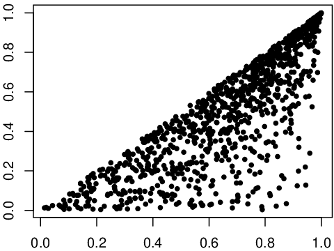
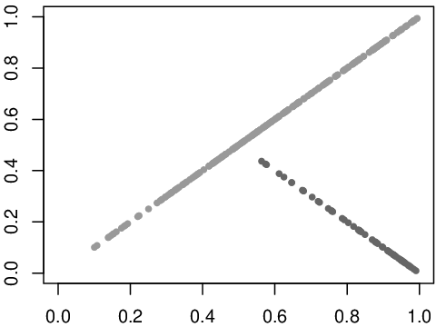
Let X2X_{2} be uniformly distributed on [0,1][0,1], and let X1X_{1} be distributed as the maximum of X2X_{2} and another independent uniformly distributed random variable, that is, F1​(x)=x2F_{1}(x)=x^{2}. In this case H⁡(s)=s−s2H(s)=s-s^{2} is unimodal with the maximum at r=1/2r=1/2, and t⁡(s)=1−st(s)=1-s for s∈(r,1]s\in(r,1]. The top-left panel of Fig. 1 shows a sample from the distribution LL. It is easily seen that these values belong to the set AA given by (8) which consists here of the diagonal of the square [0,1]2[0,1]^{2} and the lower part of the off-diagonal.
Refer to caption
Refer to caption
Refer to caption
Fig. 1: Top-left panel: Sample of size n=300n=300 of points (dark and light gray) from the maximally independent joint distribution LL for Example 7; Top-right panel: Histograms of two subsamples of a sample of LL of size n=50000n=50000 depending on whether the points are on the diagonal (light gray) or the off-diagonal (dark gray); Bottom panel: Sample of size n=1000n=1000 of points from the entropy maximizing distribution in Example 7.

The smallest values for Kendall’s tau and Spearman’s rho are 1/31/3 and 1/41/4, respectively. The joint density with the maximal entropy is given by

f⁡(x1,x2)=2​(1−x1)(1−x2)2,0≤x2≤x1≤1.f(x_{1},x_{2})=\frac{2(1-x_{1})}{(1-x_{2})^{2}},\quad 0\leq x_{2}\leq x_{1}\leq 1. (25)

A sample from this distribution is shown in the bottom panel of Fig. 1. Note that in this example it is easy to simulate from the distribution LL, and also from the distribution with density ff given at (25). To simulate a random vector (X1,X2)(X_{1},X_{2}) with distribution LL, generate a random variable UU which is uniformly distributed on [0,1][0,1] and set

(X1,X2)={(U,U),U≤1/4,((1+4​U−1)/2,(1−4​U−1)/2),1/4<U<1/2,(U,U),U≥1/2.(X_{1},X_{2})=\begin{cases}(\sqrt{U},\sqrt{U}),&U\leq 1/4,\\ ((1+\sqrt{4U-1})/2,(1-\sqrt{4U-1})/2),&1/4<U<1/2,\\ (U,U),&U\geq 1/2.\end{cases}

A random vector (X1,X2)(X_{1},X_{2}) with distribution given by the density ff at (25) is obtained by simulating independent random variables U,VU,V both uniformly distributed on [0,1][0,1] and defining

(X1,X2)=(1−V​(1−U),U).(X_{1},X_{2})=(1-\sqrt{V}(1-U),U).
Example 8.

Theorem 1 establishes a relationship between the distribution of (X1,X2)(X_{1},X_{2}) and the order statistics of a suitably chosen exchangeable pair (V1,V2)(V_{1},V_{2}). Assume that V1V_{1} and V2V_{2} are independent. Then ℙ⁡(V1≤x,V2≤x)=G​(x)2\mathbb{P}(V_{1}\leq x,V_{2}\leq x)=G(x)^{2}. By Theorem 1, F1​(x)=G​(x)2F_{1}(x)=G(x)^{2}, whence

F2​(x)=2​F1​(x)−F1​(x),x∈ℝ.F_{2}(x)=2\sqrt{F_{1}(x)}-F_{1}(x),\quad x\in\mathbb{R}.

Then

H⁡(x)=2​F1​(x)​(1−F1​(x))H(x)=2\sqrt{F_{1}(x)}(1-\sqrt{F_{1}(x)})

is always unimodal. If F1F_{1} is continuous the maximum attained at any lower quartile of X1X_{1}. The smallest possible Kendall’s tau equals −1/3-1/3; it does not depend on F1F_{1}. If we assume additionally that the support of F1F_{1} is an interval, Theorem 10 applies and the equation used to find t⁡(s)t(s) turns into F1​(t​(s))=1−F1​(s)\sqrt{F_{1}(t(s))}=1-\sqrt{F_{1}(s)}. Substituting this in (19) yields that Spearman’s rho equals −1/2-1/2 for all F1F_{1}. If F1F_{1} is absolutely continuous with density f1f_{1} the maximum entropy is attained on the density f⁡(x1,x2)=2​g​(x1)​g​(x2)f(x_{1},x_{2})=2g(x_{1})g(x_{2}), x1≥x2x_{1}\geq x_{2}, where g⁡(x)=f1​(x)/(2​F1​(x))g(x)=f_{1}(x)/(2\sqrt{F_{1}(x)}).

Example 9.

Let X1X_{1} be uniform on [0,1][0,1], and let X2=X11/αX_{2}=X_{1}^{1/\alpha} with α∈(0,1]\alpha\in(0,1]. Then F1​(x)=xF_{1}(x)=x, F2​(x)=xαF_{2}(x)=x^{\alpha}, and

F⁡(x1,x2)=2​C~​((x1+x1α)/2,(x2+x2α)/2)−x2F(x_{1},x_{2})=2\tilde{C}((x_{1}+x_{1}^{\alpha})/2,(x_{2}+x_{2}^{\alpha})/2)-x_{2}

for x1≥x2x_{1}\geq x_{2}, see (2). In this case, (9) yields that

L⁡(x1,x2)={x1,x1≤x2,x2α−min⁡{x2α−x2,x1α−x1},otherwise,L(x_{1},x_{2})=\begin{cases}x_{1},&x_{1}\leq x_{2},\\ x_{2}^{\alpha}-\min\{x_{2}^{\alpha}-x_{2},x_{1}^{\alpha}-x_{1}\},&\text{otherwise},\end{cases}

The function F2−F1F_{2}-F_{1} is unimodal and attains its maximum at r=α(1−α)−1r=\alpha^{(1-\alpha)^{-1}}. The smallest Kendall’s tau is

τ=3−4​𝔼​X1α=3​α−11+α.\tau=3-4\;\mathbb{E}X_{1}^{\alpha}=\frac{3\alpha-1}{1+\alpha}.

Note that τ=1\tau=1 if α=1\alpha=1, τ=0\tau=0 if α=1/3\alpha=1/3, and τ→−1\tau\to-1 as α↓0\alpha\downarrow 0.

We are not able to provide an explicit formula for Spearman’s rho in terms of α\alpha but Fig. 2 shows τ\tau and ρ\rho as a function of α\alpha.

Refer to caption
Fig. 2: Kendall’s tau τ\tau and Spearman’s rho ρ\rho as functions of α∈(0,1]\alpha\in(0,1] for the distributions in Example 9.
Example 10 (Unimodal densities).

Let ZZ be a random variable with cdf FF and unimodal density ff whose support is ℝ\mathbb{R}. Let Xi=Z+μiX_{i}=Z+\mu_{i}, i=1,2i=1,2, with μ1≥μ2\mu_{1}\geq\mu_{2}, hence Fi=F(⋅−μi)F_{i}=F(\cdot-\mu_{i}), i∈{1,2}i\in\{1,2\}. Then Theorem 9 yields for Kendall’s tau of the distribution LL at (9)

τ=3−4​𝔼​F​(Z+μ1−μ2)=4​∫Fˇ​(μ2−μ1−z)​𝑑F​(z)−1,\tau=3-4\;\mathbb{E}F(Z+\mu_{1}-\mu_{2})=4\int\check{F}(\mu_{2}-\mu_{1}-z)\,\mathrm{d}F(z)-1,

which is the convolution of Fˇ​(z):=1−F​(−z)\check{F}(z):=1-F(-z) and FF.

Let us additionally assume that ff is symmetric about its mode at zero. Then Fˇ=F\check{F}=F, and the unimodal function F2−F1F_{2}-F_{1} has its maximum at r=(μ1+μ2)/2r=(\mu_{1}+\mu_{2})/2. Hence, the function t:(r,∞)→(−∞,r)t:(r,\infty)\to(-\infty,r) in Theorem 10 is given by t⁡(s)=μ2+μ1−st(s)=\mu_{2}+\mu_{1}-s. If F=ΦF=\Phi is the standard Gaussian cdf, then Φ∗Φ⁡(x)=Φ⁡(x/2)\Phi*\Phi(x)=\Phi(x/\sqrt{2}), and, therefore,

τ=4​Φ​((μ2−μ1)/2)−1.\tau=4\Phi((\mu_{2}-\mu_{1})/\sqrt{2})-1.

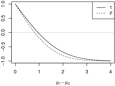
In particular, τ=1\tau=1 if μ1=μ2\mu_{1}=\mu_{2}, τ=0\tau=0 if μ1−μ2=2​Φ−1​(3/4)≈0.954\mu_{1}-\mu_{2}=\sqrt{2}\Phi^{-1}(3/4)\approx 0.954, and if μ1−μ2→∞\mu_{1}-\mu_{2}\to\infty, then τ→−1\tau\to-1.

For Spearman’s rho, we numerically computed the integrals in (19) for F=ΦF=\Phi. The values of τ\tau and ρ\rho as functions of μ1−μ2≥0\mu_{1}-\mu_{2}\geq 0 are displayed in Fig. 3.

Refer to caption
Fig. 3: Kendall’s tau τ\tau and Spearman’s rho ρ\rho as functions of μ1−μ2∈[0,4]\mu_{1}-\mu_{2}\in[0,4] for F=ΦF=\Phi in Example 10.
Example 11 (Exponential marginal distributions).

Let ZZ be an exponential random variable with cdf F⁡(x)=1−e−xF(x)=1-e^{-x}, and let Xi=Z/λiX_{i}=Z/\lambda_{i}, i∈{1,2}i\in\{1,2\}, with λ1≤λ2\lambda_{1}\leq\lambda_{2}. Considering log⁡(Xi)\log(X_{i}), i∈{1,2}i\in\{1,2\} shows that we are in the same setting as in Example 10 because Kendall’s tau and Spearman’s rho are invariant under monotone transformations of the marginals and the stochastic ordering is preserved if we transform both marginals with the same increasing function.

However, we can also compute τ\tau and ρ\rho directly. Kendall’s tau is given by

τ=4​∫01(1−u)λ2/λ1​𝑑u−1=3​λ1−λ2λ1+λ2.\tau=4\int_{0}^{1}(1-u)^{\lambda_{2}/\lambda_{1}}\,\mathrm{d}u-1=\frac{3\lambda_{1}-\lambda_{2}}{\lambda_{1}+\lambda_{2}}.

Note that τ=1\tau=1 if λ1=λ2\lambda_{1}=\lambda_{2}, τ=0\tau=0 if λ1/λ2=1/3\lambda_{1}/\lambda_{2}=1/3, and τ→−1\tau\to-1 as λ1/λ2↓0\lambda_{1}/\lambda_{2}\downarrow 0.

The function

F2​(x)−F1​(x)=F⁡(λ2​x)−F⁡(λ1​x)=e−λ1​x−e−λ2​xF_{2}(x)-F_{1}(x)=F(\lambda_{2}x)-F(\lambda_{1}x)=e^{-\lambda_{1}x}-e^{-\lambda_{2}x}

is unimodal on [0,∞)[0,\infty) with maximum at

r=(log⁡λ2−log⁡λ1)/(λ2−λ1).r=(\log\lambda_{2}-\log\lambda_{1})/(\lambda_{2}-\lambda_{1}).

Therefore, we can use (19) to compute ρ\rho. Considering the increasing transformation λ1​Xi\lambda_{1}X_{i}, i∈{1,2}i\in\{1,2\}, we see that τ\tau and ρ\rho only depend on λ1/λ2≤1\lambda_{1}/\lambda_{2}\leq 1. Fig. 4 provides plots of τ\tau and ρ\rho as functions of λ1/λ2∈(0,1]\lambda_{1}/\lambda_{2}\in(0,1].

Refer to caption
Fig. 4: Kendall’s tau τ\tau and Spearman’s rho ρ\rho in terms of λ1/λ2\lambda_{1}/\lambda_{2} for exponentially distributed marginal distributions as in Example 11.

7 Generalizations

A multivariate version of Theorem 1 is the following.

Theorem 12.

A random vector (X1,…,Xn)(X_{1},\dots,X_{n}) with marginal cdfs F1,…,FnF_{1},\dots,F_{n} satisfies ℙ⁡(X1≥⋯≥Xn)=1\mathbb{P}(X_{1}\geq\dots\geq X_{n})=1 if and only if Xi=V(i)X_{i}=V_{(i)} where V(1)≥⋯≥V(n)V_{(1)}\geq\dots\geq V_{(n)} are the order statistics of a random vector (V1,…,Vn)(V_{1},\dots,V_{n}) with exchangeable components and such that for j=1,…,nj=1,\dots,n

ℙ⁡(V1≤x,…,Vj≤x)=1(nj)​∑ℓ=1n−j+1(n−ℓj−1)​Fℓ​(x).\mathbb{P}(V_{1}\leq x,\dots,V_{j}\leq x)=\frac{1}{\binom{n}{j}}\sum_{\ell=1}^{n-j+1}\binom{n-\ell}{j-1}F_{\ell}(x).
Proof.

Let (V1,…,Vn)(V_{1},\dots,V_{n}) be an exchangeable random vector that satisfies the above condition. By [17, Proposition 4.4.1], we have that

ℙ⁡(V(i)≤x)\displaystyle\mathbb{P}(V_{(i)}\leq x) =∑j=n−i+1n(−1)j−(n−i+1)​(j−1n−i)​(nj)​ℙ​(V1≤x,…,Vj≤x)\displaystyle=\sum_{j=n-i+1}^{n}(-1)^{j-(n-i+1)}\binom{j-1}{n-i}\binom{n}{j}\mathbb{P}(V_{1}\leq x,\dots,V_{j}\leq x)
=∑j=n−i+1n(−1)j−(n−i+1)​(j−1n−i)​∑ℓ=1n−j+1(n−ℓj−1)​Fℓ​(x)\displaystyle=\sum_{j=n-i+1}^{n}(-1)^{j-(n-i+1)}\binom{j-1}{n-i}\sum_{\ell=1}^{n-j+1}\binom{n-\ell}{j-1}F_{\ell}(x)
=∑ℓ=1iFℓ​(x)​(n−ℓn−i)​∑j=n−i+1n−ℓ+1(−1)j−(n−i+1)​(i−ℓn−ℓ−j+1)\displaystyle=\sum_{\ell=1}^{i}F_{\ell}(x)\binom{n-\ell}{n-i}\sum_{j=n-i+1}^{n-\ell+1}(-1)^{j-(n-i+1)}\binom{i-\ell}{n-\ell-j+1}
=Fi​(x).\displaystyle=F_{i}(x).

Conversely, if the vector (V1,…,Vn)(V_{1},\dots,V_{n}) is obtained as the random permutation of (X1,…,Xn)(X_{1},\dots,X_{n}), then it is exchangeable and the formula for ℙ⁡(V1≤x,…,Vj≤x)\mathbb{P}(V_{1}\leq x,\dots,V_{j}\leq x) is essentially the inversion of the first equality in the above equation. ∎

A variant of Theorem 1 applies to random elements in a lattice EE with partial order ⪯\preceq, and with ∨\vee being the maximum and ∧\wedge being the minimum operation. Endow EE with the σ\sigma-algebra generated by {y:y⪯x}\{y:\;y\preceq x\} for all x∈Ex\in E. Since these events form a π\pi-system, the values ℙ⁡(X⪯x)\mathbb{P}(X\preceq x), x∈Ex\in E, uniquely determine the distribution of an EE-valued random element XX.

In this case, Theorem 1 admits a direct generalization. Namely X1⪯X2X_{1}\preceq X_{2} a.s. if and only if X1=V1∨V2X_{1}=V_{1}\vee V_{2} and X2=V1∧V2X_{2}=V_{1}\wedge V_{2} for a pair (V1,V2)(V_{1},V_{2}) of exchangeable random elements in EE such that

ℙ⁡(Vi⪯x)=12​(ℙ⁡(X1⪯x)+ℙ⁡(X2⪯x))\mathbb{P}(V_{i}\preceq x)=\frac{1}{2}\Big(\mathbb{P}(X_{1}\preceq x)+\mathbb{P}(X_{2}\preceq x)\Big)

and ℙ⁡(V1⪯x,V2⪯x)=ℙ⁡(X1⪯x)\mathbb{P}(V_{1}\preceq x,V_{2}\preceq x)=\mathbb{P}(X_{1}\preceq x).

Acknowledgement

The problem of characterizing bivariate copulas with stochastically ordered marginals was brought to the attention of the second author by Nicholas Kiefer from the Economics Department at Cornell University.

The authors are grateful to the referees for spotting mistakes in the original version of this paper and suggesting numerous improvements.

References

  • [1] J. Navarro, F. Spizzichino, On the relationships between copulas of order statistics and marginal distributions, Statist. Probab. Lett. 80 (2010) 473–479.
  • [2] R. Lebrun, A. Dutfoy, Copulas for order statistics with prescribed margins, J. Multivariate Anal. 128 (2014) 120–133.
  • [3] M. Dietz, S. Fuchs, K. D. Schmidt, On order statistics and their copulas, Statist. Probab. Lett. 117 (2016) 165–172.
  • [4] F. Durante, R. Mesiar, C. Sempi, Copulas with given diagonal section: some new results, in: Proc. of the Joint 4th Conf. of the European Society for Fuzzy Logic and Technology and the 11th Rencontres Francophones sur la Logique Floue et ses Applications, 2005, pp. 931–936.
  • [5] P. Embrechts, M. Hofert, A note on generalized inverses, Math. Method. Oper. Res. 77 (2013) 423–432.
  • [6] B. Schweizer, A. Sklar, Probabilistic Metric Spaces, North-Holland Publishing Co., New York, 1983.
  • [7] A. McNeil, J. Nešlehová, Multivariate archimedean copulas, dd-monotone functions and l1l_{1}-norm symmetric distributions, Ann. Stat. 37 (2009) 3059–3097.
  • [8] R. B. Nelsen, J. J. Quesada Molina, J. A. Rodríguez Lallena, M. Úbeda Flores, Best-possible bounds on sets of bivariate distribution functions, J. Multivariate Anal. 90 (2004) 348–358.
  • [9] E. P. Klement, A. Kolesárová, Extensions to copulas and quasi-copulas as special 1-Lipschitz aggregation operators, Kybernetika 41 (2005) 329–348.
  • [10] G. A. Fredricks, R. B. Nelsen, The Bertino family of copulas, in: C. M. Cuadras, J. Fortiana, J. A. Rodríguez-Lallena (Eds.), Distributions With Given Marginals and Statistical Modelling, Springer, Dordrecht, 2002.
  • [11] L. C. G. Rogers, Fastest coupling of random walks, J. London Math. Soc. (2) 60 (1999) 630–640.
  • [12] S. T. Rachev, L. Rüschendorf, Mass Transportation Problems. Vol. II, Springer-Verlag, New York, 1998.
  • [13] J. Nešlehová, On rank correlation measures for non-continuous random variables, J. Multivariate Anal. 98 (2007) 544–567.
  • [14] T. M. Cover, J. A. Thomas, Elements of Information Theory, 2nd Edition, Wiley-Interscience, Hoboken, NJ, 2006.
  • [15] C. Butucea, J.-F. Delmas, A. Dutfoy, R. Fischer, Maximum entropy distribution of order statistics with given marginals, Bernoulli 24 (2018) 115–155.
  • [16] C. Butucea, J.-F. Delmas, A. Dutfoy, R. Fischer, Maximum entropy copula with given diagonal section, J. Multivariate Anal. 137 (2015) 61–81.
  • [17] K. Lange, Applied Probability, Springer, New York, 2010.