Spin transparency for an interface of an ultrathin magnet within the spin dephasing length
Abstract
We examine a modified drift-diffusion formalism to describe spin transport near an ultrathin magnet whose thickness is similar to or less than the spin dephasing length. Most of the previous theories on spin torque assume the transverse component of a injected spin current dephases perfectly thus are fully absorbed into the ferromagnet. However, in the state-of-art multilayer systems under consideration of recent studies, the thicknesses of ferromagnets are on the order of or less than a nanometer, thus one cannot safely assume the spin dephasing to be perfect. To describe the effects of a finite dephasing rate, we adopt the concept of transmitted mixing conductance, whose application to the drift-diffusion formalism has been limited. For a concise description of physical consequences, we introduce an effective spin transparency. Interestingly, for an ultrathin magnet with a finite dephasing rate, the spin transparency can be even enhanced and there arises a non-negligible field-like spin-orbit torque even in the absence of the imaginary part of the spin mixing conductance. The effective spin transparency provides a simple extension of the drift-diffusion formalism, which is accessible to experimentalists analyzing their results.
pacs
I Introduction
Spin torque Slonczewski1996; Berger1996; Ralph2008 has been a central concept in magnetism for a few decades, as it allows electrical control of magnetism. When a spin current is injected to a ferromagnet, its transverse component to magnetization dephases rapidly, thus its angular momentum is transferred to the magnetization, giving rise to a torque Waintal2000; Heide2001; Zhang2002; Stiles2002. It is typically assumed that the spin dephasing in the ferromagnetic bulk is infinitely fast, thus the spin current right at the interface solely determines the total angular momentum transfer to the ferromagnet Shpiro2003. Indeed, the spin dephasing length is on the order of or less than a nanometer Zhang2004; Ghosh2012; Balaz2016, this assumption has provided a very simple but still reasonable way to calculate a spin torque.
Theoretically, the spin current at the interface is usually obtained by the drift-diffusion formalism Valet1993; Zhang2002; Shpiro2003 with imposing proper boundary conditions (BCs). Considering a ferromagnet much thicker than the spin dephasing length, as illustrated in Fig. 1(a), one may assume that the transverse component of an injected spin current at the interface 1 does not reach the interface 2. Hence, as far as transverse spin transport is concerned, the two interfaces do not communicate with each other. Therefore, in the normal metal side near an interface, the transverse spin current at the interface, say , is solely determined by the nonequilibrium spin chemical potential at the interface. Their relation is given by the celebrated magnetoelectronic circuit theory Brataas2000; Brataas2001; Brataas2006:
| (1) |
Here is the spin mixing conductance of the interface, is the electron charge, is the transverse spin current flowing to the normal metal side, is the nonequilibrium spin chemical potential in the normal metal side, and is the unit vector along magnetization in the magnetic layer. and are the coefficients for the Slonczewski-like torque [] Slonczewski1996 and the field-like torque () Xiao2008; Oh2009, respectively. With the BC [Eq. (I)], the spin drift-diffusion equation determines the spatial profiles of and self-consistently, and the spin torque to the ferromagnet is then calculated by the spin current right at the interface. The drift-diffusion formalism with the BC in Eq. (I) has been used for numerous theories Chen2013; Haney2013; Taniguchi2015; Amin2016; Amin2016a; Lee2013; Zhang2016 and experiments Nakayama2012; Feng2012; RojasSanchez2014; Zhang2015; Nguyen2016; Qiu2016.
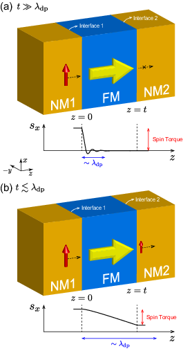
A relatively intuitive way to understand the self-consistent procedure is introducing the spin transparency Zhang2015 of a given interface.11 1 Here, we denoted the reported ‘transparency’ by the ‘spin transparency’, to emphasize that it is irrelevant for charge transport. For instance, the spin transparency is not necessarily zero for a magnetic insulator, through which a charge current cannot flow. Still, it is worth noting that the spin transparency considered throughout this paper is the one for the transverse spin transport, not the longitudinal one. The spin transparency determines how effectively a given perturbation generates a spin torque. More explicitly, denoting the spin transparency for the interface by and assuming a spin current injection , the resulting spin torque is determined by , not itself, because of the effects of spin diffusion in bulk and the reflection at boundaries. In this sense, the spin transparency can be understood by the absorption efficiency of a transverse spin current at the given interface. As one can expect, the spin transparency depends on the spin mixing conductance of the interface and the properties of the normal metal [see Eq. (10c) for an explicit expression]. Note that, for a trilayer system consisting of a thick film where the two interfaces hardly communicate with each other [Fig. 1(a)], the transparency at an interface is not affected by the properties of the normal metal at the other side.
However, recent interest of researches in magnetism has moved to ultrathin magnetic films, which not only allow high density spintronic applications but also result in much richer physics originating from broken symmetry such as spin-orbit torque (SOT) Miron2011; Liu2012, the Dzyaloshinskii-Moriya interaction Dzaloshinsky1958; Moriya1960; Fert1980, and other chiral phenomena Schulz2012; Kim2012; Kim2013; Je2013; Yin2016; Moon2013. The typical order of magnitudes of thicknesses of ferromagnetic layers under consideration is a few ÅMiron2011a; Liu2012a; Woo2016; Je2013; Emori2013; Ryu2013; Yin2016, which cannot be assumed to be sufficiently larger than the spin dephasing length. Moreover, there are recent experimental reports on a ferrimagnetic multilayer with an extremely long spin coherence length Yu2019 and a direct experimental evidence that the two interfaces of an ultrathin ferromagnet is no longer independent Qiu2016. Therefore, to correctly analyze the magnetic multilayers of contemporary research interest, it is desirable to construct a formal theory taking into account a finite dephasing rate of transverse spins and the resulting communication between the two interfaces of a magnetic layer.
For this purpose, it is necessary to examine the transport of a transverse spin current through a ferromagnetic layer. To do this, we adopt the concept of the transmitted mixing conductance suggested by previous works Qiu2016; Kovalev2006; Zwierzycki2005. As visualized in Fig. 2(a), the transmitted mixing conductance is the transmission counterpart of the conventional (reflected) spin mixing conductance (See Appendix A for mathematical details). Therefore, it is a suitable concept for describing the intercommunication of the two interfaces of the ferromagnetic layer. However, its application to the drift-diffusion formalism has been very limited (to our knowledge, only to Ref. Qiu2016). Even in the previous attempt, they consider a particular limit where physical insight is more easily obtained, but the general solution is too complicated to go beyond such a simple case. In this paper, we introduce an effective spin transparency, which provides a clear physical generalization of the conventional spin transparency, as well as significantly simplifies the complicated solution of the drift-diffusion equation in the general case. With the help of this general formalism, we demonstrate that the enhanced spin-orbit torque is realizable even without a special type of the interface Qiu2016 and that there arises a nonnegligible field-like spin-orbit torque even in the absence of the imaginary part of the spin mixing conductance. Thus, introducing the effective transparency in our formalism is a useful tool to study general consequences of spin transport near an ultrathin ferromagnet.
This paper is organized as follows. In Sec. II, we briefly review the conventional drift-diffusion formalism and present the modified BC for ultrathin films. In Sec. III, we solve the drift-diffusion equation and calculate various physical quantities such as SOT, the inverse spin Hall current, and the spin pumping effect. To express our result in simple forms, we introduce an effective spin transparency. In Sec. IV, we summarize the paper. Appendixes include mathematical information that is not crucial for the main flow of the paper.
II Formalism
II.1 Review of the conventional spin drift-diffusion formalism
In this section, we review the spin drift-diffusion formalism with the conventional BC for thick ferromagnetic film. We consider an arbitrary magnetic multilayer system. It is usually assumed that the mean free path is much shorter than the spin diffusion length Valet1993, then the spin chemical potential and the spin current in the normal metal bulk satisfy the spin drift-diffusion equation. Taking notations in Ref. Chen2013, the set of equations reads22 2 In this paper, the longitudinal part of the equation is ignored and it does not affect the calculation of spin torque and spin pumping at all.
| (2a) | |||
| where is the spin diffusion length for each normal metal layer and is the index of the layer. Since can be different for each layer, the nonequilibrium chemical potential is defined piecewisely. The spin current flowing along in the normal metal bulk is given by the drift-diffusion current: | |||
| (2b) | |||
| where is the electrical conductivity of the normal metal and is the electron charge. In Eq. (2b), one may introduce additional term if there is another current source. A famous example is the spin Hall current that we introduce in Sec. III.1. | |||
To obtain the full solution of and , one should apply proper BCs at each of the interfaces between two layers. The form of the BC depends on the type of the interface. Suppose that there is an interface at . (i) For an interface between a normal metal layer and the vacuum, should be satisfied. (ii) For an interface between two normal metal layers, is satisfied where is the interface conductance of the interface and is the spin chemical potential drop at the interface. (iii) For an interface between a normal metal and a ferromagnet, the BC is given by the circuit theory [Eq. (I)].
Now we explicitly apply this knowledge to the magnetic trilayer depicted in Fig. 1 and construct our model. The magnetic trilayer consists of a ferromagnetic layer (FM) sandwiched by two normal metal layers (NM1 and NM2): NM1()/FM()/NM2(), where and are the thicknesses of the normal metal layers and is the thickness of the ferromagnet. First of all, the equation in NM1 and NM2 is piecewisely given by Eq. (2) where we denote NM1 and NM2 by respectively. For the boundaries with the vacuum,
| (3) |
should be satisfied. For the BC at and (interfaces between normal metals and the ferromagnet),33 3 In Eq. (4a), the presence of the minus sign in front of is because .
| (4a) | ||||
| (4b) | ||||
where is the spin mixing conductance of each interface (), is a linear operator defined by for a three-dimensional vector , which allows compactly expressing the two terms in Eq. (I) by a single term. If there is time-varying magnetization, the spin pumping yields additional terms in the BC Tserkovnyak2002; Lee2013 as we consider in Sec. III.3.
To calculate the SOT per unit area, we use the angular momentum conservation. Note that is the incoming angular momentum to the ferromagnet and is the outgoing angular momentum from the ferromagnet. Therefore, the angular momentum absorbed by the ferromagnet is given by . Considering the conversion factor from the electrical current and the spin angular momentum, the SOT per unit area is given by
| (5) |
II.2 Modified BC by the transmitted mixing conductance
In this section, we modify the formalism in Sec. II.1 to take an ultrathin film into account. When the thickness of the magnet is not much larger than the spin dephasing length, the spin chemical potential at the interface 1 can generates the spin current at the interface 2 (and vice versa) [Fig. 1(b)]. In this case, it is necessary to introduce another conductance , called the transmitted mixing conductance Qiu2016 and whose properties are discussed below. As illustrated in the top part of Fig. 2(a), the transmitted mixing conductance connects and (and vice versa), giving the following modified BC.
| (6a) | ||||
| (6b) | ||||
Equation (6) gives a simple extension of the conventional BC [Eq. (4)] to allow for a finite dephasing rate. The formal derivation of Eq. (6) is presented in Appendix A.

There are three physical processes behind the transmitted mixing conductance [bottom part of Fig. 2(a)]. First, when a transverse spin is injected to and passing through the interface 1, there arise the interfacial spin filtering and the interfacial spin rotation, which make the spin current discontinuous at the interface . The details of the interfacial spin filtering and rotation are substantially discussed in Ref. Stiles2002. In Fig. 2(a), we denote this process by . The second process is the spin dephasing in the bulk of the magnetic layer. In this work, the spin dephasing is characterized by a thickness-dependent function , whose features for various materials are discussed below. The third process is the additional spin filtering and rotation at the interface 2 denoted by in Fig. 2(a). Now, we may write the transmitted mixing conductance by the following form.
| (7) |
where is the thickness of the magnet. is the interfacial contribution determined by and . is the bulk contribution and satisfies (no spin dephasing) and (perfect spin dephasing).
| Inside the magnetic layer, the transverse spin current decays rapidly over the spin dephasing length whose mechanisms determine the properties of . There are multiple origins of the spin dephasing; coherent and incoherent scatterings. For instance, in ferromagnetic metals, coherent spin oscillation of a number of electrons in the Fermi sea with different momenta is one of the main origins of the spin dephasing. In this case, is oscillatory and decaying approximately in the form of Stiles2002 | |||
| (8a) | |||
| where is the spin dephasing length, is the Fermi wave vector for spin , and is the spherical Bessel function: and . Indeed, this analytic form is valid for large limit (under the stationary phase approximation), but numerical calculations for Stiles2002; Zwierzycki2005 implies that this approximation works reasonably well in the aspect of qualitative understanding. For 3 transition metals, is on the order of a nanometer Zhang2004, thus is on the order of one for an ultrathin magnet. The physical interpretation of the oscillatory and decaying nature of is the precession of the incident spin around the magnetization, as illustrated in Fig. 2(b). In the case that there are incoherent scattering sources, an additional exponential factor can be introduced, but it results in quantitative corrections only. | |||
Although we focus on the ferromagnetic metal case [Eq. (8a)] in explicit numerical computations below, we discuss the form of for other systems as well. In most cases, an exponentially decaying is relevant. For example, in ferromagnetic insulators, the spin current is injected as magnon excitations, which decay over the spin-wave attenuation length or the magnon diffusion length Cornelissen2016. For systems with an extremely large coherence length Yu2019, the spin diffusion length would be the relevant length scale. For a magnet showing spin superfluidity Takei2014, the spin current decays algebraically rather than exponentially.
Two remarks are in order. First, although we only consider trilayers for writing Eq. (6), generalization of our theory to multilayer is straightforward. This is because normal metals are typically in the regime where the drift-diffusion equation is valid. Thus, one can write down the drift-diffusion equation in each layer and apply the modified BC [Eq. (6)] for all embedded magnetic layers. Second, consideration of the effects of interfacial spin-orbit coupling Amin2016; Amin2016a; Kim2017 goes beyond the scope of this paper. An additional consideration of the interface-generated spin current Amin2018 would be a way to generalize the formalism.
III Physical consequences
III.1 Transparency for injecting a spin Hall current

One of the most frequently performed experiments with ultrathin ferromagnets is injecting a spin Hall current to a ferromagnet to generate SOT Liu2012; Liu2012a; Zhang2015; Liu2011. Figure 3(a) shows the experimental situation under our consideration. When an electrical current is applied along the direction in NM1, the spin Hall effect Sinova2015 generates a torque to FM. The injection efficiency is determined by the spin transparency proposed in Ref. Zhang2015. As demonstrated in the previous paper and discussed in Sec. I, if the ferromagnet is thick enough, the two interfaces do not communicate with each other, thus the transparency of the interface 1 is solely determined by the properties of NM1 and the spin mixing conductance of the interface 1. However, if the spin dephasing is not perfect, the situation is no longer as simple as the previous result.
To calculate the spin Hall effect contribution, we add one more current source in NM1. The current in Eq. (2b) is modified as
| (9) |
where is the spin Hall conductivity of each normal metal, and is the applied electric field in NM1 along the direction.44 4 The spin Hall current contribution is absent in NM2 since no electric field is applied there. Consideration of an additional electric field applied in NM2 is very straightforward because the drift-diffusion equation is linear: calculating the consequences of electric field applied in each layer separately, and simply adding up the two results.
Now one can obtain the spatial profile of by solving Eqs. (2a) and (9) with the BCs in Eqs. (3) and Eq. (6). From the explicit solution available in Appendix B, one can use Eq. (5) to obtain the SOT per unit area:
| (10a) | ||||
| (10b) | ||||
| where is the effective spin transparency for the interface 1, is the normalized transmitted mixing conductance (dimensionless), is the conventional spin transparency for the interface , | ||||
| (10c) | ||||
| and the other transparency-like quantities are given by | ||||
| (10d) | ||||
| (10e) | ||||
The effective spin transparency is the central result of this paper. In the expression of , appears indirectly through . Note that Eq. (10b) restores the previously reported result Zhang2015 for where . For later purpose, we also define and by the same way as Eq. (10) except the exchange between subscripts and .
For simplicity of analysis, we assume that are positive real numbers and as considered in most experimental situations Zwierzycki2005. One can easily prove that is always smaller than (thus SOT cannot be enhanced) if is a positive real number. To mathematically show this, we use Eq. (10b) and verify that holds if and only if (See Appendix C for proof). In addition, it is also easy to show that if is positive and real (See Appendix D for proof). This gives , concluding the proof. Therefore, SOT is unlikely to be enhanced for a positive and real .
However, in more general cases that is not a positive real number, SOT can be enhanced. For metallic cases described by Eq. (8a), is on the same order of magnitude as , thus cannot be assumed to be positive and real. Furthermore, Eq. (8a) implies that can even be a negative real number, as also demonstrated in Refs. Zwierzycki2005; Kovalev2006; Balaz2016. For this case, , thus it is always smaller than . Thus SOT can be enhanced for a negative . More explicitly, we take Eq. (8a) for and plot as a function of in Fig 3(b). It clearly shows that, for some regions (), the spin torque can be enhanced () and there arises a nonnegligible field-like component of SOT () even for , which makes a qualitative difference from thick film cases.
The enhancement of spin torque can be understood by Fig. 1(b) Kovalev2006. For , Eq. (8a) has a negative real part, thus in Fig. 1(b) can be negative. Thus, the angular momentum transfer to the ferromagnet [] is larger than . A recent experiment Qiu2016 also suggests that the negativity of may enhance the SOT. In that experiment, the spin flip precisely at may result in being negative. This is an interfacial contribution ( in our convention), while the enhanced spin transparency in Fig. 3(b) originates from the bulk contribution () not requiring such a special interface.
III.2 Inverse spin Hall effect from NM2
One of physical consequences that are absent for but present for is the inverse spin Hall current in NM2. As depicted in Fig. 3(a), when an electric field is applied in NM1, the injected spin Hall current from NM1 can reach (blue) since the dephasing in the ferromagnetic bulk is not perfect. The nonzero spin current at may give rise to an inverse spin Hall current along in NM2 (green). To calculate the resulting charge current along , we assume that is perpendicular to the injected spin current since transport of a longitudinal spin in the ferromagnet is beyond the scope of this paper. The total inverse spin Hall current in NM2 is given by , where is the width of the wire and is the spin Hall angle, and is the spin Hall conductivity of NM2. Using the solution in Appendix B for , we obtain
| (11) |
In Fig. 4, We plot as a function of thickness with using the ansatz Eq. (8a). It changes the sign at , since the damping-like component of the transmitted spin changes its sign at this point. There are two remarks. First, from the expressions in Eq. (10), one can prove that Eq. (11) is symmetric under the exchange , as guaranteed by the Onsager reciprocity. Second, when an electric field is applied along NM1, a shunting current flowing through NM2 can affect the measurement of . To eliminate such contributions, one may use a charge insulator as the ferromagnet or an insertion layer.


III.3 Spin pumping
Spin pumping Tserkobnyak2005; Tserkovnyak2002 is another physical phenomenon in which the mixing conductances play an important role. It is frequently used for measuring the spin transparency Lee2018, the spin Hall angle RojasSanchez2014; Weiler2014; Wang2014, and the spin diffusion length Wang2014; Zhang2013. Here, we examine the effect of a nonzero on spin pumping for the geometry depicted in Fig. 5. In the presence of magnetization dynamics , angular momentum is pumped to both normal metals, as so-called the spin pumping currents (blue). These pumped currents generate measurable inverse spin Hall currents along the direction in each normal metal, which are denoted by (green). To calculate these currents, one needs to take into account the spin pumping currents as additional BCs. Taking the theory of spin pumping Tserkovnyak2002, we add
| (12a) | ||||
| (12b) | ||||
to Eqs. (6a) and Eq. (6b), respectively. Solving the same drift-diffusion equation [Eqs. (2a) and (9)] without the external electric field (), one obtains the spin current profile and the resulting inverse spin Hall currents in NM1 and NM2 given by . After some algebra,
| (13) |
The appearance of the same is understood by the Onsager reciprocity of spin pumping and spin torque. The factor is also understandable by Fig. 5 where the directions of the spin pumping currents to NM1 and NM2 are opposite. The inverse spin Hall measurement of the spin pumping effect can give separately.
However, the enhanced Gilbert damping Tserkovnyak2002 from the spin pumping effect requires more carefulness. This is because the Gilbert damping enhancement is not strictly given by the Onsager reciprocity when the system consists of multiple sources (interfaces 1 and 2) of angular momentum pumping. To calculate , we calculate the total angular momentum transfer per unit area as and project to to obtain its coefficient. Neglecting the renormalization of the gyromagnetic ratio Tserkovnyak2002, we obtain
| (14) |
where is the gyromagnetic ratio and is the saturation magnetization. Note that is given by the sum of for each interface with some weighting factors. Since the weighting factors [] for each interface are not identical, extracting from measurement of requires more experimental information.
IV Summary
In summary, we consider the effects of a nonzero transmitted mixing conductance in the drift-diffusion formalism to allow for the finite rate of the spin dephasing in an ultrathin ferromagnetic whose thickness is not much larger than the spin dephasing length. Solving the drift-diffusion equation with a modified BC, we demonstrate that spin torque can be enhanced in thin films, because of rotation of an injected spin current in ferromagnetic metals. Moreover, a nonnegligible field-like SOT can arise even in the absence of the imaginary part of the conventional spin mixing conductance. We demonstrate these by simply introducing an effective spin transparency, which also appears in the expression of the spin pumping current and the resulting Gilbert damping enhancement. The effective spin transparency obtained here provides a simple and straightforward extension of the conventional BC of the drift-diffusion formalism.
Acknowledgements.
The author acknowledges B. C. Min and O. J. Lee for motivating this work, D. S. Han for discussions, and K. J. Lee for critical reading of the manuscript. This work was financially supported by the KIST Institutional Program, the National Research Council of Science & Technology (NST) (Grant No. CAP-16-01-KIST), and the German Research Foundation (DFG) (No. SI 1720/2-1).Appendix A Derivation of the transmitted mixing conductance
To derive Eq. (6), it is required to extend the circuit theory Brataas2000; Brataas2001 to multiple interfaces. This is done in Sec 7.1 of Ref. Brataas2006. According to the theory, the current in NM1 side reads
| (15) |
where and are the transmission and reflection matrices for the transverse mode [denoted by ] incident from NM1 () and is the matrix in the Pauli spin space. The scattering matrices are defined by the scattering process over the entire ferromagnet consisting of two interfaces and bulk (not a single interface) (see Fig. 1 of Ref. Tserkovnyak2002 for a similar example). Compared to Ref. Brataas2006, an additional minus sign appears in our notation, since it is the current to the direction. Disregarding the charge degree of freedom, the relations between and in our theory are given by and where is the Pauli matrix. Following the procedure in Ref. Brataas2001, we disregard the spin-flip process in the contacts and write down the reflection and transmission matrices as
| (16) |
where is the spin-projection matrix. In this regime, the current matrix can be expressed in terms of , , , and . Then, the current is proportional to the transverse component of .
After some algebra, we obtain
| (17) |
where corresponds to the longitudinal transport, corresponds to the conventional mixing conductance, and corresponds to the transmitted mixing conductance (See Fig. 2). Here is the number of transverse modes. Taking only transverse part [second term in Eq. (17)] with introducing a proportionality constant connecting and gives Eq. (6a).
Appendix B Explicit solution of the spin drift-diffusion equation for spin Hall injection
Appendix C Condition for for a real
Provided that all the mixing conductances are real, all transparencies defined in Eq. (10) are real. We first look at the denominator of
| (19) |
Note that we assume and (see Appendix D), we obtain
| (20) |
implying that that the denominator is positive.
Then we look at the numerator. By noting that
| (21) |
Thus the numerator is also positive and .
Now we calculate
| (22) |
Since is positive, if and only if . Since the numerator is positive, the sign of is determined by that of . Hence, we conclude that
| (23) |
under our assumptions.
Appendix D Proof of for a positive real
First we define
| (24) |
then . Since and are positive, Eq. (24) implies that if is positive and real. Therefore, we obtain .
Next we consider
| (25) |
if is positive and smaller thatn . As a result, we obtain
References
- (1) J. C. Slonczewski, J. Magn. Magn. Mater. 159, L1 (1996).
- (2) L. Berger, Phys. Rev. B 54, 9353 (1996).
- (3) D. C. Ralph and M. D. Stiles, J. Magn. Magn. Mater. 320, 1190 (2008).
- (4) X. Waintal, E. B. Myers, P. W. Brouwer, and D. C. Ralph, Phys. Rev. B 62, 12317 (2000).
- (5) C. Heide, Phys. Rev. Lett. 87, 197201 (2001).
- (6) S. Zhang, P. M. Levy, and A. Fert, Phys. Rev. Lett. 88, 236601 (2002).
- (7) M. D. Stiles and A. Zangwill, Phys. Rev. B 66, 014407 (2002).
- (8) A. Shpiro, P. M. Levy, and S. Zhang, Phys. Rev. B 67, 104430 (2003).
- (9) J. Zhang, P. M. Levy, S. Zhang, and V. Antropov, Phys. Rev. Lett. 93, 256602 (2004).
- (10) A. Ghosh, S. Auffret, U. Ebels, and W. E. Bailey, Phys. Rev. Lett. 109, 127202 (2012).
- (11) P. Baláž, M. Zwierzycki, J.-P. Ansermet, and J. Barnaś, Phys. Rev. B 94, 144414 (2016).
- (12) T. Valet and A. Fert, Phys. Rev. B 48, 7099 (1993).
- (13) A. Brataas, Y. V. Nazarov, and G. E. W. Bauer, Phys. Rev. Lett. 84, 2481 (2000).
- (14) A. Brataas, Y. V. Nazarov, and G. E. W. Bauer, Eur. Phys. J. B 22, 99 (2001).
- (15) A. Brataas, G. E. W. Bauer, and P. J. Kelly, Phys. Rep. 427, 157 (2006).
- (16) J. Xiao, G. E. W. Bauer, and A. Brataas, Phys. Rev. B 77, 224419 (2008).
- (17) S.-C Oh, S.-Y. Park, A. Manchon, M. Chshiev, J.-H. Han, H.-W. Lee, J.-E. Lee, K.-T. Nam, Y. Jo, Y.-C. Kong, B. Dieny, and K.-J. Lee, Nature Phys. 5, 898 (2009).
- (18) Y.-T. Chen, S. Takahashi, H. Nakayama, M. Althammer, S. T. B. Goennenwein, E. Saitoh, and G. E. W. Bauer, Phys. Rev. B 87, 144411 (2013).
- (19) P. M. Haney, H.-W. Lee, K.-J. Lee, A. Manchon, and M. D. Stiles, Phys. Rev. B 87, 174411 (2013).
- (20) T. Taniguchi, J. Grollier, and M. D. Stiles, Phys. Rev. Applied 3, 044001 (2015).
- (21) V. P. Amin and M. D. Stiles, Phys. Rev. B 94, 104419 (2016).
- (22) V. P. Amin and M. D. Stiles, Phys. Rev. B 94, 104420 (2016).
- (23) K.-J. Lee, M. D. Stiles, H.-W. Lee, J.-H. Moon, K.-W. kim, and S.-W. Lee, Phys. Rep. 531, 89 (2013).
- (24) S. S.-L. Zhang and G. Vignale, Phys. Rev. B 94, 140411(R) (2016).
- (25) H. Nakayama, K. Ando, K. Harii, T. Yoshino, R. Takahashi, Y. Kajiwara, K. Uchida, Y. Fujikawa, and E. Saitoh, Phys. Rev. B 85, 144408 (2012).
- (26) Z. Feng, J. Hu, L. Sun, B. You, D. Wu, J. Du, W. Zhang, A. Hu, Y. Yang, D. M. Tang, B. S. Zhang, and H. F. Ding, Phys. Rev. B 85, 214423 (2012).
- (27) J.-C. Rojas-Sánchez, N. Reyren, P. Laczkowski, W. Savero, J.-P. Attané, C. Deranlot, M. Jamet, J.-M. George, L. Vila, and H. Jaffrés, Phys. Rev. Lett. 112, 106602 (2014).
- (28) W. Zhang, W. Han, X. Jiang, S.-H. Yang, and S. S. P. Parkin, Nature Phys. 11, 496 (2015).
- (29) M.-H. Nguyen, D. C. Ralph, and R. A. Buhrman, Phys. Rev. Lett. 116, 126601 (2016).
- (30) X. Qiu, W. Legrand, P. He, Y. Wu, J. Yu, R. Ramaswamy, A. Manchon, and H. Yang, Phys. Rev. Lett. 117, 217206 (2016).
- (31) I. M. Miron, K. Garello, G. Gaudin, P.-J. Zermatten, M. V. Costache, S. Auffret, S. Bandiera, B. Rodmacq, A. Schuhl, and P. Gambardella, Nature (London) 476, 189 (2011).
- (32) L. Liu, C.-F. Pai, Y. Li, H. W. Tseng, D. C. Ralph, and R. A. Buhrman, Science 336, 555 (2012).
- (33) I. J. Dzyaloshinsky, Phys. Chem. Solids 4, 241 (1958).
- (34) T. Moriya, Phys. Rev. 120, 91 (1960).
- (35) A. Fert and P. M. Levy, Phys. Rev. Lett. 44, 1538 (1980).
- (36) T. Schulz, R. Ritz, A. Bauer, M. Halder, M. Wagner, C. Franz, C. Pfleiderer, K. Everschor, M. Garst and A. Rosch, Nature Phys. 8, 301 (2012).
- (37) K.-W. Kim, J.-H. Moon, K.-J. Lee, and H.-W. Lee, Phys. Rev. Lett. 108, 217202 (2012).
- (38) K.-W. Kim, H.-W. Lee, K.-J. Lee, and M. D. Stiles, Phys. Rev. Lett. 111 216601 (2013).
- (39) S.-G. Je, D.-H. Kim, S.-C. Yoo, B.-C. Min, K.-J. Lee, and S.-B. Choe, Phys. Rev. B 88, 214401 (2013).
- (40) Yuxiang Yin, D.-S. Han, J.-. Kim, R. Lavrijsen, K.-J. Lee, S.-W. Lee, K.-W. Kim, H.-W. Lee, H. J. M. Swagten, and B. Koopmans, Appl. Phys. Lett. 110, 122401 (2016).
- (41) J.-H. Moon, S.-M. Seo, K.-J. Lee, K.-W. Kim, J. Ryu, H.-W. Lee, R. D. McMichael, and M. D. Stiles, Phys. Rev. B 88, 184404 (2013).
- (42) I. M. Miron, T. Moore, H. Szambolics, L. D. Buda-Prejbeanu, S. Auffret, B. Rodmacq, S. Pizzini, J. Vogel, M. Bonfim, A. Schuhl, and G. Gaudin, Nature Mater. 10, 419 (2011).
- (43) L. Liu, O. J. Lee, T. J. Gudmundsen, D. C. Ralph, and R. A. Buhrman, Phys. Rev. Lett. 109, 096602 (2012).
- (44) S. Woo, K. Litzius, B. Krüger, M.-Y. Im, L. Caretta, K. Richter, M. Mann, A. Krone, R. M. Reeve, M. Weigand, P. Agrawal, I. Lemesh, M.-A. Mawass, P. Fischer, M. Kläui, and G. S. D. Beach, Nature Mater. 15, 501 (2016).
- (45) S. Emori, U. Bauer, S.-M. Ahn, E. Martinez, and G. S. D. Beach, Nature Mater. 12, 611 (2013).
- (46) K.-S. Ryu, L. Thomas, S.-H. Yang, and S. S. P. Parkin, Nature Nanotechnol. 8, 527 (2013).
- (47) J. Yu, D. Bang, R. Mishra, R. Ramaswamy, J. H. Oh, H.-J. Park, Y. Jeong, P. Van Thach, D.-K. Lee, G. Go, S.-W. Lee, Y. Wang, S. Shi, X. Qiu, H. Awano, K.-J. Lee, and H. Yang, Nature Mater. 18, 29 (2019).
- (48) A. A. Kovalev, G. E. W. Bauer, and A. Brataas, Phys. Rev. B 73, 054407 (2006).
- (49) M. Zwierzycki, Y. Tserkovnyak, P. J. Kelly, A. Brataas, and G. E. W. Bauer, Phys. Rev. B 71, 064420 (2005).
- (50) Y. Tserkovnyak, A. Brataas, and G. E. W. Bauer, Phys. Rev. Lett. 88, 117601 (2002).
- (51) L. J. Cornelissen, K. J. H. Peters, G. E. W. Bauer, R. A. Duine, and B. J. van Wees, Phys. Rev. B 94, 014412 (2016).
- (52) S. Takei and Y. Tserkovnyak, Phys. Rev. Lett. 112, 227201 (2014).
- (53) K.-W. Kim, K.-J. Lee, J. Sinova, H.-W. Lee, and M. D. Stiles, Phys. Rev. B 96, 104438 (2017).
- (54) V. P. Amin, J. Zemen, and M. D. Stiles, Phys. Rev. Lett. 121, 136805 (2018).
- (55) L. Liu, T. Moriyama, D. C. Ralph, and R. A. Buhrman, Phys. Rev. Lett. 106, 036601 (2011).
- (56) J. Sinova, S. O. Valenzuela, J. Wunderlich, C. H. Back, and T. Jungwirth, Rev. Mod. Phys. 87, 1213 (2015).
- (57) Y. Tserkovnyak, A. Brataas, G. E. W. Bauer, and B. I. Halperin, Rev. Mod. Phys. 77, 1375 (2005).
- (58) D. J. Lee, J. H. Kim, H. G. Park, K.-J. Lee, B.-K. Ju, H.-C. Koo, B.-C. Min, and O. J. Lee, Phys. Rev. Appl. 10, 024029 (2018).
- (59) M. Weiler, J. M. Shaw, H. T. Nembach, and T. J. Silva, Phys. Rev. Lett. 113, 157204 (2014).
- (60) H. L. Wang, C. H. Du, Y. Pu, R. Adur, P. C. Hammel, and F. Y. Yang, Phys. Rev. Lett. 112, 197201 (2014).
- (61) W. Zhang, V. Vlaminck, J. E. Pearson, R. Divan, S. D. Bader, and A. Hoffmann, Appl. Phys. Lett. 103, 242414 (2013).
- (62) K. M. D. Hals, A. Brataas, and Y. Tserkovnyak, Europhys. Lett. 90, 47002, (2010).