Influence of static disorder and polaronic band formation on interfacial electron transfer in organic photovoltaic devices
Abstract
Understanding the interfacial charge-separation mechanism in organic photovoltaics requires, due to its high level of complexity, bridging between chemistry and physics. To elucidate the charge separation mechanism, we present a fully quantum dynamical simulation of a generic one-dimensional Hamiltonian, which physical parameters model prototypical PCBM or acceptor systems. We then provide microscopic evidence of the influence random static and dynamic potentials have on the interfacial charge-injection rate. In particular, we unveil that dynamic potentials, due to strong electron-vibration interactions, can lead to the formation of polaronic bands. Such dynamical potentials, when compared to random static potentials, can provide the main detrimental influence on the efficiency of the process of interfacial charge-separation.
I Introduction
Organic photovoltaic devices have currently attracted intense interest due to the potentially cheap production and their ability to environmentally friendly power generation li2012polymer; gunes2007conjugated; lu2015recent. The efficiency of these organic photovoltaic devices (OPVs) strongly depends on the charge separation process between materials that transport electrons (usually a fullerene derivative) or holes (usually a polymer). The energy offset caused by this interface drives electrons from the donor to the acceptor, while leaving holes left behind. Once the charges are in separate phases, they need to overcome their mutual Coulomb attraction. This binding energy is in the range of zhu2009charge; drori2008below; hallermann2008charge, which is much larger than the thermal energy of about at room temperature. Surprisingly, the charge separation process and eventually the formation of free charges that can be extracted at the electrodes is still very efficient shirakawa1977synthesis; morel1978high. In particular, experimental studies have shown, that the charge separation occurs on ultra-fast time scales in the range grancini2013hot; jailaubekov2013hot; gelinas2013ultrafast. At present, the mechanism responsible for charge separation is not well understood and still actively debated.
An obvious question in organic materials relates to the relative importance of static and dynamic potentials and their effect on the charge separation process. The static (time-independent) potential reflects the electron-hole Coulomb interaction, and the spatial disorder caused by electrostatic interactions resulting from the different environment in which each molecule is placed. This is particularly true for organic devices made up of two different disordered materials ballantyne2010understanding; hoppe2004organic where the spatial disorder is usually originating from the rather large permanent electric dipole of PCBM. However, we stress here, that contrary to PCBM, molecular dynamic simulations have shown, that , which has no permanent dipole, exhibits extremely limited disorder which thus can to a good extent be neglected d2016charges; tummala2015static. On the contrary, the dynamic potential is related to electron-vibration interactions that result in a time-dependent variation of microscopic transport parameters. Though debated gao2014charge; de2017vibronic, there are indications that, for charge separation, this effect could contribute falke2014coherent; song2014vibrational. Thus, the consideration of static and dynamic potentials seems unavoidable for a fully microscopic understanding of the charge separation mechanism in OPV devices. However, such microscopic descriptions are computationally challenging. To tackle these challenges, various numerical methods such as exact diagonalization wellein1997polaron; wellein1998self, diagrammatic Monte Carlo (DMC) de1983numerical; kornilovitch1998continuous, time-dependent density functional theory (TTDFT) rozzi2013quantum, and other approaches jeckelmann1998density; barivsic2002variational have been proposed. However, these methods are either quite expensive from a computational point of view or their application to non-translationally invariant systems remains unclear.
To overcome these difficulties the inhomogeneous version of the dynamical mean-field theory approximation (I-DMFT) potthoff1999surface; potthoff1999metallic; potthoff1999dynamical; delange2016large; backes2016hubbard; jacob2010dynamical; turkowski2012dynamical, a powerful non-perturbative technique for strongly interacting systems, has been introduced. By applying the I-DMFT approximation to a generic one-dimensional model Hamiltonian, which parameters model prototypical PCBM and based acceptor systems, we provide a fully quantum dynamical simulation of the charge separation process taking static (disorder + electron-hole Coulomb interaction) and dynamic potentials (electron-vibration interaction) into consideration. This provides the possibility to compute the charge injection rate at the donor-acceptor interface. Our work provides a step forward to a long-standing challenge in OPV, thereby bridging between chemistry and physics. In particular we unveil here, that dynamic potentials (related to polaron formation), when compared to random static potentials, present the main detrimental lose mechanism in OPVs devices. Yet it can in some instances lead to an enhancement of the charge transfer process.
This paper is organized as follows. Section II is divided into two parts: (A) we introduce the generic one-dimensional Holstein based Hamiltonian to model the charge carrier dynamics across organic model interfaces (B) we briefly introduce the used I-DMFT approximation and comment on its general numerical aspects. In section III we apply the I-DMFT approximation to study the charge carrier dynamics across donor-acceptor model interfaces. Finally, we provide a brief conclusion and outlook in section IV.
II Methodology
Inspired on the Holstein model used in bera2015impact, we use the following generic one-dimensional Hamiltonian to describe the microscopic charge transfer process of an electron at the molecular donor-acceptor interface:
| (1) | |||||
where () is the creation (destruction) operator of electrons, () is the creation (destruction) operator of phonons, is the relevant phonon frequency ( throughout this work), is the electron-phonon coupling strength, is the tunneling amplitude between the LUMO of the donor (site i = 0) and the first site of the LUMO of the acceptor, determines the Coulomb potential, is the electron hopping parameter, is the energy of the incoming electron and is the energy level of a molecule on the acceptor site which is taken to be a random variable (with a mean and a standard derivation ) drawn from a rectangular distribution. In this model, the static potential is given explicitly by the distribution of the onsite energies and the Coulomb potential between the electron and hole, while the dynamic potential is caused by the electron-phonon coupling term .
At this point, we want to note, that we make the following assumptions. First, we do not model the hole dynamics since the effects of hole diffusion usually lead to a reduction of the Coulomb interaction only resulting in an increase of the electron-hole separation yield athanasopoulos2017efficient; aram2016charge and since hole transfer typically occurs on time scales in the range which is several orders of magnitude slower than electron transfer long2014asymmetry. Second, we use a one-dimensional model to describe a complex three dimensional bulk molecular heterostructure, since the main features of the Holstein polaron do not depend strongly on the dimensionality of the system ku2002dimensionality and since we expect, that a realistic, three-dimensional nature of the system will lead to mainly quantitative changes in the quantum efficiency. Third, we assume a single high-frequency intramolecular mode of vibration (order of , i.e. a period of roughly ) only, although the involvement of multiple phonon modes provides additional transfer channels. However, in this work, we are interested in electron dynamics that concern the fast electron unbinding from the Coulomb well which occurs on time scales of . Therefore, the impact of weakly coupled low-frequency modes of vibration (order of , i.e. a period of roughly ) can be neglected, since final equilibration occurs at longer relaxation times xie2015full. Fourth, all computations are presented at zero temperature taking no entropic effects into consideration, since electronic and vibrational energy scales are much larger than , where is Boltzmann’s constant and is the temperature pelzer2016charge, and since we expect that a change in entropy plays a diminished role in the charge separation process in one-dimensional systems gregg2011entropy. The driving force for the charge separation mechanism is thus entirely of quantum mechanical nature steaming from the coupling of an initially discrete state (electron at the interface) to a final state in the continuum (electron on the acceptor side surrounded by a cloud of phonon excitations). Fifth, we note that in absence of electron-phonon interaction scattering on defects can lead to Anderson localization anderson1958absence and it will hinder electron transfer across the interface. Since it is well known, that in the case of one-dimensional infinite disordered systems, any amount of disorder produces Anderson localization, we have embedded the system into an effective medium which has been computed using the coherent potential approximation (CPA). The absence of Anderson localization within CPA Haydock_1974 will then mimic a system without localization at moderate disorder (except very close to the band-edges) throughout this work.
The approach that we propose is the use of the single-polaron I-DMFT approximation. The aim of I-DMFT is to fully address the relevant spatial variations of the physical properties, but still affording a good description of the physical processes of interest. A crucial aspect of I-DMFT is that it provides an interpolation between the non-interacting case, in which it gives the exact solution of the problem and the strong coupling limit in which is also becomes exact. In I-DMFT the local Green’s function is for one given realization of disorder and is defined as:
| (2) |
where , are hybridization function, respectively self-energy at site i and with being an infinitesimal small number. In standard I-DMFT procedures a self-consistent solutions is obtained iteratively at each z where one needs to compute repeatedly the diagonal of the inverse of a complex matrix, which dimension equals the number of lattice sites. Using conventional linear-algebra algorithms, this problem grows cubic with the size of the system freericks2016generalized.
We use an alternative approach to solve the I-DMFT self-consistency equations which is based on Haydock’s recursion scheme applied to suitably defined Hamiltonians and, in particular, which does not require the inverse of a complex matrix. Instead the Hamiltonian (1) is solved on the full lattice under the approximation that the electron-phonon self-energy is local depending on the frequency of the local phonon only. Self-consistency equations are than expressed in Hilbert-space such that the recursion technique by Haydock haydock1980solid can be used which makes this method immediately generalizable to any lattice geometry and/or disorder distribution while easily handling inhomogeneous systems of up to lattice sites in less than (sequential computation on an Intel Xeon E5-2670 processor).


An detailed explanation of the used I-DMFT approach can be found in the original work by richler2018inhomogeneous.
Finally, let us comment on general numerical aspects of the proposed I-DMFT formalism. The number of possible phonon configurations is infinite, but can be restricted to a finite, sufficiently large number in actual calculations by choosing , where is the maximum number of phonon excitations per site. Further, we simulate only a finite part of the total size of the system (). We then embedded the leftmost site into an effective medium which has been computed using the coherent potential approximation (CPA). We thus define a number of non-equivalent lattice sites along the surface. Choosing , and ensures that all results are independent of any system size characteristics, while keeping modest computational complexity. A pictorial representation of the proposed model is depicted in Fig. 1.
III Results
In the following we express all energies in units of (energy unit in and time unit in ) and take , , , and while keeping and as independent parameters. All are chosen such, that they are in a realistic experimental range to model the prototypical PCMB () and () acceptor systems zheng2017charge; d2016electrostatic; antropov1993phonons; faber2011electron; castet2014charge. We have checked that all results are qualitatively insensitive to different disorder configurations, a result that has been found in all tested cases throughout this work. Finally we note, that throughout this paper our initial state at time will consist of an electron at site having energy and no phonon modes excited, i.e. with being the vacuum state for phonons and electrons.
First, we present in Fig. 2 the probability density of the wave-function on the acceptor
| (3) |
where is the orthonormal basis vector of the -dimensional Krylov-space () gutknecht2007brief. The Krylov-states , which are computed by a Lanczos-based recursion method haydock1980solid, represent a basis of excitations of the many-body system (electron and phonon modes) that progressively spread away from the interface into the acceptor. The time evolution of the wave function in Krylov space is then defined as with being the reduced Hamiltonian of the Krylov subspace . The time-evolution has then been determined by an exact diagonalization technique by choosing the first Krylov-space vector equal to the initial state, i.e. (see Appendix A for a brief introduction to the Krylov subspace method and computation of wave-function ). This provides an efficient way to extract the essential character of the Hamiltonian (1) while using a limited number of basis sets. We stress here, that the size of the system (2000 states in the Krylov-space) is sufficient to prevent the wave packet to bounce back at the boundary.
We find, in the limit of sole dynamic potentials (, ) shown in Fig. 2(a), that the probability weight near the interface is progressively decaying with time and the particle is fully delocalized. Upon increasing the electron-phonon interaction (, ), the local density of states (LDOS) fragments into polaronic sub-bands (self-trapping) and where the strongly renormalized width of the polaronic sub-bands arises as the new energy scale ciuchi1997dynamical. As can be seen in Fig. 2(b) self-trapping of the electron hinders, in this case, the interfacial electron transfer drastically as parts of the wave-function remain localized at the interface resulting in a poor but finite interfacial charge-transfer efficiency. In panel (c), (d) of Fig. 2 we now present the combined effect of static spatial disorder and weak (, ), respectively strong (, ) dynamic potentials. As can be seen, the in panel (c), (d) presented physical picture does not change quantitatively when compared to panel (a), respectively (b), an outcome we have found throughout this work.
Before proceeding we stress here, that the LDOS is a key factor since its shape and, in particular, the energy distribution of electronic states are found to determine the value of practically achievable injection energies. This comes in handy when using the proposed formalism richler2018inhomogeneous. In particular, we have found, that taking the incoming electron energy outside the band of delocalized states completely suppresses, as expected, interfacial charge transfer (electron becomes localized at interface) while an incoming electron energy that is taken in the band of delocalized states results in interfacial charge transfer.

By making use of the by I-DMFT computed Green’s function and by applying Fermi’s Golden rule we now quantify, as a function of the incoming electron energy , the quantum mechanical donor-acceptor interface transfer rate
| (4) |
where is the imaginary part of the Green’s function . This present a simple measure of the efficiency for charge transfer at the donor-acceptor interface, but note, the transfer rate is related, but not equal to the internal quantum efficiency which is commonly extracted from experiments. The interface transfer rate is graphically depicted in Fig. 3 for incoming electron energies of , where this restriction is sufficient to assure the applicability of Eq. (4) (weak coupling to a quasi-continuum of states). Although, we do not model the competing electron-hole and/or geminate recombination processes, we have indicated in the same figure the range of experimentally observed recombination rate of order grancini2013hot; jailaubekov2013hot; gelinas2013ultrafast. Therefore, efficient charge transfer from the donor to the acceptor occurs when the interface transfer rate is large compared to the competing process of charge recombination . We start considering the case of sole, but weak dynamic potentials only (, ). We find, that the interfacial transfer rate is essentially, with the exception of values of close to the low energy edge, higher than the upper experimental recombination rate for all negative values of . On the contrary, this changes drastically for all positive values of , where interfacial charge transfer is large only, when compared to extremely low experimental ranges of recombination rates. This stems from strong relaxation processes (phonon emission) caused by molecular vibrations which are facilitated at higher energies. Upon increasing the electron-phonon interaction () multiple gaps throughout the spectrum arise and thus multiple values of occur that are below the experimental value of . This is readily explained since upon increasing the electron-phonon interaction the LDOS fragments into sub-bands that are separated by multiples of . This effect will drastically hinder the range of suitable incoming electron energies, since the incoming electron energy must be identical to that of the allowed unoccupied state of the acceptor material. Surprisingly, this picture does not change qualitatively when considering the combined effect of static disorder and dynamic potentials. In particular, we have found that weak but static disorder does not change drastically the interfacial transfer rate for incoming electron energies of . Finally, we note that these results are in agreement with the analysis of the time-evolution of the electron density shown above.
We note here, that we confine our analysis about the interfacial transfer rate by choosing realistic experimental values for all parameters. However, introducing , enables the scale transformation of the interfacial transfer rate into
| (5) |
where , are the scaling constants of , respectively. Through this scale transformation the results presented in Fig. 3 can then be adapted to describe physically equivalent systems having a different scale and set of parameters ().
Finally, we remark the following: First, we have not found interfacial electron-transfer in the limit of extremely strong electron-phonon coupling (). This is readily explained since in this limit the coupling between the donor and the first site of the acceptor becomes much larger than the renormalized bandwidth of the polaronic sub-bands. Thus, one is, to a good extent, left with two eigenstates separated by a larger energy offset giving rise to charge localization at the interface.
Second, we note that the results of our time-dependent study present some similarity with the Dirac-Frenkel time-dependent simulations in one-dimension bera2015impact where their study has focused on the interplay between electron-vibration interaction and the interfacial Coulomb interaction between the hole and electron. Yet, bera2015impact has not taken spatial disorder into consideration and has focused on the quantum yield in absence of any electron-hole recombination. The quantum yield, in absence of recombination, then simply measures the charge injected at infinite distance from the interface, i.e. their quantum yield is simply with being the weight of the wave-function localized near the interface. Instead, our study quantifies the charge injection-rate which is of more fundamental relevance since this quantity can be compared to the experimentally observed recombination rate. The quantum yield, in the presence of recombination, can then be obtained by
| (6) |
A high quantum yield is then given when holds. Moreover, the applicability of the in Ref. bera2015impact presented simulation is limited since their approximated treatment of the many-body nature of the polaronic state (momentum average approximation) is valid in the small bandwidth limit only. Contrary to Ref.bera2015impact, the proposed I-DMFT approach is accurate over the entire parameter space richler2018inhomogeneous.
IV Conclusion
To summarize, we have applied the I-DMFT approximation to a generic one-dimensional model Hamiltonian, which parameters model the charge carrier dynamics in prototypical PCBM and acceptor systems. Our results show that polaronic bands, when compared to spatial disorder, can provide here the main detrimental influence on the efficiency of charge transfer of electrons across organic interfaces. From this perspective, organic molecules with moderate reorganization energies should be used preferentially in next-generation materials since increasing the electron-phonon interaction hinders the range of suitable incoming electron energies due to the fragmentation of the local density of states into narrow polaronic sub-bands.
Finally, we emphasize here that the easy numerical implementation of the I-DMFT approximation richler2018inhomogeneous allows one to study a variety of recently proposed perhaps more realistic donor-acceptor model systems. In particular, I-DMFT enables to investigate the impact electric fields induced by energy level pinning liu2008control, structural heterogeneity as a function of distance to the interface poelking2015design; mcmahon2011holes and gradients in the energy landscape poelking2015impact; wilke2011electric. These problems were previously difficult to access but may assist the charge separation process drastically. Open questions we reserve for future work.
V Acknowledgments
The authors thank S. Fratini, S. Ciuchi and G. D’Avino for the stimulating discussions. K.-D. Richler acknowledges the LANEF framework (ANR-10-LABX-51-01) for its support with mutualized infrastructure.
Appendix A Krylov subspace method
We recall here a general definition of the in this work used Krylov subspace method. The Krylov subspace of dimension () gutknecht2007brief is the linear subspace spanned by:
| (7) |
Here represent a suitably chosen vector of the original Hilbert space and where we will denote in the following the orthonormalized basis vectors in by
| (8) |
with being defined as the initially chosen wave-function. An orthogonal basis of can then be constructed with the method of Haydock Lanczos1950zz, an iterative procedure that is capable of constructing the Krylov space via a three-term recurrence relation haydock1980solid:
| (9) |
with the initial conditions , and where obeys the orthogonality relation . The reduced Hamiltonian matrix in then reads
| (10) |
The time evolution of the wave function in the Krylov subspace is then defined by
| (11) | |||||
Here , represent the l-th eigenvalue, respectively eigenvector of the Hamiltonian which have been determined by exact diagonalization (due to greatly reduced size of the Hamiltonian matrix ).
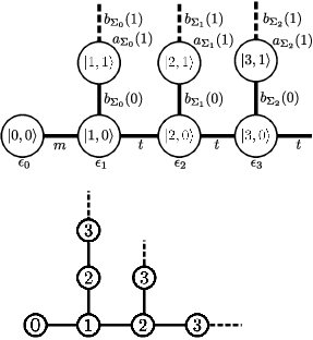
To further illustrate the extension of the Krylov subspace vector , we have added in Fig.4 the tight-binding representation of the Hamiltonian , which has been computed with the in Ref.richler2018inhomogeneous presented I-DMFT method, and which has been used to determine all . Starting Haydock’s recursion from the initial state (electron at site having energy and no phonon modes excited), one then finds
| (12) | |||||
Here states in the energy independent tight-binding representation of are labeled with being the lattice coordinate and being the phonon number (see Fig.4). Projecting on Eq.12 with , respectively one then finds , , and . In the second recursion step one then finds
| (13) | |||||
The set of new recursion coefficients then are , and the new wave function reads
| (14) |
This iterative three-term recurrence procedure is repeated until all recursion coefficients a(n), b(n) and Krylov subspace wave functions are determined.
To conclude, apart from , , which correspond to a electron localized at site , respectively with zero phonon modes excited, all other vectors represents excitations of the many-body system (electron and phonon modes) that progressively spread away from the interface into the acceptor (see Fig.4).
References
- (1) Li G, Zhu R and Yang Y 2012 Nature photonics 6 153
- (2) Günes S, Neugebauer H and Sariciftci N S 2007 Chemical reviews 107 1324–1338
- (3) Lu L, Zheng T, Wu Q, Schneider A M, Zhao D and Yu L 2015 Chemical reviews 115 12666–12731
- (4) Zhu X Y, Yang Q and Muntwiler M 2009 Accounts of chemical research 42 1779–1787
- (5) Drori T, Sheng C X, Ndobe A, Singh S, Holt J and Vardeny Z 2008 Physical review letters 101 037401
- (6) Hallermann M, Haneder S and Da Como E 2008 Applied Physics Letters 93 290
- (7) Shirakawa H, Louis E J, MacDiarmid A G, Chiang C K and Heeger A J 1977 Journal of the Chemical Society, Chemical Communications 578–580
- (8) Morel D, Ghosh A, Feng T, Stogryn E, Purwin P, Shaw R and Fishman C 1978 Applied Physics Letters 32 495–497
- (9) Grancini G, Maiuri M, Fazzi D, Petrozza A, Egelhaaf H, Brida D, Cerullo G and Lanzani G 2013 Nature materials 12 29
- (10) Jailaubekov A E, Willard A P, Tritsch J R, Chan W L, Sai N, Gearba R, Kaake L G, Williams K J, Leung K, Rossky P J et al. 2013 Nature materials 12 66
- (11) Gélinas S, Rao A, Kumar A, Smith S L, Chin A W, Clark J, van der Poll T S, Bazan G C and Friend R H 2013 Science 1239947
- (12) Ballantyne A M, Ferenczi T A, Campoy-Quiles M, Clarke T M, Maurano A, Wong K H, Zhang W, Stingelin-Stutzmann N, Kim J S, Bradley D D et al. 2010 Macromolecules 43 1169–1174
- (13) Hoppe H and Sariciftci N S 2004 Journal of materials research 19 1924–1945
- (14) D’Avino G, Olivier Y, Muccioli L and Beljonne D 2016 Journal of Materials Chemistry C 4 3747–3756
- (15) Tummala N R, Zheng Z, Aziz S G, Coropceanu V and Brédas J L 2015 The journal of physical chemistry letters 6 3657–3662
- (16) Gao F and Inganäs O 2014 Physical Chemistry Chemical Physics 16 20291–20304
- (17) De Sio A and Lienau C 2017 Physical Chemistry Chemical Physics 19 18813–18830
- (18) Falke S M, Rozzi C A, Brida D, Maiuri M, Amato M, Sommer E, De Sio A, Rubio A, Cerullo G, Molinari E et al. 2014 Science 344 1001–1005
- (19) Song Y, Clafton S N, Pensack R D, Kee T W and Scholes G D 2014 Nature communications 5 4933
- (20) Wellein G and Fehske H 1997 Physical Review B 56 4513
- (21) Wellein G and Fehske H 1998 Physical Review B 58 6208
- (22) De Raedt H and Lagendijk A 1983 Physical Review B 27 6097
- (23) Kornilovitch P 1998 Physical review letters 81 5382
- (24) Rozzi C A, Falke S M, Spallanzani N, Rubio A, Molinari E, Brida D, Maiuri M, Cerullo G, Schramm H, Christoffers J et al. 2013 Nature communications 4 1602
- (25) Jeckelmann E and White S R 1998 Physical Review B 57 6376
- (26) Barišić O S 2002 Physical Review B 65 144301
- (27) Potthoff M and Nolting W 1999 Physical Review B 59 2549
- (28) Potthoff M and Nolting W 1999 Physical Review B 60 7834
- (29) Potthoff M and Nolting W 1999 The European Physical Journal B-Condensed Matter and Complex Systems 8 555–568
- (30) Delange P, Ayral T, Simak S I, Ferrero M, Parcollet O, Biermann S and Pourovskii L 2016 Physical Review B 94 100102
- (31) Backes S, Rödel T, Fortuna F, Frantzeskakis E, Le Fèvre P, Bertran F, Kobayashi M, Yukawa R, Mitsuhashi T, Kitamura M et al. 2016 Physical Review B 94 241110
- (32) Jacob D, Haule K and Kotliar G 2010 Physical Review B 82 195115
- (33) Turkowski V, Kabir A, Nayyar N and Rahman T S 2012 The Journal of chemical physics 136 114108
- (34) Bera S, Gheeraert N, Fratini S, Ciuchi S and Florens S 2015 Physical Review B 91 041107
- (35) Athanasopoulos S, Tscheuschner S, Bässler H and Köhler A 2017 The Journal of Physical Chemistry Letters 8 2093–2098
- (36) Aram T N, Asgari A and Mayou D 2016 EPL (Europhysics Letters) 115 18003
- (37) Long R and Prezhdo O V 2014 Nano letters 14 3335–3341
- (38) Ku L C, Trugman S and Bonča J 2002 Physical Review B 65 174306
- (39) Xie Y, Zheng J and Lan Z 2015 The Journal of chemical physics 142 084706
- (40) Pelzer K M and Darling S B 2016 Molecular Systems Design & Engineering 1 10–24
- (41) Gregg B A 2011 The Journal of Physical Chemistry Letters 2 3013–3015
- (42) Anderson P W 1958 Physical review 109 1492
- (43) Haydock R and Mookerjee A 1974 Journal of Physics C: Solid State Physics 7 3001–3012
- (44) Freericks J, Han S, Mikelsons K and Krishnamurthy H 2016 Physical Review A 94 023614
- (45) Haydock R 1980 The recursive solution of the schrodinger equation Solid state physics vol 35 (Elsevier) pp 215–294
- (46) Richler K D, Fratini S, Ciuchi S and Mayou D 2018 Journal of Physics: Condensed Matter 30 465902
- (47) Zheng Z, Tummala N R, Fu Y T, Coropceanu V and Brédas J L 2017 ACS applied materials & interfaces 9 18095–18102
- (48) D’Avino G, Muccioli L, Castet F, Poelking C, Andrienko D, Soos Z G, Cornil J and Beljonne D 2016 Journal of Physics: Condensed Matter 28 433002
- (49) Antropov V, Gunnarsson O and Liechtenstein A 1993 Physical Review B 48 7651
- (50) Faber C, Janssen J L, Côté M, Runge E and Blase X 2011 Physical Review B 84 155104
- (51) Castet F, D’Avino G, Muccioli L, Cornil J and Beljonne D 2014 Physical Chemistry Chemical Physics 16 20279–20290
- (52) Gutknecht M H 2007 A brief introduction to krylov space methods for solving linear systems Frontiers of Computational Science (Springer) pp 53–62
- (53) Ciuchi S, De Pasquale F, Fratini S and Feinberg D 1997 Physical Review B 56 4494
- (54) Hood S N and Kassal I 2016 The journal of physical chemistry letters 7 4495–4500
- (55) Liu A, Zhao S, Rim S B, Wu J, Könemann M, Erk P and Peumans P 2008 Advanced Materials 20 1065–1070
- (56) Poelking C and Andrienko D 2015 Journal of the American Chemical Society 137 6320–6326
- (57) McMahon D P, Cheung D L and Troisi A 2011 The Journal of Physical Chemistry Letters 2 2737–2741
- (58) Poelking C, Tietze M, Elschner C, Olthof S, Hertel D, Baumeier B, Würthner F, Meerholz K, Leo K and Andrienko D 2015 Nature materials 14 434
- (59) Wilke A, Amsalem P, Frisch J, Bröker B, Vollmer A and Koch N 2011 Applied Physics Letters 98 68
- (60) Lanczos C 1950 J. Res. Natl. Bur. Stand. B 45 255–282