Stabilized MorteX method for mesh tying along embedded interfacesJournal: ***
Abstract
We present a unified framework to tie overlapping meshes in solid mechanics applications. This framework is a combination of the X-FEM method and the mortar method, which uses Lagrange multipliers to fulfill the tying constraints. As known, mixed formulations are prone to mesh locking which manifests itself by the emergence of spurious oscillations in the vicinity of the tying interface. To overcome this inherent difficulty, we suggest a new coarse-grained interpolation of Lagrange multipliers. This technique consists in selective assignment of Lagrange multipliers on nodes of the mortar side and in non-local interpolation of the associated traction field. The optimal choice of the coarse-graining spacing is guided solely by the mesh-density contrast between the mesh of the mortar side and the number of blending elements of the host mesh. The method is tested on two patch tests (compression and bending) for different interpolations and element types as well as for different material and mesh contrasts. The optimal mesh convergence and removal of spurious oscillations is also demonstrated on the Eshelby inclusion problem for high contrasts of inclusion/matrix materials. Few additional examples confirm the performance of the elaborated framework.
Keywords:
mesh tying , embedded interface , MorteX method , stabilization , mortar method , X-FEM1 Introduction
The finite element method (FEM) is used to solve a wide range of physical and engineering problems. Based on a variational formulation and a discretized representation of the geometry, this method is extremely flexible in handling complex geometries, non-linear and heterogeneous constitutive equations and multi-physical/multi-field problems. A classification of finite element models can be proposed based on the strategy to represent the boundary of the computational mesh. Classical FE meshes fall into the category of “boundary fitted” (BF) methods, where the boundaries of the physical and computational domains coincide [Fig. 1(a)]. Alternatively, for “embedded/immersed boundary” (EB) methods, the computational domain is a mesh or a Cartesian grid hosting another physical domain [Fig. 1(b)]. Note that material properties or even the governing equations of the host medium and the embedded one can be different. Within the EB method, the geometry contour can be embedded either fully or partially. The BF methods [see Fig. 1(a)] can be used to solve boundary value problems where the boundary conditions are prescribed on surfaces explicitly represented by a mesh. The EB methods [see Fig. 1(b)] can handle a broader class of problems. First, it can be used to solve the same boundary value problems as BF methods but with the boundary represented by a rather general level-set function without explicit discretization of the physical domain. Second, the embedded boundary can serve as a material interface to include features such as inclusions, voids or even cracks for linear/quadratic background meshes [1]. In addition, within the so-called CutFEM [2, 3], debonding of the interface can be taken into account as well as contact between faces. This class of methods can be easily used to create complex geometries [4], however the prescription of boundary conditions on the embedded surface is not straightforward [5, 6]. A particular combination of BF and EB methods shown in Fig. 1(c) deals simultaneously with two or several superposed meshes, which can represent different physics or physical properties. This framework is suited for applications involving fluid-structure interactions (FSI) [7, 8, 9], where the background mesh represents the fluid and the embedded mesh represents the solid.
In this work, we place ourselves in the context of continuum solid mechanics and the finite element method to tie two overlapping meshes: one of these is a boundary-fitted mesh and is referred to as the patch mesh, which is fully or partly embedded in a non-boundary fitted host mesh (the physical domain and the mesh do not coincide). Note that there is no restriction on the number of patches that can be embedded into a host domain. The primary issue addressed here is the continuity of fields across the embedded boundaries. The standard methods to impose stiff continuity or Dirichlet boundary conditions along embedded surfaces include the penalty methods, the method of Lagrange multipliers, Nitsche methods and their variants [10, 11, 12, 13]. Here we consider a framework combining the features of the mortar domain decomposition method and the extended finite element methods (X-FEM) to impose continuity constraints. We refer to this framework as the MorteX method.
The X-FEM is an enrichment method based on the partition of unity (PUM) [14]. In this framework, embedded surfaces, cracks or material interfaces can be modeled without explicit mesh conformity. In X-FEM, it is achieved without compromise on the optimal convergence by means of enrichment functions which are added to the finite element approximation using the framework of PUM. The X-FEM methods are extensively used in applications such as fracture mechanics, voids and inclusions modeling, modeling discontinuities in the porous medium, crack propagation using cohesive elements , simulation of shock wave front and oxidation front propagation, and other applications involving discontinuities both strong and weak [15, 16, 17, 18, 19, 20, 21, 22, 23].
The mortar methods provide us with a comprehensive framework for mesh tying. They are a subclass of domain decomposition methods (DDM) [24, 25, 26, 27], that are tailored for non-conformal spatial interface discretizations [28], and were originally introduced as DDM for spectral elements [29, 30]. The coupling and tying of different physical models, discretization schemes, and/or non-matching discretizations along interfaces can be ensured by mortar methods. The mathematical optimality and applicability of the mortar methods in spectral and finite element frameworks were studied extensively for elliptic problems in [30, 29, 24]. The mortar methods have been successfully adapted to solve contact problems [31, 32, 33, 34, 35].
To ensure displacement continuity across the tied sub-domains, the mortar methods employ Lagrange multiplier fields; as such it is mixed finite element formulation. It is known that the choice of Lagrange multipliers interpolations strongly affects the mesh convergence rate and may lead to loss of accuracy in the interfacial tractions reported for mixed variational formulations as a result of non-satisfaction of Ladyzhenskaya-Babuška-Brezzi (LBB) also called inf-sup condition [36, 37]. Issues resulting from the imposition of Dirichlet boundary conditions using Lagrange multipliers methods has been a topic of interest in various domains, such as the classical FEM [38], Interface-enriched Generalized Finite Element Method (IGFEM) [13], the fictitious domain methods [39], the mesh free methods [40], etc. This problem has also been dealt extensively within the context of the X-FEM. In [10, 41, 42], the authors propose a strategy to construct an optimal Lagrange-multiplier space for the embedded interfaces which permits to apply Dirichlet boundary conditions. As opposed to the strategy of modifying the Lagrange multiplier spaces, the authors in [11] propose a stabilization method to mitigate the oscillatory behaviour of the standard spaces. In the current work, we extend the strategy of modified Lagrange multiplier spaces, which hereinafter will be referred to as coarsening of Lagrange multiplier spaces. This strategy allows us to address specific problems of mesh-locking, which are inherent to mortar methods for overlapping domains, in particular in presence of a strong contrast of material properties in the vicinity of the interface.
Few contributions harnessing the advantages of the mortar method and the X-FEM (but in a different way from what is presented here) are listed below. In [43, 44] the authors used the mortar methods to ensure weak continuity conditions across the interface between a coarser mesh domain and non-intersecting finer mesh surrounding the crack, which in turn is represented by the X-FEM formulation. The tying in this case is limited to the interface with matching geometries but non-conformal discretizations, which is a classical application of the mortar method. A dual mortar contact formulation integrated into X-FEM fluid-structure interaction approach is introduced in [45]. There, the combined X-FEM fluid-structure-contact interaction method (FSCI) allows to compute contact of arbitrarily moving and deforming structures embedded in a fluid.
The proposed method of coupling mortar and X-FEM competes with the volumetric coupling of the Arlequin method [46] and the Polytope FEM for embedded interfaces [47]. The Arlequin method involves superpositioning of the mechanical states in transition zone, and energy redistribution between these states using weight functions. The Polytope FEM involves the decomposition of elements cut by the embedded interface into new polytope elements. This is achieved by the creation of new degrees of freedom (DoFs) along the interface. In [48], the authors used the Nitsche method to impose tying constraints for the overlapping domains circumventing mesh-locking; this method however requires appropriate stabilization.

With the emphasis laid on the interface discretizations handled by the combination of the X-FEM and the mortar methods, many applications could be cited: sub-structuring, inclusion of arbitrary geometrical features into the existing mesh, meshing complex micro-structures, localized mesh refinement near crack tips, general static and dynamic mesh refinement (Fig. 2). However, applications are not limited to mesh tying. In analogy to mortar methods, which were extended to contact problems [31, 49, 50, 51], the method elaborated here can be used to solve contact problems between a virtual surface (represented by the X-FEM) and an explicitly represent surface of the homologue solid [52]. In a separate paper [53] we present the extension of this framework to contact problems, which also allows to treat efficiently wear problems.
The paper is organized as follows. In Section 2 we present the formulation of the interfacial mesh tying problem of overlapping domains; its weak form using the method of Lagrange multipliers is derived in Section 3. Section 4 presents the core methodologies of the X-FEM in terms of inclusion/void modeling and of the mortar discretization for mesh tying problems. The effect of the underlying host mesh interpolations on the tying problem is presented as a case study in Section 5. Two main remedies for mesh locking are presented, namely the triangulation of the blending elements and coarse-graining of Lagrange multipliers, which is detailed in Section 6. In Section 7 we consider two patch tests (tension/compression and bending) to emphasize the inherent problems of embedded boundaries in mixed finite element method. In Section 8 we study the mesh convergence properties of the method using the Eshelby inclusion problem. In Section 9 we illustrate the method’s performance on various applications. In Section 10 we give the concluding remarks and state the prospective works.
2 Mesh tying problem
We consider two open domains and with an overlap region [Fig. 3(a)]. Solid has only outer surfaces which are split into Dirichlet, Neumann and tying boundaries , respectively, such that . We refer to the domain as the “host” domain as it hosts the partially embedded domain . In addition to outer boundaries (the Dirichlet boundary and Neumann boundary ), the host domain contains an embedded boundary (the subscript refers to the “gluing”). We assume that the solids are glued together along the interface formed by the boundaries and ; the physics in the overlap zone is determined by solid . Therefore, in the reference configuration and must remain so in any configuration.
The mesh tying problem is concerned with the enforcement of displacement continuity along the interface and . The standard boundary value problem (BVP) involves ensuring the balance of linear momentum along with the imposed boundary conditions for the two bodies ():
| (1) | ||||
| (2) | ||||
| (3) |
where is the Cauchy stress tensor, represent the density of body forces, is the unit outward normal to and , are the prescribed tractions and displacements. is the effective non-overlapping region of the host domain volume [Fig. 3(b)], where the bar-notation denotes the open domain united with its closure, i.e. . The solution is searched in the appropriate functional space , where is second order Sobolev space. Displacement continuity between the two domains is enforced as:
| (5) |
An equivalent continuum problem is depicted in Fig. 3(b).
3 Weak form
Eqs. (1)-(3) represent the strong form of the standard solid mechanics BVP, and Eq. (5) represents the tying constraints. The weak form of the BVP is accordingly divided into the standard structural part and the contribution from the tying. In the weak form, the requirements on the solution functional space is slightly relaxed compared to the strong form, and an additional field of test functions is selected from another functional space given respectively by :
| (6) | ||||
| (7) |
where denotes the standard first order Sobolev space. In infinitesimal strain formulation, the virtual work corresponding to the structural part is given by:
| (8) |
where is the infinitesimal strain tensor, and are the change in internal energy and the virtual work of forces, respectively. Note that the integration of the virtual internal energy of the host domain is carried out only over the effective volume . The equality constraints (5) are enforced using the method of Lagrange multipliers, whose functions as well as their variations are selected from the space . The multipliers are defined over the surface , which was selected from practical consideration of storing Lagrange multipliers on the explicitly represented surface :
| (9) |
where is the fractional Sobolev space defined over the tying boundary. The Lagrangian of the constrained problem leads to a mixed variational saddle point problem which includes both structural and tying contributions. The variation of the Lagrangian is given by:
| (10) |
where the integration is carried out over the boundary . The first term in square brackets in Eq. 10 represents the virtual work contribution from the tying interface and second term represents the weak form of the equality constraints.
4 Methodology
The evaluation of the internal virtual work restricted to the effective volume of the host solid is accomplished with the X-FEM method. The mortar method is extended to enforce the displacement equality constraint over the interface between the overlapping domains, i.e. between the boundary of the embedded domain (patch) and the corresponding virtual surface of the host solid.
The main features of the proposed method are illustrated on an example shown in Fig. 4. It represents the discretized finite-element setting for the overlapping domains. A discretized11 1 Note that for brevity and simplicity hereinafter we preserve the same notations for discretized entities as were introduced in the continuous problem statement. square patch with a circular hole with surfaces and is embedded into a host mesh . As before the bar notation is used to denote the open domain united with its closure, here . Note that the necessity to consider explicitly the hole as an extra domain comes from the particularities of the problem and was introduced for the sake of avoidance of misinterpretation: the physics inside the contour is fully determined by the patch with a circular hole. The intersection of the patch’s boundary and the host domain represents the virtual surface . The X-FEM is used to account for the virtual work only in the effective domain volume . The mortar method is is brought into play to tie together the two domains and along the interface made of and . Note that in the presented example, the tying boundary is fully embedded.

4.1 Extended finite element method
The virtual surface of the host domain is treated as an internal discontinuity. This is modeled within the X-FEM framework, thereby nullifying the presence of the overlap region in the domain [see Fig. 4(c)]. The X-FEM relies on enhancement of the FEM shape functions used to interpolate the displacement fields. Here the enrichment functions describing the field behavior are incorporated locally into the finite element approximation. This feature allows the resulting displacement to capture discontinuities. The subdivision of the host mesh is defined by indicator function (where is the spatial position vector in the reference configuration in domain ) [54]. The indicator function is non-zero only in the non-overlapping part of domain :
The discontinuity surface can be seen as a level-set defined as follows:
As a result, the indicator function partitions the elements of the host domain into three distinct categories [Fig. 5(a)], namely standard elements, blending elements and discarded elements.
In practice, the enrichment of shape functions in case of void/inclusion problem can be simply replaced by a selective integration scheme [16]. For the standard elements, there is no change in volume of integration and the discarded elements are simply excluded from the volume integration procedure. In order to obtain the effective volume of integration for each blending element, we perform the clipping of the blending elements by the discretized surface [Fig. 5(b)] . The clipping of a single element could result in one or several various polygons22 2 Hereinafter, we assume that all elements use first order interpolation, therefore all edges of elements are straight. It enables us to assume that an intersection or difference of elements can be always represented as one or several polygons. both convex, and non-convex , which represent the effective volumes of integration.

To selectively integrate the internal virtual work in the effective volume only, the resulting polygons are virtually remeshed into standard convex elements (for example, triangles). Note that this remeshing is merely performed to use a Gauss quadrature for integration [Fig. 5(c)], and does not imply the creation of additional degrees of freedom, and as such does not change the topological connectivity of nodes. The displacement field is evaluated using the standard shape functions and the original DoFs; only the integration is changed. To carry out this remeshing, we applied the ear clipping triangulation algorithm [55] to the polygons. The DoFs associated with the elements outside the integration domain [marked with red crosses in Fig. 5(a)] are removed from the global system of equations.
4.2 MorteX discretization
Within the mortar discretization framework, the tied domains are classified into mortar and non-mortar sides. The superscript refers to the mortar side of the interface and to the non-mortar side; the former stores the Lagrange multipliers (dual DoFs) in addition to displacement degrees of freedom (primal DoFs). If the host is selected as a mortar side, the context of the problem becomes similar to the one considered in [10, 41, 42], where it was shown that strong restrictions apply on the choice of Lagrange multiplier spaces in order to fulfill the inf-sup condition. The algorithm for construction of such spaces is not straightforward. Therefore, to avoid these difficulties, we select the patch side as the mortar surface, which provides us with a more flexible setting. This choice was already reflected in the fact that the host boundary was chosen as the integration side for tying conditions (10). However, under specific problem settings, the choice of employing standard interpolation functions for the Lagrange multipliers on the embedded interface still leads to spurious oscillations of interfacial tractions. Remedies for this problem will be discussed in Section 7.
Displacements on the mortar side are given by classical one-dimensional shape functions with the interpolation order equal to that of the underlying mesh:
| (11) |
where is the number of nodes per mortar element’s edge and is the parametric coordinate of the mortar side. The displacements along the virtual surface running through the host mesh elements are characterized by the two dimensional host mesh interpolations, and can be expressed as follows:
| (12) |
where is the one-dimensional parametric coordinate of integration segment of non-mortar side, are the classical two-dimensional parametric coordinates of the host element, and is the number of nodes of this element. The use of two-dimensional interpolation on the non-mortar side marks the difference between the classical mortar and the presented MorteX frameworks. The Lagrange multipliers (defined on the mortar side) are interpolated using shape functions :
| (13) |
where can be less than or equal to . It enables to select shape functions for dual variables independently of the primal shape functions.
Few remarks could be made here. We need first to introduce the notion of segment: it is a straight line whose vertices can either be a clip intersection33 3 The clip intersection points are located on the edges of blending elements intersected by the virtual surface . or a kink point, the later being a node of the mortar side lying inside the host element. Note that segments are defined both on mortar and non-mortar sides as they coincide. Since a host element can be intersected by several patch segments [Fig. 6 (a)], the functions , can be piece-wise smooth, which implies that the underlying displacement (and coordinate) can also be piece-wise smooth. Second remark: if the host elements are quadrilateral, then each segment interpolation is given by , where is the mortar interpolation order, and is the non-mortar interpolation order; the later is augmented by one since the virtual interface passes inside the element, where the interpolation order in quadrilateral 2D elements is one order higher than along the edges. For a triangular host mesh, the interpolation order is simply the product of interpolation orders of the host and patch meshes . To give an example, let us assume that the patch mesh is linear and the host mesh is linear quadrilateral; then let us imagine that a host element is cut into two parts by a (straight) patch segment. Then the displacement in the host element along this straight segment will be second order polynomial function of the parameter [see Fig. 6(b)]. However, the displacement along such a cut would remain linear for triangular linear host elements [see Fig. 6(c)].
4.2.1 Mortar interface element
A mortar element is formed with a single mortar segment (on the patch side) and a single non-mortar element (on the host side). Each tying element consists of nodes, from the mortar segment, and from non-mortar element, and stores Lagrange multipliers, where is the spatial dimension. The choice of is guided by the inf-sup condition requirement of the discrete Lagrange multiplier spaces (usually ).
Substituting the interpolations (11), (12), (13) into the weak form (10) and extracting only the terms related to the mesh tying of a single mortar element, we obtain
| (14) |
| (15) |
where and are the mortar integrals evaluated over the
mortar-side segments , where is the current host
element forming the mortar element.
(16)
(17)
The nodal blocks of the mortar matrices denoted as ()
and () can be expressed as:
| (18) |
| (19) |
where, is the identity tensor of the spatial dimension of the problem. Using matrix notations, Eq. (15) reads
| (20) |
where arrays store current values of associated nodal primal (on mortar and non-mortar sides) and dual (mortar) DoFs:
whereas their variations are denoted . The tangent operator for the mortar interface element is obtained by taking the derivatives of (20) with respect to its DoFs:
| (21) |
This tangent operator has zero blocks for primal DoFs, non-zero blocks to link primal with dual DoFs, and zero blocks on the main diagonal, which is the typical structure of a saddle-point system.
4.2.2 Evaluation of mortar integrals
The evaluation of mortar integrals is performed over segments (see Figs. 6,7). The evaluation of the integrals (16) is straightforward, as it involves the product of shape functions from the mortar side only. In contrast, the integral (17) combines shape functions from both mortar and non-mortar sides. The evaluation of this integral requires a mapping between the mortar and non-mortar sides.
The integration domain is parametrized by (Fig. 7), which needs to be linked with the parametrization of the mortar side, which is given by:
| (22) |
where and define the limits of the integration on the mortar side as shown in Fig. 7. To evaluate the integrals using the Gauss quadrature, we need to find the location of Gauss points in terms of mortar () and non-mortar () parametrization. While the former is straightforward using (22), the latter can be done by solving the following equation:
| (23) |
where the physical location of the Gauss point is given by . With these notations, the mortar integrals can now be evaluated using the Gauss quadrature rule as:
| (24) |
| (25) |
where as previously , , and is the number of Gauss integration points, are the Gauss weights, is the Jacobian of the mapping from the parent space to the real space including the adjustment of the integral limits:
| (26) |
5 Intra-element interpolation of displacements in the host mesh
For the overlapping domains the coupling is made between the patch mesh boundary and virtual surface running through the host mesh elements. This is reflected in the mortar matrix (25) that contains the integral of a product of volumetric (in the host mesh) and surface (patch mesh) shape functions. To demonstrate the effect of the interpolation choice, we use the set-up shown in Fig. 8 (a). The following dimensions are used: mm, mm, mm and mm. A uniform pressure of MPa is applied on the top surface of . The meshes and are tied along the interface .

The domain is discretized with a triangular (T1) and two quadrilateral (Q1, Q2) elements, all elements use first order interpolation, and the patch domain is discretized into a rectangular elements [Fig. 8(b)]. The two domains are made of the same linearly elastic material ( GPa, ); the reference solution for the selected boundary conditions is a uniform stress field ( and ) whether it be under plane strain or plane stress formulation. Of course, the displacement along the tying line is uniform. However, as shown in Fig. 9 the selected discretization does not allow to obtain the reference solution. The solid line in Fig. 9 shows the resulting vertical displacement along the tying line ; it consists of a combination of linear and non-linear portions. We hypothesize that the inability to reproduce the reference solution is somehow related to the interpolation order of displacement in host elements. As seen from the figure, the order of the solution is matching the maximum available interpolation order of displacements . This maximum interpolation order is one () along any straight line inside a linear triangle (T1). However, this order raises to two () along straight lines inside quadrilateral elements, as long as both parent coordinates and change along these lines (Q2). This is not the case in Q1 (), where one of parent coordinates remains constant along the virtual interface, i.e. or .
This observation motivates us to test triangulation of blending element to limit the maximum interpolation order in host element to one (). This operation does not change the number of DoFs and is easy to handle in practice. This procedure enables us to obtain the reference solution in the considered case as demonstrated in Fig. 9. The general applicability of this method will be tested in the following sections.
6 Coarse Grained Interpolation (CGI) of Lagrange multipliers
The stability of the proposed mixed formulation is guided by the requirement to satisfy the inf-sup condition [36], which is not a trivial task. For example, the use of Lagrange multipliers with standard interpolation leads to non-physical oscillations along the interface when used to enforce Dirichlet boundary conditions [38]. Having a much stiffer patch than the host material represents a case approximately similar to the imposition of Dirichlet boundary conditions, therefore in most presented examples stiffer patch will be used. The technique presented in [10, 41] for the X-FEM framework, involves coarsening of the Lagrange multipliers to avoid spurious oscillations. This is achieved by algorithmically selecting nodes referred to as "winner nodes" along the Dirichlet boundary. The algorithm favors nodes close to the boundary, or nodes from which many edges intersecting the boundary emanate. The Lagrange multiplier space is built using the winner nodes. The size of the multiplier space is the size of the winner nodes set. Inspired from this technique, we suggest to coarse grain the interpolation of Lagrange multipliers (dual DoFs) to avoid spurious oscillations. In Fig. 10, for example, the number of mortar nodes (each of which carries Lagrange multipliers in the standard approach) per host element considerably outnumbers the associated DoFs to render the associated constraints independent of physical deformations the host elements allow [48]. Therefore the system shown in this figure is overconstrained and requires an appropriate stabilization. Coarse graining of Lagrange multiplier interpolation functions enables to reduce the number of constraints and thus improves the problem stability. In this approach, not every mortar node is equipped with a Lagrange multiplier. Therefore, the interpolation functions become non-local, i.e. they span more than one patch segment. For this purpose, we choose a 1D parametric space , spanning multiple mortar-side segments. Such parametrization can be chosen such that length of the corresponding super-segment in the physical space is comparable to the size of host elements. As shown in Fig. 10(a), the mortar-surface is segmented into three super-segments of lengths and . The end nodes of these segments are termed the “master” nodes (they carry the dual DoFs ), other mortar-nodes are termed “slave” nodes. We introduce the local coarse-graining parameter that determines the number of segments contained in a super-segment, and thus determines the number of slave nodes per super-segment. In Fig. 10(a), the coarse-graining parameter takes the values , for the super-segments of lengths and , respectively.
In theory, the coarse graining is achieved through defining dual DoFs only on master nodes. In practice, this can also be done by keeping the Lagrange multipliers at all mortar nodes and using a multi-point constraint (MPC) to enforce a linear interpolation between the master nodes. Hence, for a given slave node, the dual DoFs are given by:
| (27) |
The parametrization of the super-segment can be chosen such that : , where the numerator represents the spacing between two mortar (patch) nodes in the coarse-grained parametric space and corresponds to the physical length of the corresponding segment. An average ratio of number of mortar segments per number of blending elements, which is termed “mesh contrast” , can be used to guide the selection of the coarse-graining parameter : for example, (18 mortar segments per 3 host elements) in the example shown in Fig. 10. The coarse-graining parameter , for an open mortar surface, can take values in the range , where is the number mortar segments; for a closed mortar surface the upper limit is one less.
The optimal choice of coarse-graining parameter is studied on particular problem settings in Sections 7 and 8 for open and closed mortar surfaces. The limit case corresponds to the standard Lagrange interpolation (SLI). For the case of approximately regular discretization on both sides, a global coarse-graining parameter can be chosen, and its value is set to be approximately equal to the mesh contrast parameter as shown in Fig. 10(b). In case of non-regular mesh discretizations on mortar or/and on host sides, the coarse-graining parameter should be selected element-by-element according to the local mesh contrast as shown in Fig. 10(a). However, in all the examples considered below, we use regular discretizations, and thus the global coarse-graining parameter will be used.
7 Patch tests
In this section, the algorithms introduced in the previous sections, implemented in the finite element suite Z-set [56], are tested on simple problems of tied overlapped domains of different discretizations and different material contrasts subject to bending or tensile/compressive boundary conditions: the patch mesh is and the host mesh is . Linear elastic material properties are used for both the patch () and the host (). The geometric set-up of the patch and host domains are illustrated in [Fig. 11 (a)]. The following two extreme cases will be considered: Case 1. a finer and stiffer patch mesh is superposed onto the host mesh, and Case 2. a coarser and stiffer patch mesh is superposed onto the host mesh.
These two particular cases are chosen for the validation since they are prone to severe manifestations of the mesh locking [48] as in the case of enforcing Dirichlet boundary conditions using Lagrange multipliers along embedded surfaces [10, 41, 42]. Additionally, the host domain is meshed with ”distorted“ quadrilaterals which is classical in patch test studies to exacerbate potential anomalies. Moreover, as was shown by a simple example Section 5 the tying along distorted quadrilateral elements is prone to considerable errors if the mortar-type tying is used directly. The material contrast is introduced by choosing , and GPa, both domains have the same Poisson’s ratio . The discretizations for the two cases are shown in Fig. 11 (b, c). The mesh contrast and and the number of mortar segments and are used for Case 1 and 2, respectively. Note that all the stress fields along the tying interface, which are presented on the plots below, are found by the data extrapolated from Gauss points and averaged at mortar nodes.

7.1 Tension/compression patch test
A uniform pressure is applied on the top surface, the bottom surface is fixed in all directions [Fig. 12(a)]. This is a classical patch test in contact mechanics, which is used here to test the tying of different materials. This material contrast requires additional lateral conditions (lateral sides are fixed in normal direction ) to avoid singularities at extremities of the interface. The reference solution for is a uniform field . As expected, in case of stiffer and finer patch mesh (Case 1), spurious oscillations are observed. They have large amplitude that reaches % of the reference solution, moreover, they are not confined to the interface but propagate into the bulk [Figs. 13(a), 14(a)]. In case of stiffer and coarser patch mesh (Case 2), the spurious oscillations are of considerably lower amplitude (under %), they are rather localized in the host mesh in close vicinity of the interface and do not extend in the patch mesh [Figs. 13(b), 14(b)].

In order to quantify the improvement achieved with the suggested coarse grained interpolation (CGI) and with triangulation technique, we introduce the -norm of the error in the stress component:
| (28) |
where the norm means , where are the -coordinate of mortar nodes in the reference configuration, and is the length of the surface . In Fig. 15 we demonstrate the performance of the CGI technique. As seen from the figure, the error in stress greatly reduces compared to the standard interpolation (SLI), when coarse-graining parameter increases. However, the error saturates at and the convergence to the reference solution is missing. On the contrary, the triangulation technique (Fig. 16) enables to achieve a superior precision as shown in Figs. 15(a) and 17.

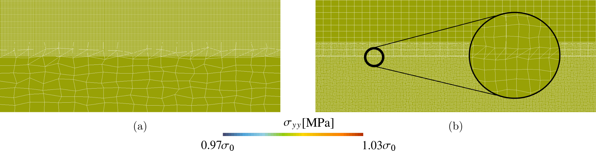
7.2 Bending patch test
A linear distribution of pressure
| (29) |
with MPa is applied on the bottom surface, while keeping the top surface fixed in vertical direction, only the corner point is fixed in horizontal direction, the lateral sides remain free [Fig. 12 (b)]. The same linear distribution of the vertical stress component (29) through the two solids should take place. This case study (Case 1, 2) was inspired from the work [48], where the authors also used the combination of the mortar method and the selective integration. It was shown that Case 1, in particular, results in high-amplitude spurious oscillations in the interface contrary to Case 2 that has a smoother stress profile along the interface. Under the standard Lagrangian interpolation set-up we could reproduce similar results, see Fig. 18, 19. These oscillations could be removed with Nitsche method provided some adjustment of the stabilization penalty parameters on each side of the interface [48]. We demonstrate below that using the coarse-grained interpolation for Lagrange multipliers, as suggested in Section 6, also permits avoiding these oscillations in the MorteX framework. As discussed in Section 6, the choice of the optimal coarse-graining parameter is governed by local or global mesh contrast, which can be easily determined either for every segment or for the whole interface. It renders the choice of the coarse-graining parameter fully automatic. Contrary to the stabilized Nitsche method, no knowledge about local material contrast is needed.

In Fig. 20, the vertical stress component is shown for the Case 1 when the coarse-graining parameter for Lagrange multipliers is set to (a) and (b) . It is clearly seen in the figures that does not sufficiently relaxes the over-constraining of the Lagrange multipliers space (we recall that ) to obtain a smooth reference solution, even though the amplitude of oscillations is slightly reduced compared to standard Lagrange multipliers, which can be seen in Fig. 21(a) where the standard solution (obtained with the standard interpolation of Lagrange multipliers SLI) is compared with the coarse-grained interpolation (CGI). With the coarse-graining parameter we obtain a much improved result comparable to the reference solution.
The relative error Eq. (28) is shown in Fig. 21(b) for different values of . The error becomes acceptable only for , however, the accuracy of the solution constantly improves with a further increase of . The fast drop of the error for is associated with the graduate removal of spurious oscillations in the stress distribution, whereas for improves further the error by better approximation of stresses at extremities of the interface. Since the reference stress distribution is linear, only two Lagrange multipliers are sufficient to capture it, leading to an error reduction up to . In general, as will be shown later, too coarse a representation of Lagrange multipliers leads to deterioration of the solution (see Section 8). The triangulation of blending element is also tested in the bending patch test, see Figs. 22. In contrast to the compression patch test, triangulation here does not help with the removal of spurious oscillations.


7.3 Summary of patch tests
Here, we present the ensemble of patch-test results for various combinations of host/patch meshes and material contrasts. As before, we consider two cases: Case 1 corresponds to a fine patch mesh [mesh-density contrast , Fig. 23(a)] which is tied with a coarser host mesh made of triangular, aligned or distorted quadrilateral elements Fig. 23(b,c,d), respectively. Results of Case 1 are presented in Table 1. In Case 2, the patch mesh [mesh-density contrast , Fig. 24(a)] is coarser than the host mesh, which again can be made of triangles, aligned or distorted quadrilateral elements, see Fig. 24(b,c,d), respectively. Results of Case 2 are presented in Table 2. Softer () and stiffer () patch materials are compared to the host material were considered. We also tested different interpolation order (p0 and p1) for standard Lagrange interpolation (SLI), and p1-interpolation for coarse-grained interpolation (CGI) in which the coarse-graining parameter takes its maximum value . The table clearly demonstrates that the tying performance is strongly dependent on the type of patch test. Cases which show a small error in bending test can demonstrate a slightly higher error in compression test as in case , for distorted quads with CGI scheme. However, with a high fidelity it could be stated that if the tying method passes the bending patch test then it passes the compression patch test. The inverse is, in general, false. Interestingly, the triangulation of quadrilateral elements can considerably increase the error in case of SLI scheme, it does not happens with the CGI scheme. Clearly, from these tables it can be concluded that the CGI scheme outperforms the standard SLI scheme (both p0 and p1) in all studied combinations of mesh, element types and patch-test type (48 tests in total).

| Triangulation | Dual | ||||
|---|---|---|---|---|---|
| Host-mesh type | of blending | interpolation | error | error | |
| elements | (bending patch test) | (compression patch test) | |||
| 1000 | Triangles | No | SLI (p0) | 1.668e+01 | 3.57e-06 |
| Aligned quads | No | 3.357e-01 | 0.00 | ||
| Distorted quads | No | 2.95e+00 | 1.064e+00 | ||
| Yes | 7.66e+00 | 4.76e-05 | |||
| 1000 | Triangles | No | SLI (p1) | 1.266e+01 | 3.55e-06 |
| Aligned quads | No | 2.789e-01 | 0.00 | ||
| Distorted quads | No | 2.30e+00 | 7.627e-01 | ||
| Yes | 4.786e+00 | 4e-06 | |||
| 1000 | Triangles | No | CGI (p1) | 4.53e-05 | 0.00 |
| Aligned quads | No | 4.51e-05 | 0.00 | ||
| Distorted quads | No | 2.4e-04 | 1.e-3 | ||
| Yes | 2.3e-04 | 3.e-4 | |||
| 1.e-3 | Triangles | No | SLI (p0) | 2.192e-01 | 0.00 |
| Aligned quads | No | 2.192e-01 | 0.00 | ||
| Distorted quads | No | 2.186e-01 | 2.9e-05 | ||
| Yes | 2.192e-01 | 2.4e-05 | |||
| 1.e-3 | Triangles | No | SLI (p1) | 2.193e-01 | 0.00 |
| Aligned quads | No | 2.194e-01 | 0.00 | ||
| Distorted quads | No | 2.191e-01 | 1.15e-05 | ||
| Yes | 2.194e-01 | 0.00 | |||
| 1.e-3 | Triangles | No | CGI (p1) | 4.51e-05 | 0.00 |
| Aligned quads | No | 4.51e-05 | 0.00 | ||
| Distorted quads | No | 2.4e-04 | 2.8e-4 | ||
| Yes | 2.3e-04 | 2.8e-4 |

| Triangulation | Dual | ||||
|---|---|---|---|---|---|
| Host-mesh type | of blending | interpolation | error | error | |
| elements | (bending patch test) | (compression patch test) | |||
| 1000 | Triangles | No | SLI (p0) | 2.122e-01 | 2.34e-05 |
| Aligned quads | No | 2.113e-01 | 0.00 | ||
| Distorted quads | No | 2.114e-01 | 3.58e-04 | ||
| Yes | 7.66e+00 | 4.76e-05 | |||
| 1000 | Triangles | No | SLI (p1) | 2.493e-01 | 1.63e-05 |
| Aligned quads | No | 2.481e-01 | 0.00 | ||
| Distorted quads | No | 2.483e-01 | 5.00e-04 | ||
| Yes | 4.786e+00 | 4e-06 | |||
| 1000 | Triangles | No | CGI (p1) | 6.00e-04 | 7.42e-07 |
| Aligned quads | No | 6.00e-04 | 0.00 | ||
| Distorted quads | No | 6.00e-04 | 1.75e-06 | ||
| Yes | 6.00e-04 | 0.00 | |||
| 1.e-3 | Triangles | No | SLI (p0) | 1.702e-01 | 0.00 |
| Aligned quads | No | 1.702e-01 | 0.00 | ||
| Distorted quads | No | 1.702e-01 | 1.72e-06 | ||
| Yes | 2.192e-01 | 2.4e-05 | |||
| 1.e-3 | Triangles | No | SLI (p1) | 1.734e-01 | 0.00 |
| Aligned quads | No | 1.734e-01 | 0.00 | ||
| Distorted quads | No | 1.735e-01 | 0.00 | ||
| Yes | 2.194e-01 | 0.00 | |||
| 1.e-3 | Triangles | No | CGI (p1) | 5.5e-04 | 0.00 |
| Aligned quads | No | 5.5e-04 | 0.00 | ||
| Distorted quads | No | 5.5e-04 | 0.00 | ||
| Yes | 5.5e-04 | 0.00 |
8 Circular inclusion in infinite plane: convergence study
Having demonstrated a general good performance of the coarse-graining interpolation, here we carry out a mesh-convergence study. We focus on the worse case scenario (see Section 7) when the patch mesh is finer and stiffer than the host mesh. We consider a circular inclusion embedded in an infinite softer matrix in plane strain formulation, and subject to a uniform traction applied at infinity [57, 58, 59]. This particular problem represents a sub-case of a general Eshelby problem of an ellipsoidal inclusion in a matrix [60, 61]. Fig. 25(a) shows the used computational set-up: a circular inclusion (patch) with radius mm, centered at origin, is superposed on a matrix (host) represented by a square of side mm (). Linear elastic material properties are applied to both the inclusion () and the matrix (). The inclusion is made more rigid than the matrix by choosing , GPa, the same Poisson’s ratio is used for both . A uniform pressure MPa is applied on the right side as shown in Fig. 25(a), displacements on the left side are fixed in horizontal direction and the lower left corner is fixed. The inclusion patch is tied to the host matrix along the boundary of the inclusion .
The analytical solution for the stress state inside and outside the inclusion is given below in polar coordinates () [58]. Stress components inside the inclusion () are given by:
| (30) | ||||
| (31) | ||||
| (32) |
where,
| (33) |
Outside the inclusion (), the stress components are given by:
| (34) | ||||
| (35) | ||||
| (36) |
where
| (38) |
For the considered plane strain formulation the material constants and are given by
| (39) |
8.1 Mesh convergence
We are particularly interested in the stress state along the tying boundary () where possible spurious oscillations take place. The distribution of the radial stress component at can be obtained either from44 4 Note however that is not continuous across the interface Eqs. (30) or (34). This analytical solution is compared with the numerical one obtained using MorteX method along the interface , for which [see Fig. 25(b)]. For this purpose we use the error norm as in (28) defined along :
| (40) |
where is the analytical solution, and is the radial component of Lagrange multiplier vector obtained by projecting it on the radial basis vector of polar coordinates . The mesh refinement is carried out maintaining a constant mesh contrast between the patch and the host meshes, i.e. the ratio of the mortar segments to the number of blending elements is fixed to be (Fig. 26); the number of mortar segments was varied (in Fig. 25(b) and 26 the coarsest mesh with is shown). Four cases are considered for this convergence study: (i) standard p1 interpolation (SLI) is used for Lagrange multipliers; (ii) blending elements are triangulated; (iii) coarse grained interpolation (CGI) is used for Lagrange multipliers with various coarse graining parameter ; (iv) both triangulation and coarse graining are used.

We recall that to represent the interfacial tractions in compression and bending patch tests one or two Lagrange multipliers, respectively, were enough. In contrast to these patch tests, here the stress distribution is no longer affine along the tying interface, therefore it is expected to obtain a more practical result for the selection of the coarse graining parameter , which ensures optimal convergence. Results obtained for mesh contrast and for and different coarse-graining are shown in Fig. 27. The oscillations are clearly seen near the inclusion/matrix interface, especially inside the inclusion. However, for high enough these oscillations are completely removed and a uniform stress field is recovered inside the inclusion. A quantitative convergence study is presented in Fig. 28(a). It clearly demonstrates that for standard interpolation (SLI, i.e. ) or coarse-grained interpolation (CGI) used with small values of , the presence of spurious oscillations induces very high errors in interfacial tractions [see Fig. 29(a)]. When , the error reaches its minimum. This is due to the fact that for the given discretization, this level of coarse graining offers an appropriate balance between on the one hand the relaxation of the over-constraining of the Lagrange multipliers, and on the other hand the ability to accurately describe the complex traction field at the interface. For higher values of the error increases again because of too coarse representation of interfacial tractions. It is thus expected that, in general case, there exists a range for which ensures oscillation free and accurate enough solution. It is also expected that optimal is determined by the global mesh density contrast . However, as demonstrated in Fig. 26, the local mesh density contrast can be more pronounced than the average one, therefore it is expected that the optimal value of coarse graining parameter lies in the range ; for the considered case the error is minimized for , probably, the optimal value lies in between. The effect of optimal is clearly demonstrated in Fig. 29(b) where interfacial tractions for different are plotted.

For the fixed mesh contrast and optimal and sub-optimal , the mesh convergence was carried out with meshes of different densities . In Fig. 28(b) we plot the error decay with decreasing mesh size, for which we select the length of mortar edge normalized by the total length of the interface . For the selected error-measure along the inclusion/matrix interface, the standard interpolation for Lagrange multiplier (SLI) results in optimal convergence (). However, even though the convergence is optimal, the error remains very high due to the spurious oscillations, implying that an excessively fine mesh would be required to achieve an acceptable error. For example, to reach % in case of SLI, 51 200 elements on the mortar side would be needed. Moreover, for quadrilateral host mesh in absence of triangulation of blending elements, the convergence is lost for very fine meshes. In contrast, the coarse graining technique (CGI) used with optimal results in the error below %, even with the coarsest mesh used in our study . At the same time, the optimal convergence is preserved. As expected, the triangulation of the blending elements slightly deteriorates the quality of the solution, but preserves the optimality of the convergence.
The effect of the parameter on the amplitude of spurious oscillations is demonstrated in Fig. 30. For a fixed host-mesh discretization we increase the number of mortar edges , which correspond to . Fig. 30(a) demonstrates the increase in the amplitude of oscillations with increasing mesh contrast for SLI interpolation. The removal of spurious oscillations with the CGI scheme is shown in Fig. 30(b) for reasonable choice of coarse graining parameter for , respectively.
9 Numerical examples
In this section we illustrate the method of mesh tying along embedded interfaces in light of potential applications. In all the presented examples, we use a linear elastic material model under plane strain assumption. All the problems are solved in the in-house finite element suite Z-set [56]. All triangular and quadrilateral elements used in simulations possess three and four Gauss points for integration, respectively. The triangulated blending elements also use three Gauss points. The MorteX interface uses three integration points to evaluate the MorteX integrals.
9.1 Plate with a hole
As a first example, we solve the problem of a square plate with an embedded square patch containing a circular hole, which was used to illustrate the method in Section 4 (Fig. 4). This example demonstrates the ease with which arbitrary geometrical features can be included into the host mesh. Classically, in the X-FEM method a void can be easily included in the host mesh, however, in the vicinity of the void a stronger stress gradients take place, therefore the mesh around the void should be properly refined. It can be easily achieved by surrounding the void with a finer patch mesh, as done here, and by embedding this refined geometry in a coarse host mesh. The geometric dimensions used in the problem are the following: the plate’s side is mm, the hole’s radius is mm and the patch’s side is mm [Fig. 31(a)]. The patch and the host are made of the same material with Young’s modulus MPa and Poisson’s ratio . The left edge of the host domain is fixed in (), the lower left corner is fixed, and a uniform traction MPa is applied on the right edge, the upper and lower boundaries remain free . For comparison purposes, a reference solution is obtained with a classical monolithic mesh [Fig. 31(c)].


Fig. 32(a) shows a rather smooth contour of stress component , which was obtained using MorteX tying with SLI scheme. However, the seemingly smooth stress field near the interface, exhibits oscillations near the interface as can be seen in Fig. 32(b), where was plotted over a part of the interface . These oscillations have a smaller amplitude than in cases with high material contrast, and as previously, they can be efficiently removed when coarse-grained interpolation CGI is used, what is shown in the same figure. Coarse-graining parameter appears to be sufficient to remove them. Note that the slight difference between the MorteX tying and the monolithic mesh comes from inherently different extrapolation/interpolation of stresses to the interface nodes.
9.2 Crack inclusion in a complex mesh
In many engineering applications, the solids are subjected to cyclic loads and therefore modeling of structures with fatigue cracks appears essential for computational lifespan prediction. The structural finite element analysis can indicate potential locations of the onset of fatigue cracks, however, insertion of cracks is not always trivial [62, 63], especially, in the common case where the original CAD model is not available . Moreover, the position of the onset of the crack is subjected to statistical perturbations, therefore it is often of interest to probe various scenarios in which the crack starts at different locations. Within the proposed framework, studying various fracture scenarios (crack in this case) merely implies placing the patch at a different location on a host mesh, avoiding potential creation of conformal geometries. Here we demonstrate an example of incorporating a crack in a model blade-disk fir-tree connection subject to a vertical tensile load. The frictionless contact is handled using the augmented Lagrangian method in the framework of the standard mortar method. The following dimensions [see Fig. 33(a)] are used for the blade disk assembly: mm, mm, mm and mm. The Young’s modulus is MPa and for the blade, disk, and the patch containing the crack of length mm. A vertical displacement mm is applied on the top surface of the blade. In Fig. 33(a) we present the resulting stress field for the case of intact structure and for the case of a structure with embedded crack, respectively. As seen in the later case, the stress fields are very smooth across the tying interface (shown as white dashed boundary) ensured by MorteX with SLI only. The coarse graining is not needed here as the mesh densities are comparable and the same material is used for the patch and for the host. Similarly to the presented case of crack insertion, the method can be used in general for introducing various other geometric features into the existing mesh. Using the MorteX method, the location/orientation of these features can be adjusted with ease and without remeshing to perform a sensitivity analysis.

9.3 Multi-level submodeling: patch in a patch
In this example we demonstrate the ability of the MorteX method to handle multi-level overlapping domains, i.e. when an embedded patch mesh hosts other domains. In Fig. 34(a) we present such a scenario where a patch with a notch () is embedded into a host domain , both made of the same material. At the same time, the patch itself hosts 2 circular inclusions (), which are stiffer than the surrounding material. The following dimensions are used: mm, mm, mm, mm, mm, and mm. The material properties used are: MPa, MPa, MPa, MPa (the upper indices correspond to the domains respectively). A Poisson’s ratio of is used for all the domains. A vertical displacement mm is applied on top surface of the , while the left surface is fixed in the direction and bottom is fixed in all directions. The contour plots of for the cases of SLI and CGI are shown in Fig. 35(a) and (b), respectively. The oscillations in the stress are distinctly seen in case of SLI, but they are removed by applying CGI with . Fig. 36 compares along , , which form portions of matrix/inclusion interfaces. This example illustrates the case where a host mesh with embedded domains of different material properties can be dealt within CGI MorteX scheme. Note that in contrast to the Nitsche method where the stabilization parameter needed to avoid mesh locking is dependent on the local material contrasts [48], the CGI stabilization does not require the knowledge of this contrast. In the CGI scheme, knowing a local or a global contrast of mesh densities across the tying interface is enough to automatically select the coarse graining parameter , which efficiently stabilizes the mixed formulation and removes spurious oscillations present in the standard mortar scheme.


10 Conclusion
We presented a unified framework for mesh tying between overlapping domains. This framework was entitled MorteX as it combines features of the mortar and X-FEM methods. As known, the resulting mixed finite element problem may be prone to mesh locking phenomena especially for high material or mesh-density contrasts between the host and the patch meshes. Manifestation of the emerging spurious oscillations for different element types and various material as well as mesh contrasts was illustrated on two patch tests (bending and compression) and on selected examples. These oscillations strongly deteriorate solution in the vicinity of interfaces resulting in poor mesh convergence. Even though triangular elements help to avoid oscillations in compression patch tests, they do not perform well in bending patch test, nor in more complicated examples. These oscillations comes from the over-constraining of the interface in case of mesh-density contrast, when few mortar-side nodes located on the patch mesh are tied to displacement field of a single host element. To get rid of the resulting mesh locking, we suggested to coarse-grain interpolation (CGI) of Lagrange multipliers by interpolating the associated field along few mortar edges. It implies that only every node along the mortar side stores a Lagrange multipliers and a linear interpolation is used in between. The value of coarse-graining spacing parameter controls the performance of the scheme. If is too small compared to mesh-density contrast, the spurious oscillations persist as in standard interpolation of Lagrange multipliers (SLI). If the value of is too high, the spatial variation of resulting interface tractions cannot be captured properly. Therefore, in general problem, there exists an optimal choice for the spacing parameter which can be automatically determined either by local mesh-density contrast between the patch and the host mesh or by the global mesh-density contrast. The performance of the MorteX method with coarse-grained interpolation was demonstrated on Eshelby problem for a stiff inclusion in a softer matrix (elastic contrast of 1000). Few other examples, demonstrating the ease with which the method can be used for: submodeling, local mesh refinement and inclusion of arbitrary geometrical features in the existing mesh, without remeshing. Among these examples, a multi-level/hierarchical overlapping is shown, where a patch is inserted into a host mesh, which in turn is inserted into another host mesh. The MorteX method equipped with CGI demonstrates a very good performance, removes the mesh locking oscillations, and ensures optimal convergence. The important feature of the method is that its stabilization requires knowledge of local mesh densities only, thus it presents a good alternative to the Nitsche method, which requires stabilization constructed on a priori knowledge of material stiffness in the interface. In analogy with the classical mortar method, the MorteX method can be extended to handle contact problems along virtual interfaces embedded in a mesh; this extension is presented in a separate paper [53].
Acknowledgment
The authors acknowledge financial support of the ANRT (grant CIFRE no 2015/0799). We are also grateful to Nikolay Osipov and Stéphane Quilici from the Z-set team for their help with the implementation of the method.
References
- [1] T. P. Fries, Higher-order conformal decomposition FEM (CDFEM), Computer Methods in Applied Mechanics and Engineering 328 (2018) 75 – 98.
- [2] E. Burman, S. Claus, P. Hansbo, M. G. Larson, A. Massing, CutFEM: Discretizing geometry and partial differential equations, International Journal for Numerical Methods in Engineering 104 (7) (2015) 472–501.
- [3] S. Claus, P. Kerfriden, A stable and optimally convergent LaTIn-CutFEM algorithm for multiple unilateral contact problems, International Journal for Numerical Methods in Engineering 113 (6) (2018) 938–966.
- [4] T. Belytschko, C. Parimi, N. Moës, N. Sukumar, S. Usui, Structured extended finite element methods for solids defined by implicit surfaces, International journal for numerical methods in engineering 56 (4) (2003) 609–635.
- [5] F. Duboeuf, E. Béchet, Embedded solids of any dimension in the X-FEM. Part I – Building a dedicated P1 function space, Finite Elements in Analysis and Design 130 (2017) 80 – 101.
- [6] F. Duboeuf, E. Béchet, Embedded solids of any dimension in the X-FEM. Part II –Imposing Dirichlet boundary conditions, Finite Elements in Analysis and Design 128 (2017) 32 – 50.
- [7] F. P. T. Baaijens, A fictitious domain/mortar element method for fluid–structure interaction, International Journal for Numerical Methods in Fluids 35 (7) (2001) 743–761.
- [8] M. Fournié, A. Lozinski, others, A fictitious domain approach for Fluid-Structure Interactions based on the eXtended Finite Element Method., ESAIM: Proceedings and Surveys 45 (2014) 308–317.
- [9] M. Puso, E. Kokko, R. Settgast, J. Sanders, B. Simpkins, B. Liu, An embedded mesh method using piecewise constant multipliers with stabilization: mathematical and numerical aspects, International Journal for Numerical Methods in Engineering 104 (7) (2015) 697–720.
- [10] N. Moës, E. Béchet, M. Tourbier, Imposing Dirichlet boundary conditions in the extended finite element method, International Journal for Numerical Methods in Engineering 67 (12) (2006) 1641–1669.
- [11] J. D. Sanders, J. E. Dolbow, T. A. Laursen, On methods for stabilizing constraints over enriched interfaces in elasticity, International Journal for Numerical Methods in Engineering 78 (9) (2009) 1009–1036.
- [12] J. Haslinger, Y. Renard, A new fictitious domain approach inspired by the extended finite element method, SIAM Journal on Numerical Analysis 47 (2) (2009) 1474–1499.
- [13] A. C. Ramos, A. M. Aragón, S. Soghrati, P. H. Geubelle, J.-F. Molinari, A new formulation for imposing Dirichlet boundary conditions on non-matching meshes, International Journal for Numerical Methods in Engineering 103 (6) (2015) 430–444.
- [14] I. Babuška, J. M. Melenk, The partition of unity method, International journal for numerical methods in engineering 40 (4) (1997) 727–758.
- [15] C. Daux, N. Moës, J. Dolbow, N. Sukumar, T. Belytschko, Arbitrary branched and intersecting cracks with the extended finite element method, International Journal for Numerical Methods in Engineering 48 (12) (2000) 1741–1760.
- [16] N. Sukumar, D. L. Chopp, N. Moës, T. Belytschko, Modeling holes and inclusions by level sets in the extended finite-element method, Computer methods in applied mechanics and engineering 190 (46) (2001) 6183–6200.
- [17] P. Diez, R. Cottereau, S. Zlotnik, A stable extended FEM formulation for multi-phase problems enforcing the accuracy of the fluxes through Lagrange multipliers, International Journal for Numerical Methods in Engineering 96 (5) (2013) 303–322.
- [18] S. Gross, A. Reusken, An extended pressure finite element space for two-phase incompressible flows with surface tension, Journal of Computational Physics 224 (1) (2007) 40 – 58.
- [19] H. Ji, D. Chopp, J. Dolbow, A hybrid extended finite element/level set method for modeling phase transformations, International Journal for Numerical Methods in Engineering 54 (8) (2002) 1209–1233.
- [20] D. Savvas, G. Stefanou, M. Papadrakakis, G. Deodatis, Homogenization of random heterogeneous media with inclusions of arbitrary shape modeled by XFEM, Computational mechanics 54 (5) (2014) 1221–1235.
- [21] M. Faivre, B. Paul, F. Golfier, R. Giot, P. Massin, D. Colombo, 2d coupled HM-XFEM modeling with cohesive zone model and applications to fluid-driven fracture network, Engineering Fracture Mechanics 159 (2016) 115–143.
- [22] G. Ferté, P. Massin, N. Moës, 3d crack propagation with cohesive elements in the extended finite element method, Computer Methods in Applied Mechanics and Engineering 300 (2016) 347 – 374.
- [23] A. G. Sanchez-Rivadeneira, C. A. Duarte, A stable generalized/eXtended FEM with discontinuous interpolants for fracture mechanics, Computer Methods in Applied Mechanics and Engineering 345 (2019) 876 – 918.
- [24] B. I. Wohlmuth, Discretization Methods and Iterative Solvers Based on Domain Decomposition, Vol. 17 of Lecture Notes in Computational Science and Engineering, Springer Berlin Heidelberg, Berlin, Heidelberg, 2001.
- [25] P. Gosselet, C. Rey, Non-overlapping domain decomposition methods in structural mechanics, Archives of computational methods in engineering 13 (4) (2006) 515.
- [26] D. E. Keyes, O. B. Widlund, Domain decomposition methods in science and engineering XVI, Springer, 2007.
- [27] T. Mathew, Domain decomposition methods for the numerical solution of partial differential equations, Vol. 61, Springer Science & Business Media, 2008.
- [28] C. Bernardi, A new nonconforming approach to domain decomposition: the mortar element method, Nonliner Partial Differential Equations and Their Applications.
- [29] F. B. Belgacem, Y. Maday, A spectral element methodology tuned to parallel implementations, Computer Methods in Applied Mechanics and Engineering 116 (1-4) (1994) 59–67.
- [30] C. Bernardi, N. Debit, Y. Maday, Coupling finite element and spectral methods: First results, Mathematics of Computation 54 (189) (1990) 21–39.
- [31] F. B. Belgacem, P. Hild, P. Laborde, The mortar finite element method for contact problems, Mathematical and Computer Modelling 28 (4) (1998) 263–272.
- [32] T. McDevitt, T. Laursen, A mortar-finite element formulation for frictional contact problems, International Journal for Numerical Methods in Engineering 48 (10) (2000) 1525–1547.
- [33] M. A. Puso, T. A. Laursen, A mortar segment-to-segment contact method for large deformation solid mechanics, Computer methods in applied mechanics and engineering 193 (6) (2004) 601–629.
- [34] M. Gitterle, A. Popp, M. W. Gee, W. A. Wall, Finite deformation frictional mortar contact using a semi-smooth Newton method with consistent linearization, International Journal for Numerical Methods in Engineering 84 (5) (2010) 543–571.
- [35] P. Farah, W. Wall, A. Popp, A mortar finite element approach for point, line, and surface contact, International Journal for Numerical Methods in Engineering 114 (3) (2018) 255–291.
- [36] I. Babuška, The finite element method with Lagrangian multipliers, Numerische Mathematik 20 (3) (1973) 179–192.
- [37] F. Brezzi, M. Fortin, Mixed and hybrid finite element methods, Vol. 15, Springer Science & Business Media, 2012.
- [38] H. J. Barbosa, T. J. Hughes, The finite element method with Lagrange multipliers on the boundary: circumventing the Babuška-Brezzi condition, Computer Methods in Applied Mechanics and Engineering 85 (1) (1991) 109–128.
- [39] E. Burman, P. Hansbo, Fictitious domain finite element methods using cut elements: I. A stabilized Lagrange multiplier method, Computer Methods in Applied Mechanics and Engineering 199 (41-44) (2010) 2680–2686.
- [40] S. Fernández-Méndez, A. Huerta, Imposing essential boundary conditions in mesh-free methods, Computer methods in applied mechanics and engineering 193 (12-14) (2004) 1257–1275.
- [41] É. Béchet, N. Moës, B. Wohlmuth, A stable Lagrange multiplier space for stiff interface conditions within the extended finite element method, International Journal for Numerical Methods in Engineering 78 (8) (2009) 931–954.
- [42] M. Hautefeuille, C. Annavarapu, J. E. Dolbow, Robust imposition of Dirichlet boundary conditions on embedded surfaces, International Journal for Numerical Methods in Engineering 90 (1) (2012) 40–64.
- [43] E. Chahine, Etude mathématique et numérique de méthodes d’éléments finis étendues pour le calcul en domaines fissurés, PhD Thesis, Institut National des Sciences Appliquées de Toulouse (2008).
- [44] E. Chahine, P. Laborde, Y. Renard, A non-conformal eXtended Finite Element approach: Integral matching Xfem, Applied Numerical Mathematics 61 (3) (2011) 322–343.
- [45] U. M. Mayer, A. Popp, A. Gerstenberger, W. A. Wall, 3d fluid–structure-contact interaction based on a combined XFEM FSI and dual mortar contact approach, Computational Mechanics 46 (1) (2010) 53–67.
- [46] H. B. Dhia, G. Rateau, The Arlequin method as a flexible engineering design tool, International journal for numerical methods in engineering 62 (11) (2005) 1442–1462.
- [47] A. Zamani, M. R. Eslami, Embedded interfaces by polytope FEM, International Journal for Numerical Methods in Engineering 88 (8) (2011) 715–748.
- [48] J. D. Sanders, T. A. Laursen, M. A. Puso, A Nitsche embedded mesh method, Computational Mechanics 49 (2) (2012) 243–257.
- [49] K. Fischer, P. Wriggers, Frictionless 2d contact formulations for finite deformations based on the mortar method, Computational Mechanics 36 (3) (2005) 226–244.
- [50] K. A. Fischer, P. Wriggers, Mortar based frictional contact formulation for higher order interpolations using the moving friction cone, Computer methods in applied mechanics and engineering 195 (37) (2006) 5020–5036.
- [51] A. Popp, Mortar methods for computational contact mechanics and general interface problems, PhD Thesis, Technische Universität München (2012).
- [52] V. Yastrebov, Numerical methods in contact mechanics, ISTE/Wiley, 2013.
- [53] B. R. Akula, J. Vignollet, V. A. Yastrebov, MorteX method for contact along real and embedded surfaces: coupling X-FEM with the Mortar method (2018).
- [54] J. A. Sethian, Level set methods and fast marching methods: evolving interfaces in computational geometry, fluid mechanics, computer vision, and materials science, Vol. 3, Cambridge university press, 1999.
- [55] G. Mei, J. C. Tipper, N. Xu, Ear-clipping based algorithms of generating high-quality polygon triangulation, in: Proceedings of the 2012 International Conference on Information Technology and Software Engineering, Springer, 2013, pp. 979–988.
- [56] J. Besson, R. Foerch, Large scale object-oriented finite element code design, Computer methods in applied mechanics and engineering 142 (1-2) (1997) 165–187.
- [57] C. Sharma, Circular inclusion in an infinite elastic strip, Zeitschrift für angewandte Mathematik und Physik ZAMP 30 (6) (1979) 983–990.
- [58] M. L. Kachanov, B. Shafiro, I. Tsukrov, Handbook of elasticity solutions, Springer Science & Business Media, 2013.
- [59] E. Hervé, A. Zaoui, Elastic behaviour of multiply coated fibre-reinforced composites, International Journal of Engineering Science 33 (10) (1995) 1419–1433.
- [60] J. D. Eshelby, The elastic field outside an ellipsoidal inclusion, Proceedings of the Royal Society of London. Series A. Mathematical and Physical Sciences 252 (1271) (1959) 561–569.
- [61] N. Muskhelishvili, Some basic problems of the mathematical theory of elasticity.
- [62] H. Proudhon, J. Li, F. Wang, A. Roos, V. Chiaruttini, S. Forest, 3d simulation of short fatigue crack propagation by finite element crystal plasticity and remeshing, International Journal of Fatigue 82 (2016) 238–246.
- [63] S. Feld-Payet, V. Chiaruttini, J. Besson, F. Feyel, A new marching ridges algorithm for crack path tracking in regularized media, International Journal of Solids and Structures 71 (2015) 57–69.