Magneto-Inductive Powering and Uplink of In-Body Microsensors: Feasibility and High-Density Effects
Abstract
This paper studies magnetic induction for wireless powering and the data uplink of microsensors, in particular for future medical in-body applications. We consider an external massive coil array as power source (1 W) and data sink. For sensor devices at 12 cm distance from the array, e.g. beneath the human skin, we compute a minimum coil size of 150 µm assuming 50 nW required chip activation power and operation at 750 MHz. A 275 µm coil at the sensor allows for 1 Mbit/s uplink rate. Moreover, we study resonant sensor nodes in dense swarms, a key aspect of envisioned biomedical applications. In particular, we investigate the occurring passive relaying effect and cooperative transmit beamforming in the uplink. We show that the frequency- and location-dependent signal fluctuations in such swarms allow for significant performance gains when utilized with adaptive matching, spectrally-aware signaling and node cooperation. The work is based on a general magneto-inductive MIMO system model, which is introduced first.
I Introduction
Wireless magnetic induction has well-known applications in RFID and NFC systems but is also used by biomedical implants [1] and sensor networks in harsh media [2]. The main advantages are: (i) the magnetic near-field penetrates most materials with little interaction, (ii) resonant multi-turn coil designs allow for strong links over mid-range distances, making them well-suited for efficient power transfer [1], and (iii) performance gains can be achieved by placing resonant coils (passive relays) nearby [3, 2, 4].
Enabling medical microrobots is an important objective of biomedical research. They are expected to provide untethered diagnostic sensing, treatment and drug delivery in future medical in-body applications. The maximum suitable device size ranges from around for gastrointestinal applications down to a few in capillary vessels. The wireless aspects of medical microrobots are challenging open problems: wireless powering is crucial because battery capacity scales down with volume and, moreover, conventional radio link designs are inappropriate for the data uplink to a sink outside the human body because the waves radiated by a micro-scale -antenna would not penetrate any tissue. [5, 6]
Magnetic induction with its outlined advantages and suitability for miniaturization has been proposed for wireless-powered medical small-scale devices [4, 7]. Yet, the feasibility and behavior of small magneto-inductive wireless nodes in medical ad-hoc settings is unclear. This holds especially true for medical microrobot swarms, which offer great opportunities in envisioned biomedical applications [5, 8] and also to the wireless engineer: physical layer cooperation between in-body devices allows for an array gain and spatial diversity in the uplink. Furthermore, dense swarms of strongly-coupled resonant coils would give rise to a passive relaying effect. Such strong coupling is however associated with resonant mode splitting, i.e. a complicated frequency-selective channel [3] which should be accounted for by the signaling scheme. Yet, to the best of our knowledge, no existing communications study properly accounts for this channel. A meaningful study of communication range must furthermore consider radiative propagation even when the coils are electrically small.
In regards to these shortcomings, this paper makes the following contributions. We present a concise general system model for magneto-inductive networks applicable to both power transfer and communication with an arbitrary number of transmitters, receivers and passive relays, with any possible arrangement or matching circuitry. We account for near- and far-field propagation, antenna coupling, noise correlation and -selectivity by employing methods from MIMO radio communications with compact arrays [9]. Based thereon, we conduct a numerical feasibility study of medical in-body nodes in a setup with a large external device that features a massive coil array and serves as power source and data sink. In particular, we study the minimum sensor-side coil size for feasible wireless powering and the resultant uplink data rates. For the case when a sensor is part of a dense swarm of resonant nodes we show that (and how) the resulting -selective fading-type channel can be utilized for performance gains.
II System Model
This section presents a signal and noise model for multiple-input multiple-output (MIMO) systems of electrically small loop antennas (coils) in any arrangement, which is then used to study wireless-powered medical sensors. The model can however serve for any magneto-inductive evaluation (communication, power transfer, or sensing) and, of course, entails any SISO, SIMO and MISO case. The approach closely follows the multiport circuit theory of communication presented in [9] (we refer to this paper for details on the employed concepts).

Fig. 1 shows the considered circuit model with transmit (Tx) coils and receive (Rx) coils in terms of a circuit description. It is divided into five stages: transmit generator outputs ’G’, transmitter matching network(s) ’T’, antennas and propagation ’A’, receiver matching network(s) ’R’, and receiver loads ’L’. The latter are either the inputs to low-noise amplifiers (LNAs) of a communication receiver or tank circuits of a power receiver. Each transmit generator and receiver load has the reference impedance . The central stages are considered as passive reciprocal multiport networks which have complex symmetric (not Hermitian) impedances matrices
This abstraction not only comprises the case of co-located coil arrays with multiport matching networks but also distributed nodes with individual two-port networks.
The goal of this section is a narrowband MIMO model at an evaluation frequency which may differ from the design frequency. Thereby, and shall express physical transmit and receive power. Guided by [9], we first state the voltage gain from Tx generators to Rx loads.
II-A Signal Propagation
For given Tx generator voltages (complex envelope), the Rx load voltages are given by
| (7) |
where are the receiver noise voltages. We express the gain matrix as a concatenation of linear signal transfer functions11 1 The expression is equivalent to [9, Eq. 16] apart from the fact that we did not use the unilateral assumption (which is well-justified for weak Tx-Rx coupling, e.g. for radio communications, but not for strong links, e.g. efficient power transfer). Note that verifying the equivalence of some formulas requires (multiple applications of) the Woodbury matrix identity.
| (8) |
which follow from a four-fold application of the Thévenin theorem for multiport networks. They are given by
| (9) | ||||
| (10) | ||||
| (11) |
The input and output impedances are stated in the appendix.
II-B Antenna Self and Mutual Impedances
We consider all coils in terms of their equivalent circuit [10, Fig. 5.4]. The network between all coil ports (without matching circuitry) has the impedance matrix
| (12) |
where is the impedance matrix of the same network without the coil self-capacitances . Its diagonal is given by
| (13) |
where the self-inductance follows from the coil geometry. is determined by the wire length, diameter, material, turn spacing (proximity effect), and frequency (skin effect). The radiation resistance with permeability , wavenumber (spatial frequency), turn number , and coil area . Note that both and are frequency-dependent quantities. [10, Sec. 5.2.3]
A pair of electrically small coils of thin wires (curves and in 3D space) has mutual impedance [10, Eq. 5-2]
| (14) |
whereby distance is between a pair of points on and and and are infinitesimal line elements. This formula is more general than a magnetoquasistatic description in terms of mutual inductance as it also comprises radiative propagation. This is apparent in the dipole approximation22 2 This formula is obtained by rearranging the trigonometric field expressions [10, Eq. 5-18] and assuming a spatially constant field across the Rx coil.
| (15) |
with , which is accurate when the center-to-center coil separation is larger than a few times the larger coil diameter. The unitless are given by
| (16) | ||||
| (17) |
They account for the coil axis orientations via unit vectors and and a center-to-center direction vector .
II-C Receiver Noise Statistics
To describe the statistics of noise voltage vector in (7) we consider noise signals from various sources and their correlation due to antenna coupling. We employ the well-established assumption of a circularly-symmetric complex Gaussian distribution . The noise covariance matrix (as a power quantity) is composed of [9, 11]
| (18) |
where represents noise at the LNA output and later stages; is the equivalent input voltage variance. The contributions from other sources are characterized by
| (19) | ||||
| (20) | ||||
| (21) | ||||
| (22) |
The extrinsic noise statistics are computed from the Boltzmann constant , antenna noise temperature , bandwidth , matrix with voltage gain past the Rx coil self-capacitances, and spatial correlation matrix with unit diagonal. Even for electrically small coils, extrinsic noise can be dominant in unshielded environments due to potentially huge at low frequencies [12]. Thermal noise is due to the ohmic part of at (the actual) temperature . LNA noise is described by the statistics of two equivalent noise sources and at each LNA input: variance , noise resistance and complex correlation coefficient with . [9, Sec. II-E]
II-D Incorporation of Passive Relays
To incorporate the effect of passive relays into , we write the impedance matrix of all coils as
and calculate all elements according to Sec. II-B. By terminating the relay ports with a passive load we obtain
| (25) |
between the original coils. A natural choice of load is one resonance capacitor per relay coil. [3, 2, 4]
II-E Matching
The active power delivered by the generators to the transmit antennas is maximized by power matching, i.e. by enforcing and . This is achieved with a matching network that exhibits impedance matrix [9, Eq. 103]
The same principle can be applied at the Rx-side for maximum power transfer efficiency (PTE). The SNR at a communication receiver is however maximized with noise matching which presents with an optimal impedance to the LNA inputs. This is achieved by a matching network with [9, Sec. IV.B]
If Tx-Rx coupling is strong, affects and affects appreciably. To our knowledge, such simultaneous matching problems have closed-form solutions only for the SISO case, e.g. see [3]. A possible heuristic approach is matching the Tx and Rx alternatingly with a few iterations.
An individual two-port matching network per coil is obligatory for distributed arrays but also useful to increase the matching bandwidth of co-located arrays [11]. Only block-diagonal and can be realized this way and finding their PTE- or SNR-optimal values is a complicated problem for coupled arrays. Possible approaches include numerical optimization [11] or heuristics like matching just for the diagonal of or .
II-F MIMO Model Consistent with Physical Power
The generators deliver currents and thus an average active power . We use as transmit signal vector because ensures consistency with physical sum transmit power [9, Eq. 99]. Per-generator power constraints, which occur in cooperative transmission of energy-limited sensor devices, apply to the diagonal elements of a matrix . Note that each depends on all generator currents because they affect the -th port voltage.
As receive signal we consider the power wave , the natural choice for power transfer and SNR considerations. Taken all together, we obtain a MIMO model
| (30) | ||||
| (31) | ||||
| (32) |
In the special case of weak Tx-Rx coupling and perfect power matching on both ends, the channel matrix becomes
| (33) |
When instead noise matching is used at the Rx-side, a scaling factor applies.
III Broadband Evaluation
Practical matching networks can attain the desired and values only at the circuit design frequency and deviate at . This needs to be considered in broadband evaluations, for which guidelines are provided in the following.
III-1 Design Phase
III-2 Evaluation Phase
Partition the considered -range into narrow bands with center frequencies and width that must be chosen smaller than the channel coherence bandwidth. For each , evaluate all -dependent quantities, in particular based on the fixed circuit designs. Then compute from (32) and from (18) to obtain parallel MIMO channels for the bands . Thereby, and are statistically independent for .
IV Biomedical Setup and Link Design
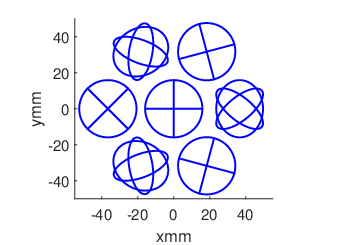
As outlined, magnetic induction is a useful propagation mechanism for medical in-body devices because of its capabilities in terms of power transfer and media penetration. In the following we study the performance and feasibility limits of magneto-inductive wireless powering (downlink) and data transmission (uplink) for micro-scale devices in the exemplary biomedical in-body application illustrated in Fig. 2. Thereby, the micro-scale in-body sensors are located beneath the skin and are each equipped with a multi-turn loop antenna (copper wire). The external device (above the skin) is both the data sink and the field source for wireless powering, for which it uses a transmit power of . The device features a massive array of 21 coils, each with circumference, in an arrangement that provides vast spatial diversity. We assume that are required for activation of the sensor chip (cf. reported in [14]) and that 50% of the excess received power is then used as transmit power in the uplink.

 |
 |
The system and coil parameters are chosen for best performance in this setting. The design frequency should be as large as possible for strong magnetic induction, cf. in (15), but sufficiently low to penetrate tissue and to not be limited by , i.e. the wavelength should exceed the coil wire length considerably. In that regard, we choose and single-turn coils with thick copper wire at the external device, which lead to better results than multi-turn coils. The coils have a Q-factor of and are treated as electrically small (the wavelength is ).
For the micro-scale sensors we assume single-layer solenoid coils whose height equals their diameter (henceforth called size) with turns and a turn spacing of wire diameters. We calculate their resistance with [10, Sec. 5.2.3], inductance with [15], and self-capacitance with [16, Eq. 5.3].
For simplicity, we make the idealistic assumptions of full channel state information (CSI) on both ends and full-duplex operation of down- and uplink. The chosen are close to the suggestion of by [17] and sufficiently low-frequency to penetrate a few of tissue. Thus, we can assume free-space propagation and still obtain meaningful implications for biomedical engineering, without a detailed model for tissue and body fluids (note that for water).
Each sensor node uses a two-port matching network of two lumped elements in L-structure. We assume that the generators of the high-complexity external device are not limited by their matching and, hence, we employ the transmit-side assumptions of (33) for the powering downlink. In the uplink, each coil of the external device (now receiving) has a two-port network for noise matching, implemented with a T-structure of three reactive lumped elements. The component values are optimized numerically for maximum average SNR (average in and over three orthogonal sensor orientations) at . We refrain from a full multiport matching network as it would be ultra narrowband and vulnerable to losses and drift due to the large number of lumped elements, e.g., in -structure. For the noise parameters we assume human body temperature for and (shielded environment), , LNA parameters per , and . We use the spatial correlation model with Bessel function .
V Numerical Results
V-A Single In-Body Sensor
We consider a single in-body sensor with arbitrary orientation and no passive relays. In the downlink, the external device transmits at the design frequency and uses maximum-ratio combining for beamforming to maximize the receive power. The resultant power transfer efficiency (PTE) is with channel vector . Fig. 3 shows the PTE over .


In the uplink, the sensor uses as transmit power if (otherwise, the sensor is in outage). The now receiving array performs maximum-ratio combining in every frequency bin based on the noise-whitened channel vector . The gains of the resultant parallel SISO channels are then used on the sensor side to find the spectral transmit power allocation with the waterfilling algorithm [18]. We study the uplink data rate in terms of the channel capacity .
Fig. 4 shows the evolution of uplink data rate over sensor-side coil size. We observe that a sensor can be activated and transmit data to outside the body if its coil is larger than . At this size, , and . Such size would be sufficiently small for many medical target applications [6]. With increasing size, the data rate grows rapidly as and the the mutual impedance to the external coils increase. Coils larger than about promise data rates beyond . The sensor orientation only has a weak impact on performance due to spatial diversity and the matching design of the array. Orientation-dependent signal attenuation is mitigated even further because reactive and radiative propagation modes are phase-shifted and both significant, because in (15). This is in contrary to the significant losses over unaligned near-field SISO links [19].
V-B Effect of Passive Relays
We investigate the effect of a randomly arranged swarm of 19 passive resonant relay coils around the sensor node. They could be placed in hopes of a performance gain or just represent nearby idle sensor nodes. Strong coupling to a relay detunes the sensor coil and shifts the resonance peaks in frequency, on the order of the sensor-coil bandwidth. Likewise, dense and arbitrarily arranged swarms of passive relays cause -selective channel fluctuations, i.e. fading [3]. We are interested in the implications for our application.
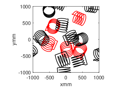
Henceforth we set the size of all sensor and relay coils to , resulting in , and . The passive relays are terminated with a capacitor for resonance at in uncoupled condition. All coil orientations are random with uniform distribution in 3D, see Fig. 2b, and the passive relay locations are sampled per coordinate from a Gaussian distribution about the sensor location (the standard deviation is 1.5 coil sizes and we resample until no coil geometries collide). We study the uplink rate with an elaborate scheme as well as a simple scheme: (i) adapt sensor matching to the coupling conditions, -tuning in the downlink and waterfilling in the uplink and (ii) no matching adaptation, downlink at the design frequency and flat uplink power allocation over the -bandwidth of the external coil.
Fig. 5a shows the resulting uplink rates for many realizations of the random swarm geometry. We observe that the relays indeed cause a fading effect. Clearly, meeting the -dependent fluctuations and detuning with appropriate measures improves the uplink; exploiting selective fading via transmit CSI is well-established for radio links [18]. Still, the presence of relays is detrimental in about 40% of cases.


V-C Cooperative Transmission with Other Sensors
Consider that the sensor node of interest is accompanied by other sensor nodes and possibly passive relays, and all activated sensors cooperate in the uplink. We assume that the sensors can establish phase synchronization because of the sub- operation. Furthermore, due to the strong links between neighboring sensors, we assume that their data exchange rates do not pose a bottleneck and thus the data rate of the cooperative uplink is determined by the final-hop rate. We assume the presence of 15 passive relays. All relay and sensor locations and orientations are sampled as described in Sec. V-B and an example arrangement is shown in Fig. 2b.
In the downlink, we use maximum-ratio transmit combining at the external array to maximize the received sum power over this MIMO channel, although subject to to activate the sensor of interest whenever possible. This way, vast power is fed to sensors with a good channel, with the idea that those sensors should see a good channel in the uplink, which depends on array matching and noise statistics though.
Again, we compare a simple scheme with no matching adaptation, downlink operation at and simplistic uplink power allocation (as in Sec. V-B) to a more sophisticated scheme which adapts the matching of the sensors to the coupling conditions and the signaling to the frequency-selective channel. For the latter, spectral power allocation in the uplink is concerned with per sensor . Since this case has no known analytical solution for the rate-optimal allocation [20] we choose a heuristic approach: each sensor allocates via waterfilling over the hypothetical parallel SISO channels that would arise when all other sensors are silent (but present) and the receive combining is as in Sec. V-A. We obtain an achievable uplink rate of where is found by solving the optimization problem subject to and the per-node power constraints given by the , which are incorporated according to Sec. II-F. Thereby, is the noise-whitened channel matrix in frequency bin .
Fig. 5b shows that the considered cooperative scheme yields a three- to fourfold increase of uplink data rate over the non-cooperative case in Fig. 5a, with the same amount of source power. Node cooperation can exploit the location-dependency of swarm-induced signal fluctuations, which usually improve the channel only for a subset of the nodes. Furthermore, the difference between the simplistic and elaborate approach is now more pronounced: in about 93% of cases, the elaborate scheme manages to utilize the passive relaying effect for a (sometimes significant) performance gain by exploiting the spectral and spatial channel variations.
VI Summary
We presented a general system model for magneto-inductive networks in order to study the performance limits of medical microsensors which receive power and transmit data via magnetic induction. For distance to the power source and data sink, the determined minimum coil size (copper wire) is about , while already allow for uplink data rate. We furthermore showed that the passive relaying effect in dense swarms of resonant nodes can be utilized for performance gains with adaptive matching, spectral power allocation, and/or node cooperation. Future research should extend the study to health regulations and propagation effects in tissue, absence of CSI, advanced materials (e.g. graphene) and compare to acoustic and optical approaches.
Appendix: In- and Output Impedance Matrices
When all inputs are terminated as shown in Fig. 1, the impedance matrices at the output ports are
| (34) | ||||
| (35) | ||||
| (36) |
With terminated outputs, the input impedance matrices are
| (37) | ||||
| (38) | ||||
| (39) |
References
- [1] K. Agarwal, R. Jegadeesan, Y.-X. Guo, and N. V. Thakor, “Wireless power transfer strategies for implantable bioelectronics,” IEEE Reviews in Biomedical Engineering, vol. 10, pp. 136–161, 2017.
- [2] S. Kisseleff, I. Akyildiz, and W. Gerstacker, “Digital signal transmission in magnetic induction based wireless underground sensor networks,” IEEE Transactions on Communications, vol. 63, no. 6, 2015.
- [3] G. Dumphart, E. Slottke, and A. Wittneben, “Magneto-inductive passive relaying in arbitrarily arranged networks,” in IEEE International Conference on Communications (ICC), May 2017.
- [4] E. Slottke, “Inductively coupled microsensor networks,” Ph.D. dissertation, ETH Zürich, 2016.
- [5] M. Sitti, H. Ceylan, W. Hu, J. Giltinan, M. Turan, S. Yim, and E. Diller, “Biomedical applications of untethered mobile milli/microrobots,” Proceedings of the IEEE, vol. 103, no. 2, pp. 205–224, 2015.
- [6] B. J. Nelson, I. K. Kaliakatsos, and J. J. Abbott, “Microrobots for minimally invasive medicine,” Annual Review of Biomedical Engineering, vol. 12, pp. 55–85, 2010.
- [7] B. Gulbahar, “Theoretical analysis of magneto-inductive THz wireless communications and power transfer with multi-layer graphene nano-coils,” IEEE Transactions on Molecular, Biological and Multi-Scale Communications, vol. 3, no. 1, pp. 60–70, 2017.
- [8] A. Servant, F. Qiu, M. Mazza, K. Kostarelos, and B. J. Nelson, “Controlled in vivo swimming of a swarm of bacteria-like microrobotic flagella,” Advanced Materials, vol. 27, no. 19, pp. 2981–2988, 2015.
- [9] M. T. Ivrlac and J. A. Nossek, “Toward a circuit theory of communication,” IEEE Transactions on Circuits and Systems I: Regular Papers, vol. 57, no. 7, pp. 1663–1683, 2010.
- [10] C. A. Balanis, Antenna Theory: Analysis and Design. Wiley, 2016.
- [11] Y. Hassan and A. Wittneben, “Adaptive uncoupled matching network design for compact MIMO systems with MMSE receiver,” in IEEE Wireless Communications and Networking Conference (WCNC), 2015.
- [12] Recommendation ITU-R P.372-13 Radio noise, Geneva, Sep 2016.
- [13] D. Nie, B. M. Hochwald, and E. Stauffer, “Systematic design of large-scale multiport decoupling networks,” IEEE Transactions on Circuits and Systems I: Regular Papers, vol. 61, no. 7, pp. 2172–2181, 2014.
- [14] X. Zou, X. Xu, L. Yao, and Y. Lian, “A 1-V 450-nW fully integrated programmable biomedical sensor interface chip,” IEEE Journal of Solid-State Circuits, vol. 44, no. 4, pp. 1067–1077, 2009.
- [15] H. C. Miller, “Inductance formula for a single-layer circular coil,” Proceedings of the IEEE, vol. 75, no. 2, pp. 256–257, 1987.
- [16] D. W. Knight, “The self-resonance and self-capacitance of solenoid coils,” 2016, DOI: 10.13140/RG.2.1.1472.0887. [Online]. Available: http://g3ynh.info/zdocs/magnetics/appendix/self-res
- [17] A. S. Poon, S. O’Driscoll, and T. H. Meng, “Optimal frequency for wireless power transmission into dispersive tissue,” IEEE Transactions on Antennas and Propagation, vol. 58, no. 5, pp. 1739–1750, 2010.
- [18] D. Tse and P. Viswanath, Fundamentals of Wireless Communication. Cambridge University Press, 2005.
- [19] G. Dumphart and A. Wittneben, “Stochastic misalignment model for magneto-inductive SISO and MIMO links,” in IEEE PIMRC, 2016.
- [20] S. Goguri, R. Mudumbai, D. R. Brown, S. Dasgupta, and U. Madhow, “Capacity maximization for distributed broadband beamforming,” in 2016 IEEE International Conference on Acoustics, Speech and Signal Processing (ICASSP). IEEE, 2016, pp. 3441–3445.