A physics-aware, probabilistic machine learning framework for coarse-graining high-dimensional systems in the Small Data regime
Abstract
The automated construction of coarse-grained models represents a pivotal component in computer simulation of physical systems and is a key enabler in various analysis and design tasks related to uncertainty quantification. Pertinent methods are severely inhibited by the high-dimension of the parametric input and the limited number of training input/output pairs that can be generated when computationally demanding forward models are considered. Such cases are frequently encountered in the modeling of random heterogeneous media where the scale of the microstructure necessitates the use of high-dimensional random vectors and very fine discretizations of the governing equations. The present paper proposes a probabilistic Machine Learning framework that is capable of operating in the presence of Small Data by exploiting aspects of the physical structure of the problem as well as contextual knowledge. As a result, it can perform comparably well under extrapolative conditions. It unifies the tasks of dimensionality and model-order reduction through an encoder-decoder scheme that simultaneously identifies a sparse set of salient lower-dimensional microstructural features and calibrates an inexpensive, coarse-grained model which is predictive of the output. Information loss is accounted for and quantified in the form of probabilistic predictive estimates. The learning engine is based on Stochastic Variational Inference. We demonstrate how the variational objectives can be used not only to train the coarse-grained model, but also to suggest refinements that lead to improved predictions.
†† Source code as well as examples can be found at: github.com/congriUQ/physics_aware_surrogateKeywords: Uncertainty Quantification, Bayesian Inference, Coarse-Graining, Variational Inference, Random Media, Multi-Physics Models
1 Introduction
The present paper is concerned with the data-driven construction of coarse-grained descriptions and predictive surrogate models in the context of random heterogeneous materials. This is of paramount importance for carrying out various uncertainty quantification (UQ) tasks, both in terms of forward and backward uncertainty propagation. More generally, the development of efficient surrogates is instrumental in enabling many-query applications in the presence of complex models of physical and engineering systems. The significant progress that has been materialized in the fields of statistical or machine learning Ghahramani 2015 in the last few years, particularly in the context of Deep Learning LeCun et al. 2015; Goodfellow et al. 2016 has found its way in physical systems where training data for the surrogates are generated by forward simulations of the reference, high-fidelity model. We note however that such problems exhibit (at least) two critical differences as compared to typical machine learning applications. Firstly, the dimension of the (random) inputs and outputs encountered in complex physical models is generally much larger than speech- or image-related data and associated tasks. Furthermore, the dependencies between these two sets of variables cannot be discovered with brute-force dimensionality reduction techniques. Secondly and most importantly, these are not Big Data problems. The abundance of data that can be rightfully assumed in many data-driven contexts, is contrary to the nature of the problem we are trying to address, that is learning surrogate models, or more generally enabling UQ tasks, with the least possible high-fidelity output data. Such regimes could be more appropriately be referred to as Small Data or better yet Tall Data in consideration of the dimensionality above Koutsourelakis et al. 2016.
The development of surrogates for UQ purposes in the context of continuum thermodynamics where pertinent models are based on PDEs and ODEs has a long history and some of the most well-studied methods have been based on (generalized) Polynomial Chaos expansions (gPC) Wiener 1938, Ghanem and Spanos 1991, Xiu and Karniadakis 2002 which have become popular in the last decade also due to the emergence of non-intrusive, sparse-grid stochastic collocation approaches Xiu and Hesthaven 2005; Ma and Zabaras 2009; Lin and Tartakovsky 2009. Despite recent progress in connecting gPC with domain decomposition methods Lin et al. 2010; Tipireddy et al. 2017; Tipireddy et al. 2018, these approaches typically struggle in problems with high-dimensional stochastic input, as is the case with random heterogeneous materials Torquato and Lu 1993 encountered in problems such as flow through porous media Bilionis et al. 2013; Atkinson and Zabaras 2019; Mo et al. 2018 or electromagnetic wave propagation through random permittivity fields Chauvière et al. 2006.
Another well-established strategy makes use of statistical couplings between the reference model and less expensive, lower-fidelity models in order to enable multi-fidelity methods O’Hagan and Kennedy 2000. In the context of PDEs, such lower-fidelity or reduced-order models may readily be constructed by utilizing potentially much coarser spatio-temporal discretizations which, in conjunction with appropriate statistical models, are capable of providing fully probabilistic predictions Koutsourelakis 2009; Perdikaris et al. 2017. The most striking benefit of such methods is that they automatically retain some of the underlying physics of the high-fidelity model and are therefore able to produce accurate predictions even when the data is scarce and the stochastic input dimensionality is high. Another category of algorithms falling under the class of reduced-order models is given by reduced-basis (RB) methods Hesthaven et al. 2016; Quarteroni et al. 2016 where, based on a small set of ‘snapshots’ i.e. forward model evaluations, the solution space dimensionality is reduced by projection onto the principal ‘snapshot’ directions. The reduced-order solution coefficients are then found either by standard Galerkin projection Rowley et al. 2004; Cui et al. 2015; Afkham and Hesthaven 2017 or regression-based strategies Yu and Hesthaven 2018; Guo and Hesthaven 2018; Hesthaven and Ubbiali 2018. Apart from issues of efficiency and stability, both gPC and RB approaches in their standard form are generally treated in a non-Bayesian way and therefore only yield point estimates instead of full predictive posterior distributions.
A more recent trend is to view surrogate modeling as a supervised learning problem that can be handled by pertinent statistical learning tools, e.g. Gaussian Process (GP) regression Rasmussen and Williams 2006; Bilionis and Zabaras 2017 which provide closed-form predictive distributions by default. Although recent advances have been made towards multi-fidelity data fusion O’Hagan and Kennedy 2000; Raissi et al. 2017; Perdikaris et al. 2015 and incorporation of background physics Raissi and Karniadakis 2018; Yang et al. 2018; Lee et al. 2018; Tipireddy and Tartakovsky 2018 via Gaussian Processes, the poor scaling behavior with stochastic input dimension remains one of the main challenges for GP models.
More recently, deep neural networks (DNNs) LeCun et al. 2015; Goodfellow et al. 2016 have found their way into surrogate modeling of complex computer codes Tripathy and Bilionis 2018; Zhu and Zabaras 2018; Mo et al. 2018; Yang and Perdikaris 2019. One of the most promising developments in the integration of such tools in physical modeling are physics-informed neural networks Raissi et al. 2017; Raissi et al. 2019; Tartakovsky et al. 2018 which are trained by minimization of a loss function augmented by the residuals of the governing equations Raissi et al. 2017 and Raissi et al. 2017. In Zhu et al. 2019, this methodology is generalized and extended to cases without any labeled data, i.e. without computing the output of the reference, high-fidelity model. However, such models transfer much of the numerical burden from the generation of training data to the repeated evaluation of the residual during model training. While promising results have been obtained, we note that several challenges remain with regards to the incorporation of prior physical knowledge in the form of symmetries/invariances etc. into DNNs as well as their capabilities under extrapolative conditions.
In this paper, we present a novel, fully Bayesian strategy for surrogate modeling designed for problems characterized by
- •
high input dimension, i.e. the “curse of dimensionality” – in the problems examined, we consider input data (random material microstructures) of effective dimensionality ; and
- •
small number of training data , i.e. forward or fine grained model (FGM) input/output pairs that can practicably be generated in order to train any sort of reduced-order model or surrogate – in the examples presented here, we use training samples.
In the context of random media and in order to achieve the aforementioned objectives, it is of primary importance (a) to extract only the microstructural features pertinent for reconstruction of the fine-grained model (FGM) output and (b) to construct a surrogate that retains as much as possible the underlying physics of the problem. Whilst point (a) should effectively reduce the input dimension, (b) may exclude a myriad of potential model outputs violating essential physical principles of the FGM. Consequently, the core unit of the surrogate model established here is based on a coarse-grained model (CGM) operating on simplified physics valid on a larger scale than the characteristic length of the microstructural features in the FGM. The CGM serves as a stencil that automatically retains the primary physical characteristics of the FGM. It is parametrized by a latent, low-dimensional set of variables that locally encode the effective material properties of the underlying random heterogeneous microstructure and are found by appropriate sparsity-inducing statistical learning Schöberl et al. 2017. Finally, a decoder distribution maps the CGM outputs to the FGM solution space, yielding fully probabilistic model predictions. Instead of viewing the encoding step (dimension reduction) separately from the surrogate modeling task Ma and Zabaras 2011; Xing et al. 2016, both are integrated and trained simultaneously, ensuring that the encoded, latent representation of the microstructure is maximally predictive of the sought FGM response instead of the original fine-scale microstructure itself. Model training is carried out using modern Stochastic Variational Inference (SVI) techniques Paisley et al. 2012; Hoffman et al. 2013 in combination with efficient stochastic optimization algorithms Kingma and Ba 2014. A hierarchical Bayesian treatment of the model parameters obviates any need for fine-tuning or additional input by the analyst Bishop and Tipping 2000.
The rest of the paper is organized as follows. Section 2 lays the methodological foundations for the proposed model, including a presentation of the pertinent physical structure, associated state variables and governing equations. Moreover, a detailed definition of both encoding and decoding steps is given, as well as a clear specification of the prior model and the training/prediction algorithms. In section 3, we provide numerical evidence that the proposed model can lead to accurate predictions even when trained on a few tens of FGM data. Furthermore, we present a methodological framework for adaptively adjusting the CGM complexity in order to enhance its predictive ability. Section 4 summarizes the main findings and presents further extensions and possible applications of the proposed model.
2 Methodology
We present a general, probabilistic framework to coarse-graining which we specialize in the subsequent sections. The starting point is an expensive, deterministic, fine-grained model (FGM) with high-dimensional, random inputs and high-dimensional outputs . Due to the high dimensionality of the input uncertainties and the small number of forward evaluations that can practically be performed, any naive regression approach, i.e. learning a direct map from to is doomed to fail.
We seek instead a lower-dimensional, effective representation of the high-dimensional stochastic inputs which encodes as much as possible information on the respective FGM output , see Figure 1. We note that this differs from classical dimension reduction approaches in the sense that the encoded representation should be maximally predictive of the FGM output – and not for the reconstruction of itself Tishby et al. 1999. Rather than assigning an abstract, statistical meaning to , we associate them with a less-expensive, physical, coarse-grained model (CGM). In particular, the latent variables represent the inputs of the CGM. We denote by the corresponding CGM outputs which we subsequently attempt to link with the FGM response , see Figure 1. The CGM effectively represents the bottleneck through which information that the FGM input provides about the FGM output is squeezed. While several possibilities exist, independently of the final choice for the CGM, information loss will generally take place during the coarse-graining process, which in turn results in predictive uncertainty that we aim at quantifying. Moreover, tools for comparing different CGMs as well as strategies of refining the CGM adaptively in order to improve predictive accuracy are developed in a later section.

The general framework described above can be effected by a model that integrates the following three key components (see Figure 1 and Grigo and Koutsourelakis 2017; Grigo and Koutsourelakis 2019):
- •
Encoding - Dimension reduction: A mapping from the high - dimensional microstructural description to a much lower-dimensional quantity retaining as much as possible information on the corresponding response – this mapping is carried out probabilistically by the conditional distribution parametrized by .
- •
Model reduction: A skeleton of a coarse-grained model (CGM) that employs the dimension-reduced quantities as input and yields an output . Such a model can be based on simplified physics and/or coarser spatial discretization. In our case, this is constructed by employing a coarse discretization of the Darcy-flow governing equations as it will be explained in detail later. We denote by the generally stochastic input-output map implied.
- •
Decoding - Reconstruction: A probabilistic mapping from the CGM output back onto the original FGM output – this mapping is mediated by the distribution parametrized by .
The combination of the aforementioned three densities yields
| (1) |
Assuming a deterministic CGM, i.e. , this simplifies to
| (2) |
The resulting parametrized density can be viewed as the likelihood of a FGM input/output pair and is thus the key quantity in the proposed probabilistic surrogate. We note that the three constitutive densities are highly modular and can be adapted to the particulars of the FGM and the CGM adopted. In the following, the FGM consists of a Stokes-flow simulator through a random heterogeneous medium, see section 2.1. The CGM is described by Darcy’s equations of flow through a permeable medium and is explained in section 2.2. We present the essential components of the proposed model as well as the specialization of the variables and densities above in section 2.3. In section 2.4, we present the learning engine that is capable of training the model with small data and in section 2.5, we discuss how the trained model can be used to produce probabilistic predictions. We conclude this methodological section with a discussion on the numerical complexity (section 2.6) as well as a novel algorithm for the adaptive refinement of the coarse-grained model (section 2.7).
2.1 The fine-grained model: Stokes flow through random porous media

Flow of incompressible Newtonian fluids through random porous media is characterized by low fluid velocities and is therefore dominated by viscous forces. In such regimes, the steady-state Navier-Stokes equations reduce to Stokes equations of momentum and mass conservation,
| (3a) | ||||||
| (3b) | ||||||
where and are pressure and velocity fields, is an external force field, the pore part of the domain , where denotes the part of impermeable solid material, and the fluid viscosity which we may set to for convenience.
On the solid-fluid interface , the no-slip boundary condition
| (3c) | ||||||
is imposed, whereas on the boundary of the macroscopic system, we apply
| (3d) | ||||||
| (3e) | ||||||
where is the Cauchy traction and the unit outward normal.
For the remainder of the paper, we consider a unit square domain with randomly distributed non-overlapping polydisperse spherical exclusions, see Figure 2 for a schematic representation. Such microstructures exhibit topologically fully connected pore spaces and lead to unique solutions of (3) for the case where .
For the numerical solution of Equation (3), we employ triangular meshes with standard Taylor-Hood elements (i.e. quadratic and linear shape functions for velocity and pressure, respectively), implemented using the FEniCS finite element software package Logg et al. 2012. For generic two-phase media, consists of a list of binary variables representing the phase of each pixel/voxel. For the particular case considered of randomly distributed non-overlapping polydisperse spherical exclusions, one could also represent the microstructure with a list of exclusion center coordinates and the corresponding radii. We denote by the discretized solution vector which can consist of pressures or velocities and write
| (4) |
to indicate the map from the microstructure to the PDE response of interest.
Computational considerations
Typically, the structure of the porous material is very complex with a characteristic length-scale much smaller than the macroscopic length scale of the problem domain . This large difference in scales means that (a) from a modeling point of view, a probabilistic description would be more realistic for the porous microstructure, and (b) the numerical solution of (3) requires discretizations fine enough to resolve all microstructural details. Moreover, the uncertainty of microstructures requires repeated evaluation of the numerical solver (4) to obtain accurate estimates (e.g. with Monte Carlo) of any statistic of interest relating to the output which quickly becomes impracticable due to the significant cost associated with each FGM run.
2.2 The coarse-grained model: Darcy equations for diffusion through a permeable medium
The macroscopic Darcy-like behavior of Stokes flow through random porous media (3) is a long-standing result from homogenization theory first shown for periodic microstructures Sanchez-Palencia 1980; Tartar 1980, later generalized for connected solid phase matrix Allaire 1989, the non-stationary process Allaire 1992 and non-periodic media Whitaker 1986. In classical homogenization, the crucial step is to find a local boundary value problem on a Representative Volume Element (RVE) Sandström et al. 2013; Marchenko and Khruslov 2006; Tartar 2010. The RVE size , i.e. the radius of the averaging volume, must be large compared to the microstructural length scales . On the other hand, the volume averaged quantities, i.e. the intrinsic phase averages and , should show sufficient variation over the problem domain , i.e. should be large compared to . To summarize, Stokes to Darcy convergence is observed in the limit of
| (5) |
which, according to Whitaker 1986, may slightly be relaxed to the conditions
| (6) |
to safely assume Darcy-type flow. Using the definition for the intrinsic phase averages of pressure and velocity fields and
| (7) |
where is the volume of the fluid part of the RVE, the effective Darcy constitutive behavior can be written as
| (8a) | ||||||
| (8b) | ||||||
| (8c) | ||||||
| (8d) | ||||||
with the unit outward normal vector , the viscosity and some unknown permeability tensor . Determining/estimating the effective permeability field remains a substantial computational problem which in homogenization theory is usually approached by solving an RVE subscale problem Sandström et al. 2013. We emphasize that full Stokes/Darcy equivalence can only be assumed in the limit of infinite scale separation as defined by Equation (5). However, this does not rule out the possibility to use the Darcy equations as a stencil of a machine learning model applied to fine-grained Stokes flow data even far away from the scale separation limit, as we will see in the experiments section 3.
2.2.1 The Darcy permeability tensor field
The material parameters of the CGM which provide the necessary closure pertain to the permeability tensor field . We subdivide the problem domain into of non-overlapping subregions/ cells such that and for . In most cases examined in the experimental section 3, the subregions are squares of equal size, as can be seen in the bottom row of Figure 11. Within each subregion , a constant permeability tensor is assumed, i.e.
| (9) |
where is the indicator function of subregion . The local permeability tensors are positive definite matrices which, in the simplest case based on the isotropy assumption, take the form
| (10) |
where is the identity matrix. We note that the number of cells does not need to coincide with the finite elements employed for the solution of the CGM. The former control the dimension of the reduced representation whereas the latter determine the computational cost in the solution of the CGM. Naturally, different discretizations or representations of the coarse model’s spatially-varying properties can be adopted, e.g. could relate to basis functions’ coefficients in an appropriate expansion of .
Analogously to the FGM in Equation (4), the Darcy-based, coarse-grained model (CGM) is defined as the deterministic mapping
| (11) |
Remarks
- •
The low-dimensional latent variables encode the high dimensional descriptors of the fine scale porous domain of the Stokes flow FGM as an effective, Darcy-type permeability random field . We re-emphasize that it is extraneous if the latent representation is a faithful decoding of its fine scale analogue for the purpose of accurately reconstructing directly. Instead, must be maximally predictive (when solving the inexpensive CGM ) of the reconstruction of the FGM output . Hence, may be completely different from the reduced coordinates identified by typical dimensionality reduction techniques applied directly on . The encoder density should therefore be trained in such a way that it extracts all microstructural features from that are relevant in predicting the FGM output .
- •
The decoder density attempts to reconstruct the FGM Stokes flow response given the solution of the Darcy-based CGM Equation (8). While a general parametrization can be employed (e.g. making use of (deep) neural networks), this would necessitate either huge amounts of data or very strong regularization assumptions. We exploit instead the spatial character of the problem, i.e. if the FGM and CGM outputs are directly related to spatial locations (e.g. if they represent pressure or velocity responses at these points), it is natural to assume that components corresponding to points in the vicinity of are most relevant for reconstruction of corresponding to point .
- •
Independently of the values assigned to the parameters , predictions produced by the surrogate will be probabilistic as reflected by the density in Equation (2). This can be attributed to the epistemic uncertainty due to the unavoidable information loss during the coarse-graining process as there is an upper bound on the mutual information when and no redundancies in Tishby et al. 1999.
The following subsections are devoted to giving a clear description of the main building blocks and as well as of the prior model we apply on the model parameters and .
2.3 Components of the proposed model
2.3.1 The encoder distribution
The encoder distribution that effects the mapping from the high-dimensional to the lower-dimensional can assume various forms. Any successful strategy should be capable of extracting appropriate features from or, more generally, learning the right representation for predicting . An obvious choice would be to exploit the expressive power of (deep) Neural Nets (NNs) and, given the spatial character of , Convolutional Neural Networks (CNNs) in particular Fukushima 1980; Lecun et al. 1998; Krizhevsky et al. 2012. A common misconception is that Deep Learning techniques are devoid of any feature engineering. While deep NNs are highly expressive, contain a lot of learnable parameters and reduce the need for feature engineering, it is not true that data pre-processing or feature extraction are totally irrelevant22 2 https://github.com/tensorflow/transform. Several components, such as the number, size and type of layers or e.g. the type and number of pooling layers in CNNs are in fact hard-coded, feature-extraction mechanisms. More importantly, the basic premise in successful applications of these models is the availability of large amounts of data, from which the necessary information can be extracted. As mentioned earlier however, we operate in the Small Data regime.
Based on this, we make use of a large set of physically-motivated, feature functions (discussed in detail in the sequel) in the context of the following model:
| (12) |
In principle, the type and number of features can differ with every latent space component . These feature functions are linearly combined with coefficients (potentially different for every component as well) and augmented with residual Gaussian white noise of variance , so that the set of free parameters for the distribution is 33 3 We use the notation , where is the vector of variances, wherever it is more convenient..
The distribution for is thus
| (13) |
with being the vector of feature functions used to predict the latent space component .
Feature functions:

The most critical aspect in the expressivity of the encoder pertains to the feature functions employed. In this work, we make use of morphological measures Torquato 2001; Lu and Torquato 1992; Torquato and Lu 1993; Lowell et al. 2006, quantities from classical fluid dynamics Sutera and Skalak 1993; Kozeny 1927; Carman 1937 or other physics Archie 1947, image analysis Soille 1999 and low-dimensional autoencoder representations Doersch 2016. Some important classes of possible feature functions are depicted in Figure 3 and briefly explained in the following list:
- •
Pore fraction: The fraction of pore space over a certain region and several nonlinear functions thereof (e.g. certain powers);
- •
Interface area: The interface area between matrix- and exclusion phase over a certain region and nonlinear functions thereof;
- •
Effective medium approximations: There exist several approximation formula for effective material properties in diffusion problems (Bruggeman formula Bruggeman 1935, Maxwell-Garnett approximation Landauer 1978) which can be generalized to the infinite contrast limit of matrix/exclusion phase permeabilities;
- •
Chord length density: The density of lengths of segments of an infinitely long line being in either matrix or exclusion phase, see blue line with red dots in Figure 3. A ‘segment’ is a part of the line between two neighboring dots – the feature function is given by evaluating the chord length density for several lengths , see 3 for the length scales used in the experiments;
- •
Statistics of exclusion radii: Mean, variance, max, min, etc. of exclusion radii;
- •
Statistics of mutual exclusion distances: Mean, variance, max, min, etc. of mutual exclusion distances (center-to-center or edge-to-edge). See the orange lines in Figure 3 for illustration;
- •
Pore-size density: Density of the distance from a random point in to the nearest matrix/exclusion interface. For illustration see the red/gray circles in Figure 3. Nearest-neighbor functions Torquato 2001 are closely related. Again, the pore-size density is to be evaluated for several lengths , see 3;
- •
- •
2-point correlations: The probability, that two random points of distance lie both in matrix (exclusion) phase – see 3 for lengths ;
- •
Distance transforms: For any point in , compute the distance to the closest exclusion (matrix phase), see right part of Figure 3. Features can be constructed from statistics of the distance transform.
Ultimately, several hundreds of such functions can be deployed – in Section 3, we use the 150 listed in Table 3. In order to avoid overfitting in the Small Data regime we are operating (i.e. ), we make use of a fully Bayesian, sparsity-inducing prior model Bishop and Tipping 2000 capable of automatically controlling model complexity by pruning all irrelevant features and identifying the most salient ones, see section 2.3.3.
2.3.2 The decoder distribution
The probabilistic coarse-to-fine mapping should take into account the spatial characteristics of the problem, e.g. that FGM and CGM outputs may be given by physical quantities evaluated at spatial locations . For simplicity, let us assume that is the pressure field solution of the FGM Equation (3) interpolated at a regular fine scale grid , , and its Darcy counterpart from Equation (8) evaluated at a much coarser grid , . Then the model for could look like
| (14) |
where should have the structure of an interpolation matrix from to and is a diagonal precision matrix to be learned from the data. The decoder distribution can thus be written as
| (15) |
with model parameters . We emphasize that many different possibilities exist in terms of the parametrization and architecture of . One should note here that, in contrast to which involves a map from the high-dimensional to a lower-dimensional , encompasses a map from the lower-dimensional to the high-dimensional which is obviously much more manageable. As with , the option of NNs comes to mind and given the spatial character of both and CNNs could be introduced. We have again decided against this option, due to the Small Data setting of the problem. Given the lower dimension of the inputs , nonlinear models employing polynomials, kernels etc could be employed. An interesting alternative involves Bayesian non-parametric extensions. For instance, a Gaussian Process regression could be deployed for the probabilistic mapping , exploiting the spatial structure of the problem by making use of a stationary covariance kernel of the form . Alternatively, each can be expressed using an independent Gaussian Process in a fashion analogous to GP-LVMs Lawrence 2005; Titsias and Lawrence 2010. Such an extension is not pursued here due to the complexities associated with the inference and prediction steps Damianou et al. 2015.
2.3.3 The prior model
We advocate a fully Bayesian formulation where the (approximate) posterior densities on the model parameters may be computed. In view of the Small Data setting, we employ priors that can safeguard against overfitting, that do not require any fine-tuning or have ad hoc hyperparameters, but also promote interpretability of the results. To that end, in order to induce sparsity in the feature functions of given in Equation (13), we make use of the Automatic Relevance Determination (ARD) model Faul 2003 corresponding to
| (16) |
where the precision hyperparameters are equipped with a conjugate Gamma hyperprior
| (17) |
This hierarchical model has been widely studied and the capability of pruning irrelevant parameters has been shown when small values for the hyperparameters are employed44 4 In our investigations, we set to avoid division by zero without affecting the converged values. Bishop and Tipping 2000; Tipping 2001.
Similarly, we apply conjugate, uninformative Gamma hyperpriors55 5 See footnote 4 on the precision parameters in the encoder/decoder distributions and , i.e.
| (18) | ||||
| (19) |
A vague, uninformative prior could also be used for but as this was found to have no measurable effect on the results and in order to lighten the notation, we completely omit it.
2.4 Model training
The probabilistic graphical model described thus far is depicted in Figure 4. Given a dataset consisting of FGM input/output pairs (i.e. Stokes-flow model simulations) , the model likelihood can be written as (see Equation (2))
| (20) |
where is a diagonal precision matrix and are the latent variables that encode the coarse-grained material properties for each sample . Given the aforementioned priors, the posterior of the model parameters is
| (21) |
where . The posterior over all variables is given by
| (22) |
where is the model evidence of the postulated coarse-graining model Gelman et al. 2003. This is a pivotal quantity in model validation that as we show later will serve as the main driver for the refinement/enhancement of the CGM.
Evaluating the integrals in Equation (21) is analytically intractable, making necessary the use of suitable (approximate) inference methods that are capable of giving fast and accurate estimates of the above posterior. In this work, we employ Stochastic Variational Inference (SVI, Paisley et al. 2012; Hoffman et al. 2013) methods which produce closed-form approximations of the true posterior and simultaneously of the model evidence . In contrast to sampling-based procedures (e.g. MCMC, SMC), SVI yields biased estimates at the benefit of computational efficiency and computable convergence objectives in the form of the Kullback-Leibler (KL) divergence between the approximation and the true posterior Blei et al. 2017:
| (23) |
We note that the evidence can be decomposed as
| (24) |
where
| (25) |
Since , provides a rigorous lower bound to , called the evidence lower bound (ELBO). Hence minimizing is equivalent to maximizing the ELBO .
We employ a mean-field approximation to the full posterior based on the following decomposition:
| (26) |
If denotes an arbitrary subset of the parameters above (i.e. if is effectively one of the component variables ), then the optimal can be found by setting the first order variation of to zero yielding Beal and Ghahramani 2003
| (27) |
where denotes expectation w.r.t. all ’s except for . We emphasize that every implicitly depends on all other ’s, which means we need to self-consistently cycle over all and update given expected values w.r.t. all , until convergence is attained. We provide complete details of the derivations in A and summarize here the closed-form update equations
| (28) |
| (29) |
| (30) |
| (31) |
where denotes expected values w.r.t. as specified in (26). Due to the choice of conjugate priors, most expected values are given in closed form,
| (32) |
The optimal form of the remaining approximate posteriors, i.e. , is given by (based on Equation (27))
| (33) |
which is analytically intractable due to the expectations with respect to the output of the CGM (i.e. of the Darcy-flow simulator). Instead of approximating the expectations above by Monte Carlo, we retain the variational character of the algorithm by employing approximations to the optimal which take the form of multivariate Gaussians with a diagonal covariance, i.e.
| (34) |
and find the optimal values of the parameters via black-box variational inference Ranganath et al. 2014; Hoffman et al. 2013; Paisley et al. 2012, i.e. by minimizing the KL-divergence between and the optimal in Equation (33),
| (35) |
The computation of the objective above as well as gradients with respect to involves expectations of the CGM outputs as well as their respective gradients . The latter are efficiently computed using adjoint formulations (see e.g. Heinkenschloss 2008; Constantine et al. 2014). In order to minimize the noise in the expectations involved, we apply the the reparametrization trick Kingma and Welling 2013 and supply the stochastic gradients to the adaptive moment estimation optimizer (ADAM Kingma and Ba 2014). We note that this stochastic optimization problem needs to be run for every data point in every training iteration, but is entirely parallelizable in . After optimization, the expected values are readily given by the first and second moments of the resulting Gaussian specified in Equation (34), whereas the expected values can efficiently be obtained by direct Monte Carlo. Full details about the performed black-box VI are given in A.1. All steps of the training process are summarized in Algorithm 1.
2.5 Model predictions
A main feature of the coarse-grained model presented in this work is the capability to produce probabilistic predictions that quantify uncertainty both due to limited training data and due to limited model complexity, i.e. the information loss happening during the coarse-graining process going . In particular, given training data and a new FGM input (which is not included in the training data ), the predictive posterior density for the corresponding FGM output is
| (36) |
with the decoding/encoding distributions as described in sections 2.3.1, 2.3.2. We make use of the variational approximation (section 2.4) to the posterior
| (37) |
in order to rewrite the predictive posterior as
| (38) |
By drawing samples from the approximate posterior, the integration above can be performed efficiently with Monte Carlo since the cost of each sample is very small as it entails solely CGM output evaluations. We note though that some of the integrations involved in the computation of lower-order statistics can also be done (semi)-analytically. In particular, we note that the predictive posterior mean is given by:
| (39) |
where denotes the predictive posterior average of the CGM output computed with Monte Carlo by ancestral sampling. Similarly, one can compute the posterior predictive covariance of the FGM output vector , which we denote by , as
| (40) |
where denotes the predictive posterior covariance of the CGM output vector which can be estimated by Monte Carlo and correspond to the posterior averages of reciprocal precisions which can be computed in closed form based on Equation (30).
The computational steps to generate predictive samples from the generally non-Gaussian for an unseen microstructural input is summarized in Algorithm 2.
The training (offline) and prediction (online) stages are represented graphically in the workflow diagram in Figure 5.
2.5.1 Model performance metrics
Apart from computational efficiency, the key objective of any surrogate model is its predictive accuracy, i.e. its closeness to the true FGM solution . In order to assess this, we consider separate test datasets , where the are drawn from the same distribution that was used for the training set . We report metrics that reflect both the accuracy of point estimates of the predictive posterior (e.g. in Equation (39)) as well as the whole density (Equation (38)).
In particular, we compute the coefficient of determination Zhang 2017
| (41) |
where is the sample mean of the FGM output over the test dataset. The denominator normalizes the point deviation in the numerator by the actual variability of the true outputs. In the case of perfect prediction, , the second term in (41) vanishes and which is the largest value it can attain. Smaller values of indicate either larger deviation of the mean prediction from the truth or smaller variability in the components.
The second metric we employ is the mean log likelihood Zhu and Zabaras 2018 given by
| (42) |
We note that when degenerates to a discrete density centered at the true i.e. not only it predicts perfectly the FGM output but there is no predictive uncertainty, then the attains the highest possible value of . In the other extreme if for one or more of the test samples , at the true , then attains its lowest possible value of . Hence, attempts to measure the quality of the whole predictive posterior . Given that the integration in Equation (38) is analytically intractable and no closed-form expression for can be established, we evaluate under the assumption that can be adequately approximated by a multivariate Gaussian with mean (Equation (39)) and a diagonal covariance which consists of the diagonal entries of (Equation (40)) which we represent with the vector . In this case:
| (43) |
In the numerical experiments discussed in section 3, is used, leading to negligible Monte Carlo error due to variation of test samples.
2.6 Numerical complexity analysis
|
||||||||
| training |
| |||||||
| prediction |
For analysis of the numerical complexity of the proposed model, it is vital to distinguish between training (offline) and prediction (online) phases, see also Figure 5. There are basically six quantities that are relevant for the computational cost of both stages. These are the number of training data , the dimension of the FGM input , the dimension of the FGM output , the dimension of CGM input , the dimension of the CGM output and the number of feature functions per latent space variable .
As it can be seen in Algorithm 1, the complexity of the training stage depends linearly on the number of training data (for-loop), but is fully parallelizable over every data point. The prediction stage only sees the final (approximate) posterior , so that the scaling is independent of . Both training and prediction phases scale linearly with the fine scale output dimension , since they only involve vector operations. For the same reason, the scaling with respect to is linear. Scaling with depends on the CGM solver i.e. in the worst case, for the linear Darcy model with a direct solver, the scaling is . We apply a sparse banded solver, which scales as . Scaling with the dimension of microstructural inputs is dependent on the set of applied feature functions and ranges from (e.g. constant feature, i.e. ) to (e.g. mean mutual distance of circular exclusions). Finally, scaling with respect to is see Equation (31). Furthermore, in the prediction stage, it is possible to omit components of that have been pruned out by the applied sparsity prior, thereby avoiding the cost connected to the evaluation of corresponding feature functions. The scaling characteristics of training and prediction phases is summarized in table 1.
2.7 Automatic adaptive refinement
As already mentioned in section 2.4, the evidence lower bound (ELBO) is an approximation to the model’s evidence. The latter balances the model’s fit to the data with the model’s complexity and serves as a parsimonious metric of how well the model can explain the training data Murray and Ghahramani 2005; Rasmussen and Ghahramani 2001. This quantity can therefore be used not only for scoring different competing models which have been trained on the same data, but also as the objective to any refinement of an existing model. According to Equation (25), the ELBO is given by the expected value
| (44) |
where is given in Equation (22) and is the variational approximation to the posterior as defined in (26). Since all of the expected values needed in the right side of the above equation are estimated during model training, the ELBO can be evaluated explicitly and be used to also monitor convergence behavior during training. In order to keep this section uncluttered, the final expression for the ELBO is given in D.
While one can envision many ways of refining the coarse-grained model, we focus here on the latent variables . These constitute the bottleneck through which information that the FGM input provides about the FGM output is squeezed. Physically, they relate to the effective permeability of the Darcy-based CGM and assuming a model according to equations (9)–(10), they are inherently tied with the piecewise-constant discretization adopted, i.e. each component relates to the Darcy permeability in a square subregion of the problem domain.
The question we would like to address is the following: If one was to refine the piecewise-constant representation of the Darcy permeability field in equations (9)–(10) by subdividing one square cell of the existing partition into smaller subregions, then which would yield the best possible model? We note that such a refinement would lead to an increase in the dimension of the bottleneck variables which, in principle, should lead to more information form being retained.
Given a fixed refinement mechanism of an , say by subdividing into 4 equal squares (in two-dimensions), a brute force solution strategy would be to refine one of the existing at a time, train the new model, compute its ELBO and compare with the others. Obviously such a strategy is computationally cumbersome particularly when the number of existing subregions is high. The cost would be even greater if one was to consider all possible combinations of two or more subregions that could be refined at the same time.
We thus propose a procedure based on the decomposition of the ELBO into contributions from different subregions (and therefore ) according to , where with we denote terms that cannot be assigned to any of the subregions . As the goal is ultimately to increase the ELBO of the model, we propose selecting for refinement the cell with the lowest contribution and therefore contributes the least in explaining the data. This strategy is analogous to the one advocated in Ghahramani and Beal 2000 for refining components in a mixture of factor analyzers. Hence we use as the scoring function of each subregion/cell. The derivation of is contained in D. and we include here only the final expression which, for a model with tied , is
| (45) |
where is the posterior variance of (see equations (34) and (35)), are given in Equation (29) and is the posterior variance of the parameters given in Equation (31).
Keeping in mind that the subregion/cell with the smallest is proposed for refinement, the scoring function defined by Equation (45) favours cells where the posterior variances of the tend to be small, i.e. tight (approximate) posterior distribution , whereas at the same time, the expected decoder misfit (see Equation (29)) should be large but there should be high certainty about the feature coefficients , i.e. low . We finally note that once the cell with the lowest has been identified and split, training is restarted with all model parameters initialized to their previously converged values. We illustrate these steps by example in section 3.6.
3 Numerical examples
The numerical experiments carried out in this paper are aimed at replacing the expensive Stokes flow FE simulation defined by Equations (3)–(4) by an inexpensive, Bayesian, coarse-grained model built around the Darcy-flow skeleton as presented in sections 2.2–2.6. We begin this section with a clear specification of the FGM data generation and the model distributions . Subsequently, we show that close to the homogenization limit (i.e. infinite scale separation) defined by Equation (5), the proposed coarse-grained model is capable to accurately reconstruct the FGM solution by learning (from a small number of FGM training samples) the requisite effective properties without ever solving any of the equations homogenization theory describes. Thereafter, we investigate the coarse-grained model’s predictive quality as a function of the number of training data and the latent space dimensionality for microstructural data far from the homogenization limit (without scale separation). We show that the model indeed exhibits feature sparsity in learning the effective Darcy permeability field . We then apply the surrogate to an uncertainty propagation (UP) problem and finally demonstrate the performance of the proposed adaptive refinement objective and associated algorithm. Source code as well as examples can be found at: https://github.com/congriUQ/physics_aware_surrogate
3.1 Experimental setup
3.1.1 Fine scale microstructural data

Throughout the following experiments, we use randomly distributed, non - overlapping polydisperse spherical exclusions from a unit square domain as depicted in Figure 2. The total number of exclusions of a material sample as well as the radii , are sampled from a log-normal distribution,
| (46) | ||||
| (47) |
The coordinates of the center of each exclusion are drawn from a Gaussian process with squared exponential kernel of length scale warped with the logistic sigmoid function ,
| (48) |
where and a squared exponential covariance
66
6
Note that the resulting distribution is distorted by the fact that a sampled exclusion is rejected if it overlaps with an exclusion which has been inserted before.. Also, the (location-dependent) -normal mean of exclusion radii is drawn from a Gaussian process for every sample according to
| (49) |
with the corresponding covariance kernel. Four microstructural samples generated according to the described distributions are depicted in Figure 6. After generation of a microstructure, the domain is pixelized into a grid of size . The corresponding binary vector representing the phase of each pixel makes up the FGM input , i.e.:
| (50) |
The sampled microstructres are passed to the FEniCS mshr Logg et al. 2012 module to generate a triangular finite element mesh containing roughly vertices. The output of interest, i.e. , consists of the the interpolated pressure values on a regular grid of i.e.:
| (51) |
Depending on the total number of exclusions , generation of a single mesh takes in between hours (for ) up to 10 days (for ) of computation time on a single Intel Xeon E5-2620 (2.00 GHz) CPU. The average solution for each FGM (i.e. Stokes-flow) PDE-solve takes 1512s 5.7s on the same hardware.
We use boundary conditions on the FGM pressure and velocity fields of the form
| (52) |
where denotes the origin of the domain, i.e. the point . The boundary condition coefficients and may assume different values in the following experiments and are therefore specified later.
3.1.2 The CGM
For the Darcy-type reduced order model , we use a finite-element solver to Equations (8) as described in section 2.2, operating on a regular square grid endowed with bilinear shape functions. The coarse-grained random permeability field of the CGM Darcy solver is assumed to have the form defined by equations (9)–(10) throughout this section.
3.1.3 The encoder distribution
For the encoder distribution , we assume a model as defined by equations (12)–(13), with the restriction that
| (53) |
where denotes the subset of the microstructure which corresponds to the permeability field cell . Equation (53) essentially states that the same set of features are used for every permeability field cell , where denote features evaluated on the global domain and on a local cell permeability field cell , respectively. It is noted though that the coefficients are generally different for different cells . A Table of all feature functions used in the experiments is given in B.
Prior on
The prior defined in Equation (16) is restricted such that the precision hyperparameters , i.e. all permeability field cells share the same set of hyperparameters . This leads to the same set of activated features, i.e. features with nonzero, but generally different for different cells , such that permeability cells are enabled to share information across the whole domain .
3.1.4 The decoder distribution
The decoder distribution we use in the experiments is defined by equations (14)–(15). As the FGM model output , we choose to use the Stokes flow pressure response linearly interpolated onto a square rectangular grid in the unit square domain . Although parameter uncertainty on the coarse-to-fine projection matrix could readily be included to the model by specifying a suitable prior distribution , it has proven to be beneficial (in terms of predictive quality) in the low-data regime to fix to the CGM Darcy solver shape function interpolant, i.e.
| (54) |
where is the Darcy solver finite element shape function associated with the CGM degree of freedom . The precisions remain a free parameter and give the inverse reconstruction variance for .
3.2 Case 1: Scale-separation (homogenization limit) & high data variability

To reveal the full potential of the proposed approach, we use input data that contains microstructures that fulfill the homogenization limit Equation (5) as much as it is computationally affordable, whilst having large variability, i.e. high , see equations (46)–(47). We therefore sample FGM inputs from the model presented earlier with the following parameter values:
| (55) | ||||||
The boundary conditions employed are of the form given in Equation (52) with
| (56) |
We generate three training data sets of size and report the averages of the performance metrics defined in 2.5.1 over the three models trained. We find
| (57) |
evaluated on a test set of size . Predictions for four random test samples are illustrated in Figure 7. We use corresponding to a uniform square discretization of the problem domain .
In C, we report the results on the PCA decomposition of the FGM outputs . One observes a rapid decay of the corresponding eigenvalues in Figure 18 which would suggest that the problem could be addressed by methods that project the governing equations on the low-dimensional subspace spanned by the first few eigenvectors (e.g. reduced-basis (RB) methods Hesthaven et al. 2016; Quarteroni et al. 2016). We would like to emphasize though that it would be unclear how the Stokes/Darcy homogenization process should be accomplished for the high-dimensional random porous domain described by , how to find the RB solution coefficients and if a standard Galerkin projection procedure would indeed be computationally more efficient. Moreover, we note that a RB-based Darcy CGM could readily be included as a substitute for the CGM as was defined in section 2.2, which might be a possible extension to investigate in the future. Apart from that, we emphasize that fast decay of PCA eigenmodes of the output data does not affect the high effective dimension of inputs .
3.3 Case 2: No scale separation (far from homogenization limit) and high output variability
In this setting, we consider microstructures that lead to PCA decompositions of the FGM outputs that are not concentrated on a very small subset of eigenvectors. In particular we generate microstructures based on the following parameters:
| (58) | ||||||
see Figure 18 for a PCA analysis of the output data , revealing the effective output dimension. Boundary conditions are again fixed to . We consider three cases in terms of which correspond to regular, square discretization of size (i.e. ), (i.e. ) and (i.e. ). While the PDE discretization is independent of the representation of , it needs to be able to resolve the corresponding Darcy permeability field. To that end, we employ a regular square mesh of bilinear elements for the CGM model, leading to . One CGM evaluation requires of computational time on a single Intel Xeon E5-2620 (2.00 GHz) CPU, as opposed to the needed for each FGM solve. For predictive purposes (section 2.5), we use for the estimation e.g. of as defined in Equations (39) and (40).

Figure 8 depicts both error metrics and as a function of the number of training samples for the different as described above. One observes that with only training samples (i.e. FGM simulations), the asymptotic values for and are attained. Furthermore, it is interesting to note that the highest achieves the second best score after . This could be attributed to the higher information loss taking place using the local feature functions on a finer grid in Equation (53).
Figure 9 shows three predictive means (blue) one predictive standard deviation (transparent gray) on the same microstructure , but using different number of training data , computed with . One can observe how the true solution (colored surface) is better captured the more data is used for training.
3.3.1 Predictive variance & -error

In Figure 10, the predictive uncertainty (top row) and the corresponding ‘true’ -error are plotted for four different microstructures drawn according to the same distribution as in section 3.3, using a permeability field discretization and training samples. To provoke different predictive errors in different regions in the domain, we use non-homogeneous flux boundary conditions of type (52) with . It can be observed that is indeed higher in samples/regions where the true error is higher, whereby it is incapable to resolve errors on a smaller scale than the one defined by the effective permeability field discretization.
3.3.2 Effective Darcy permeabilities

Further insight on the numerical homogenization process taking place in the encoding process is provided by Figure 11, which shows the mean effective permeability field (bottom row, see section 3.1.2) and the corresponding microstructures (top) for four randomly chosen training samples of a effective model trained on samples using boundary conditions and microstructure distributions as in 3.3. It is clear that effective permeabilities are lower in cells with higher solid fraction/interface area.
Figure 12 provides information on the activated feature functions. These are determined by the posterior mean of the precision parameters that do not converge to large values (according to Equation (31) when then ). We note that, apart from the bias term, the features activated pertain to the self-consistent approximation Torquato 2001 (infinite contrast limit), the squared area of total solid/fluid interfaces, and void-phase lineal-path function which pertains to the connectivity of the void phase. In Figure 12, is the dimension of the CGM’s constitutive parameter vector and a set of feature functions specified in B is used. The left side of the Figure 12 shows the average number of activated features (i.e. with nonzero ) as a function of the number of training data , where error bars are due to randomization of training sets. As expected, the number of activated feature functions increases with the number of training data. The right part is an example of the final, converged values of for training samples, where 5 features are activated (explained in the Figure caption).
3.4 Predictions under different boundary conditions

Coefficient of determination
|
||||
Mean log likelihood
|
||||
A particularly useful quality of the proposed coarse-grained model is that boundary conditions can be imprinted deterministically onto the Darcy-based CGM as specified in equations (8) (c-d). As a result, a model trained on boundary conditions, say (see section 3.1.1), can be used for predictions on different boundary conditions, say . Good predictive performance in such cases would suggest the ability of the proposed coarse-grained model to extrapolate which presupposes that it has correctly encoded salient physical information. This is a desirable trait in all surrogates which cannot always be achieved with black-box statistical models that attempt to interpolate the input-output map Tripathy and Bilionis 2018; Zhu and Zabaras 2018.
As an example, we use the boundary conditions (as in section 3.3) and boundary conditions . We generate FGM input-output training pairs for each of the aforementioned boundary conditions and train a coarse-grained model with as previously described. In Table 2, we report the performance metrics and as evaluated on test data generated with each of the above boundary conditions. We observe that the off-diagonal entries which correspond to different BCs for training and testing are comparable with the diagonal entries which correspond to identical BCs for training and testing. Indicative test samples and the corresponding predictions are shown in Figure 13. We observe again comparable predictive accuracy between the different combinations of training and test data.

We also perform full randomization of boundary conditions in a further scenario, where different boundary conditions for every single test and training datum are drawn. In particular, we draw , , and generate training data (i.e. FGM input-output pairs). Figure 14 depicts predictions over four test cases with randomly selected BCs as above, where it is clearly seen that the surrogate is capable of producing accurate estimates both in terms of the mean as well as the breadth of the predictive uncertainty. The error metrics and are evaluated on a test set and yield the following values:
| (59) |
which are comparable to the values provided earlier.
3.5 Uncertainty propagation problem

The numerical experiment carried out in this section pertains to a simple uncertainty propagation (UP) problem. In a UP setting, one is interested in computing statistics of some quantity of interest (QoI) of the FGM output given some density for the FGM input . For the sake of illustration we assume that the QoI is scalar and therefore its density can be written as
| (60) |
where if is computed by running the expensive FGM . One can approximate with a histogram where the values in each bin are estimated with Monte Carlo (MC) sampling. Due to slow MC convergence rates and the high cost of the FGM forward solver, an obvious strategy is to replace the FGM by the probabilistic coarse-grained model proposed and more specifically the predictive posterior (section 2.5) as follows:
| (61) |
To illustrate the performance of such a scheme, we use as the QoI the FGM pressure at (i.e. top right corner of the problem domain ). The blue line in Figure 15 shows a kernel density estimate of the MC-based histogram of 10,000 FGM runs. The black line is based on a trained coarse-grained model () with training samples. The gray shaded area of Figure 15 aims to capture predictive uncertainties about due to limited data. To that end, instead of as defined in Equation (36), we generate samples of the model parameters and from their approximate posteriors and for each of those values we generate samples from
| (62) |
The mean and credible intervals for the histogram value in each bin are subsequently computed and plotted in Figure 15. One can observe that the credible intervals envelop correctly even the tails of the true, MC-based histogram.
3.6 Illustration of automatic adaptive refinement

In this section, we illustrate the automatic adaptive refinement scheme of the coarse-grained model as explained in section 2.7. We consider as the base model which corresponds to a regular square grid discretization of the Darcy permeability field (see top left of Figure 17). In order to better illustrate the capabilities of the proposed method, we draw the FGM microstructural samples, i.e. , from a particular distribution and refer to the corresponding samples as ‘tiled’ microstructures. These exhibit a homogeneous distribution of circular exclusions (solid phase) over the whole domain except for the lower left quadrant, i.e. . In this region, exclusions are distributed homogeneously on sub-cells of size , but with varying random volume fraction as can be seen in Figure 16 where four representative microstructures are depicted. Due to this localized inhomogeneity, it is natural to expect that refinements in would be most promising. The baseline model is trained on data generated by the Stokes-based FGM.
After training, the cell scoring function defined in equation (45) indicates which of the cells of constant permeability should be split into four new square sub-cells. After splitting that cell, training continues with all model parameters initialized to their previously found values. To facilitate the problem as much as possible, boundary conditions of type , are used, i.e. uniform expected velocity all over the domain. Given these boundary conditions and the ‘tiled’ microstructures as described above, it should be beneficial to have a finer CGM permeability field discretization in than in the rest of the domain, where exclusions are distributed homogeneously.
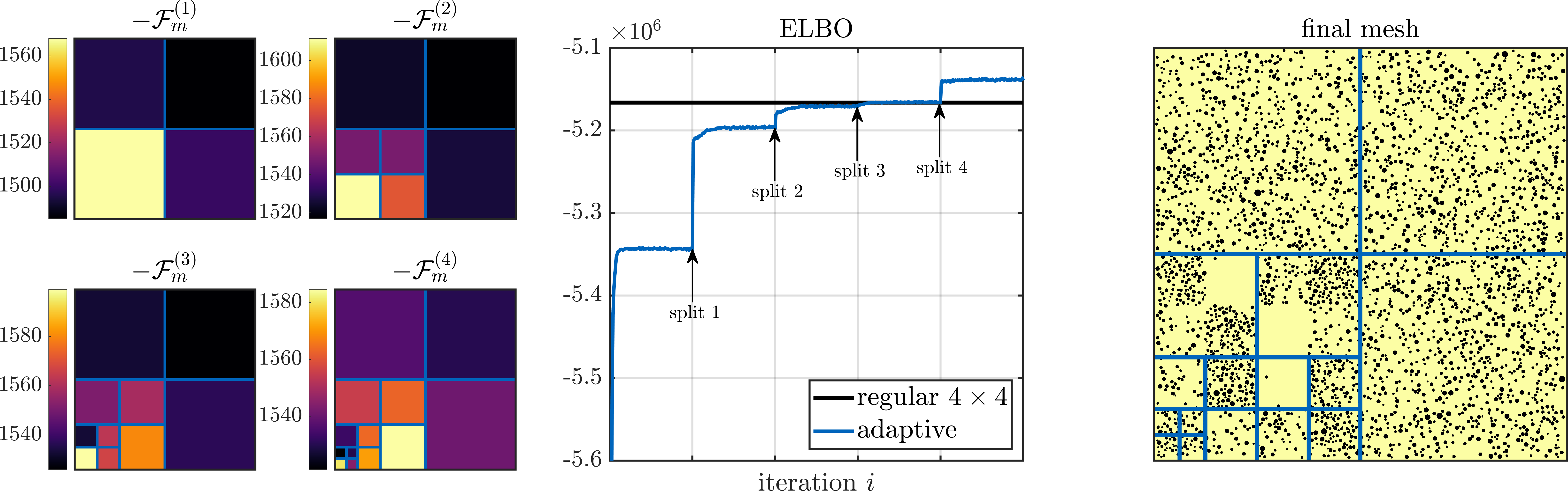
Figure 17 depicts the process of 4 successive splits each of which corresponds to dividing the selected cell into four equal-sized squares. Hence the number of cells/subregions and therefore the dimension of the associated will become and after each of the aforementioned splits. The left part of Figure 17 shows the cell scores computed as in Equation (45) right before each split. The cell that is subsequently subdivided is the one with the lowest . As expected, the splits are concentrated in the lower-left quadrant and the right part of the Figure shows the corresponding discretization of the permeability field after the 4 splits. The tendency to refine close to the origin (lower left corner) and along the lower boundary may be explained by the fact that the microstructures are constructed such that solid phase exclusions have a minimum distance of to the domain boundary, i.e. there always exists a narrow path along the boundaries where fluid can flow. As boundary conditions imply flux from left to right, it is beneficial to refine close to the lower domain boundary. The lower left corner is further distinguished by the fact that the pressure boundary condition is implied here.
More importantly, the middle part of 17 shows the evolution of the ELBO over training iterations (blue line). The jumps that are observed after each split are a result of the improvement in the model which is to be expected due to the increased dimension . We also compare the ELBO score after 4 splits (where ) with a regular discretization of the Darcy permeability into squares in which as well, i.e. the dimension of the information bottleneck variables is the same. We note that the adaptive refinement proposed leads to an improved final model.
4 Conclusions
We have presented a physics-informed, fully Bayesian surrogate model to predict response fields of stochastic partial differential equations with high-dimensional stochastic input as those arising in random heterogeneous media. Employing an encoder-decoder architecture with a coarse-grained model (CGM) based on simplified physics as a stencil at its core, it is possible to provide tight and accurate probabilistic predictions even when the training data i.e. fine-grained model simulations, is scarce (i.e. of the order of ) and the stochastic input dimension is large (i.e. or larger). The encoding or coarse-graining step is capable of extracting the salient features of the input random field which are most predictive of the fine-scale PDE-response, thereby drastically reducing the stochastic input dimension in an optimal way. This low-dimensional, latent representation then serves as the input to the CGM, the output of which is basal for the probabilistic reconstruction of the fine scale output. Predictive uncertainty due to limited training data as well as due to the information loss unavoidably taking place during the coarse-graining step is accurately quantified by the fully probabilistic nature of the model. All parts of the model were trained simultaneously in a fully Bayesian way using Stochastic Variational Inference, without the need of any parameters to be specified by the analyst.
On the basis of the Stokes/Darcy similarity for flow through random porous media, we provided numerical evidence of the predictive capabilities under the aforementioned setting. Another important advantage of the proposed formulation is its ability to perform comparably well under extrapolative conditions. In the context of the models explored, we demonstrated this by carrying out predictions on data under a considerably different (or even randomized) boundary conditions than those used for training. Furthermore, we demonstrated one of the many possible application of the proposed model for Uncertainty Propagation problems where not only accurate estimates of output statistics but the confidence in these predictions is quantified. Finally, we outlined a method for automatically and adaptively refining the model and demonstrated its benefits in the context of the problems explored.
Applications of the proposed model can be found in any multi-query setting with expensive forward model evaluations, as is often the case in design-, optimization- or inverse problems. Several model extensions can be contemplated. For coarse-graining of the high-dimensional stochastic inputs, a deep learning framework could be adopted, potentially benefiting from recent advances in computer vision with e.g. convolutional neural networks (CNNs) or deep Gaussian process models. We emphasize however that significant regularization would be needed to make those work in the Small Data setting considered. Furthermore, one might think of a model that not only passes information through the CGM, but also entails ‘bypassing’ components, thereby effectively expanding the information bottleneck and allowing for more detailed reconstruction of fine scale output variability.
Appendix A Optimizing the variational distributions
To maximize the ELBO functional in equation (25) w.r.t. the variational distributions under the normalization constraint , we maximize the functional
| (63) |
where is a subset of the model parameters and are Lagrangean multipliers. The first order variation w.r.t. is
| (64) |
where . As for arbitrary ,
| (65) |
or
| (66) |
where denotes the expected value w.r.t. . The normalization constraints are recaptured by and determine the constant in Equation (66). Thus, it is found that
| (67) |
A.1 Black-box variational inference for
We note that minimization of the KL divergence as given in equation (35) is equivalent to
| (68) |
where is the Shannon entropy of . Expected values of terms in (68) depending on the CGM are analytically intractable and gradients w.r.t. are therefore only accesible by noisy Monte Carlo estimates. To reduce the variance in those estimates, we apply the reparametrization trick Kingma and Welling 2013
| (69) |
and express Equation (68) as
| (70) |
where ‘’ denotes element-wise multiplication and we used the fact that
. Derivatives w.r.t. , can be computed using the chain rule as
| (71) | ||||
| (72) | ||||
| (73) |
where and . To solve the optimization problem in (70), the above gradients are passed to the adaptive moment estimation optimizer (ADAM) using the default optimization parameters suggested in Kingma and Ba 2014.
Appendix B Feature functions
Feature functions
| Index | Function | Comment |
| 1 | constant | |
| 2 | pore fraction in | pore fraction evaluated on full domain |
| 3 | pore fraction in | |
| 4–7 | (pore fraction)0.5…0.5…2.5 in | |
| 8 | (pore fraction) | |
| 9 | SCA in | self-cons. approx. Torquato 2001, sec. 18.1.2, inf. contrast limit |
| 10 | Maxwell-Approximation in | inf. contrast limit, see Torquato 2001, sec. 18.2.1 |
| 11 | Maxwell-Approximation | |
| 12–17 | chord length density in , | see Torquato 2001 sec. 6.2.4 |
| 18 | interface area in | |
| 19 | interface area in | |
| 20–27 | interface area in | |
| 28–31 | (interface area)1/3,1/4,1/5,2 in | |
| 32 | mean distance edge in | measured from excl. edge to edge |
| 33 | mean distance edge in | measured from excl. edge to edge |
| 34 | mean distance edge in | measured from excl. edge to edge |
| 35 | mean distance edge in | measured from excl. edge to edge |
| 36 | mean distance center in | measured from excl. center to center |
| 37 | min. distance center in | measured from excl. center to center |
| 38 | min. distance center in | measured from excl. center to center |
| 39 | min. distance center in | measured from excl. center to center |
| 40–43 | lineal path in for | see Torquato 2001, sec. 2.4 |
| 44–47 | lineal path in for | |
| 48 | void nearest-neighbor pdf, , in | see Torquato 2001, sec. 2.8 |
| 49 | void nearest-neighbor pdf, , in | see Torquato 2001. sec. 2.8 |
| 50 | pore size density, , in | see Torquato 2001, sec. 2.6 |
| 51 | pore size density, , in | see Torquato 2001, sec. 2.6 |
| 52 | mean chord length in | see Torquato 2001, sec. 2.5 |
| 53 | mean chord length in | see Torquato 2001, sec. 2.5 |
| 54 | mean chord length in | see Torquato 2001, sec. 2.5 |
| 55 | (mean chord length)0.5 in | see Torquato 2001, sec. 2.5 |
| 56–58 | in | expected exclusion radii moments |
| 59–61 | in | expected exclusion radii moments |
| 62 | pore fraction in | |
| 63 | pore fraction in | |
| 64 | pore fraction in | |
| 65–68 | (pore fraction)0.5,1.5,2,2.5 in | |
| 69 | self-consistent approximation (inf. contrast) in | |
| 70 | Maxwell Approximation in | |
| 71 | Maxwell Approximation in | |
| 72–78 | chord length dens. in , | |
| 79 | interface area in | |
| 80–88 | interface area in | |
| 89–93 | interface area in | |
| 94 | mean distance edge in | measured from excl. edge to edge |
| 95 | mean distance edge in | measured from excl. edge to edge |
| 96 | max distance edge in | measured from excl. edge to edge |
| 97 | max distance edge in | measured from excl. edge to edge |
| 98 | std distance edge in | measured from excl. edge to edge |
| 99 | std distance edge in | measured from excl. edge to edge |
| 100–104 | square well potential, width = in | |
| 105 | mean distance in | measured from excl. edge to edge |
| 106 | mean distance in | measured from excl. edge to edge |
| 107 | mean distance center in | measured from excl. center to center |
| 108 | min. distance center in | measured from excl. center to center |
| 109 | min. distance center in | measured from excl. center to center |
| 110 | min. distance center in | measured from excl. center to center |
| 111–114 | lineal path in for | |
| 115–118 | lineal path in for | |
| 119 | void nearest-neighbor pdf, , in | see Torquato 2001, sec. 2.8 |
| 120 | void nearest-neighbor pdf, , in | see Torquato 2001. sec. 2.8 |
| 121 | pore size density, , in | see Torquato 2001, sec. 2.6 |
| 122 | pore size density, , in | see Torquato 2001, sec. 2.6 |
| 123 | mean chord length in | see Torquato 2001, sec. 2.5 |
| 124 | mean chord length in | see Torquato 2001, sec. 2.5 |
| 125 | mean chord length in | see Torquato 2001, sec. 2.5 |
| 126 | (mean chord length)0.5 in | see Torquato 2001, sec. 2.5 |
| 127–129 | in | expected exclusion radii moments |
| 130–132 | in | expected exclusion radii moments |
| 133 | length scale of exp. approx. to lin. path in | |
| 134 | mean of euclidean dist. transform in | see Soille 1999 |
| 135 | variance of euclidean dist. transform in | see Soille 1999 |
| 136 | max. of euclidean dist. transform in | see Soille 1999 |
| 137 | mean of chessboard dist. transform in | see Soille 1999 |
| 138 | variance of chessboard dist. transform in | see Soille 1999 |
| 139 | max. of chessboard dist. transform in | see Soille 1999 |
| 140 | mean of cityblock dist. transform in | see Soille 1999 |
| 141 | variance of cityblock dist. transform in | see Soille 1999 |
| 142 | max. of cityblock dist. transform in | see Soille 1999 |
| 143–145 | Gauss lin. filt. pixels in | see Grigo and Koutsourelakis 2019 |
| 146 | Ising energy in | |
| 147 | shortest connected path, -dir., Euclidean, in | see Soille 1999 |
| 148 | shortest connected path, -dir., Euclidean, in | see Soille 1999 |
| 149 | shortest connected path, -dir., cityblock, in | see Soille 1999 |
| 150 | shortest connected path, -dir., cityblock, in | see Soille 1999 |
Appendix C Proper orthogonal decomposition of output data
In section 3.2, it is mentioned that we observe very fast decay of POD eigenmodes for data with large variance in the pore space fraction , which translates to high as explained in section 3.1.1. We therefore plot the explained PCA variance, i.e. the cumulative sum of the largest variances of a PCA analysis performed on 2048 sample vectors for the data used in sections 3.2 and 3.3 in figure 18. We note that this fast decay in POD eigenmodes observed in section 3.2 does not affect the effective input dimensionality of . To show that, we discretize the 2048 microstructures from the distributions defined in sections 3.2, 3.3 to bitmap image vectors of dimensions and again plot the explained variance from the first components in the second row of figure 18. We observe that our claim of high-dimensional inputs is verified, as the explained variance is only slowly increasing with the number of POD components.
Appendix D Evidence Lower BOund (ELBO)
Using the expected values found in equations (28)–(32), omitting constants and canceling terms, we find
| (74) |
as the most compact form of the evidence lower bound (ELBO) . We note that with the exception of the first term, the remaining ones are automatically separated into additive contributions from each cell or equivalently each . Hence, in order to arrive at the cell-scoring function given in Equation (45), we pick out the terms in equation (74) which explicitly carry a cell index . These are
In the numerical experiments, we tie the precision parameters across different cells together i.e. which allows sharing of information in terms of the microstructural features. As a result and the corresponding contribution from each cell becomes:
| (75) |
References
- Ghahramani (2015) Z. Ghahramani, Probabilistic machine learning and artificial intelligence, Nature 521 (2015) 452–459.
- LeCun et al. (2015) Y. LeCun, Y. Bengio, G. Hinton, Deep learning, Nature 521 (2015) 436–444.
- Goodfellow et al. (2016) I. Goodfellow, Y. Bengio, A. Courville, Deep Learning, MIT Press, 2016. http://www.deeplearningbook.org.
- Koutsourelakis et al. (2016) P. S. Koutsourelakis, N. Zabaras, M. Girolami, Special Issue: Big data and predictive computational modeling, Journal of Computational Physics 321 (2016) 1252–1254.
- Wiener (1938) N. Wiener, The Homogeneous Chaos, American Journal of Mathematics 60 (1938) 897–936.
- Ghanem and Spanos (1991) R. G. Ghanem, P. D. Spanos, Stochastic Finite Elements: A Spectral Approach, Springer, New York, 1991. URL: http://cds.cern.ch/record/1622736.
- Xiu and Karniadakis (2002) D. Xiu, G. Karniadakis, The Wiener–Askey Polynomial Chaos for Stochastic Differential Equations, SIAM Journal on Scientific Computing 24 (2002) 619–644.
- Xiu and Hesthaven (2005) D. Xiu, J. Hesthaven, High-Order Collocation Methods for Differential Equations with Random Inputs, SIAM Journal on Scientific Computing 27 (2005) 1118–1139.
- Ma and Zabaras (2009) X. Ma, N. Zabaras, An adaptive hierarchical sparse grid collocation algorithm for the solution of stochastic differential equations, Journal of Computational Physics 228 (2009) 3084 – 3113.
- Lin and Tartakovsky (2009) G. Lin, A. Tartakovsky, An efficient, high-order probabilistic collocation method on sparse grids for three-dimensional flow and solute transport in randomly heterogeneous porous media, Advances in Water Resources 32 (2009) 712 – 722. Dispersion in Porous Media.
- Lin et al. (2010) G. Lin, A. Tartakovsky, D. Tartakovsky, Uncertainty quantification via random domain decomposition and probabilistic collocation on sparse grids, Journal of Computational Physics 229 (2010) 6995 – 7012.
- Tipireddy et al. (2017) R. Tipireddy, P. Stinis, A. Tartakovsky, Basis adaptation and domain decomposition for steady-state partial differential equations with random coefficients, Journal of Computational Physics 351 (2017) 203 – 215.
- Tipireddy et al. (2018) R. Tipireddy, P. Stinis, A. Tartakovsky, Stochastic Basis Adaptation and Spatial Domain Decomposition for Partial Differential Equations with Random Coefficients, SIAM/ASA Journal on Uncertainty Quantification 6 (2018) 273–301.
- Torquato and Lu (1993) S. Torquato, B. Lu, Chord-length distribution function for two-phase random media, Phys. Rev. E 47 (1993) 2950–2953.
- Bilionis et al. (2013) I. Bilionis, N. Zabaras, B. A. Konomi, G. Lin, Multi-output separable Gaussian process: Towards an efficient, fully Bayesian paradigm for uncertainty quantification, Journal of Computational Physics 241 (2013) 212 – 239.
- Atkinson and Zabaras (2019) S. Atkinson, N. Zabaras, Structured Bayesian Gaussian process latent variable model: Applications to data-driven dimensionality reduction and high-dimensional inversion, Journal of Computational Physics (2019).
- Mo et al. (2018) S. Mo, Y. Zhu, N. Zabaras, X. Shi, J. Wu, Deep Convolutional Encoder-Decoder Networks for Uncertainty Quantification of Dynamic Multiphase Flow in Heterogeneous Media, Water Resources Research 0 (2018).
- Chauvière et al. (2006) C. Chauvière, J. Hesthaven, L. Lurati, Computational Modeling of Uncertainty in Time-Domain Electromagnetics, SIAM Journal on Scientific Computing 28 (2006) 751–775.
- O’Hagan and Kennedy (2000) A. O’Hagan, M. Kennedy, Predicting the output from a complex computer code when fast approximations are available, Biometrika 87 (2000) 1–13.
- Koutsourelakis (2009) P.-S. Koutsourelakis, Accurate Uncertainty Quantification Using Inaccurate Computational Models, SIAM Journal on Scientific Computing 31 (2009) 3274–3300.
- Perdikaris et al. (2017) P. Perdikaris, M. Raissi, A. Damianou, N. D. Lawrence, G. E. Karniadakis, Nonlinear information fusion algorithms for data-efficient multi-fidelity modelling, Proceedings of the Royal Society A: Mathematical, Physical and Engineering Science 473 (2017) 20160751.
- Hesthaven et al. (2016) J. Hesthaven, G. Rozza, B. Stamm, Certified Reduced Basis Methods for Parametrized Partial Differential Equations, Springer Briefs in Mathematics, Springer International Publishing, 2016. URL: //www.springer.com/de/book/9783319224695.
- Quarteroni et al. (2016) A. Quarteroni, A. Manzoni, F. Negri, Reduced Basis Methods for Partial Differential Equations. An Introduction, La Matematica per il 3+2. 92, Springer International Publishing, 2016. URL: http://infoscience.epfl.ch/record/218966. doi:10.1007/978-3-319-15431-2.
- Rowley et al. (2004) C. W. Rowley, T. Colonius, R. M. Murray, Model reduction for compressible flows using POD and Galerkin projection, Physica D: Nonlinear Phenomena 189 (2004) 115 – 129.
- Cui et al. (2015) T. Cui, Y. Marzouk, K. Willcox, Data-driven model reduction for the bayesian solution of inverse problems, International Journal for Numerical Methods in Engineering 102 (2015) 966–990.
- Afkham and Hesthaven (2017) B. Afkham, J. Hesthaven, Structure Preserving Model Reduction of Parametric Hamiltonian Systems, SIAM Journal on Scientific Computing 39 (2017) A2616–A2644.
- Yu and Hesthaven (2018) J. Yu, J. Hesthaven, Flowfield Reconstruction Method Using Artificial Neural Network, AIAA Journal (2018) 1–17.
- Guo and Hesthaven (2018) M. Guo, J. Hesthaven, Reduced order modeling for nonlinear structural analysis using gaussian process regression, Computer Methods in Applied Mechanics and Engineering 341 (2018) 807 – 826.
- Hesthaven and Ubbiali (2018) J. Hesthaven, S. Ubbiali, Non-intrusive reduced order modeling of nonlinear problems using neural networks, Journal of Computational Physics 363 (2018) 55 – 78.
- Rasmussen and Williams (2006) C. Rasmussen, C. Williams, Gaussian Processes for Machine Learning, Adaptive Computation and Machine Learning, MIT Press, Cambridge, MA, USA, 2006.
- Bilionis and Zabaras (2017) I. Bilionis, N. Zabaras, Bayesian Uncertainty Propagation Using Gaussian Processes, Springer International Publishing, Cham, 2017, pp. 555–599. URL: https://doi.org/10.1007/978-3-319-12385-1_16. doi:10.1007/978-3-319-12385-1_16.
- Raissi et al. (2017) M. Raissi, P. Perdikaris, G. E. Karniadakis, Inferring solutions of differential equations using noisy multi-fidelity data, Journal of Computational Physics 335 (2017) 736 – 746.
- Perdikaris et al. (2015) P. Perdikaris, D. Venturi, J. O. Royset, G. E. Karniadakis, Multi-fidelity modelling via recursive co-kriging and Gaussian–Markov random fields, Proceedings of the Royal Society A: Mathematical, Physical and Engineering Sciences 471 (2015) 20150018.
- Raissi and Karniadakis (2018) M. Raissi, G. E. Karniadakis, Hidden physics models: Machine learning of nonlinear partial differential equations, Journal of Computational Physics 357 (2018) 125 – 141.
- Yang et al. (2018) X. Yang, G. Tartakovsky, A. Tartakovsky, Physics-Informed Kriging: A Physics-Informed Gaussian Process Regression Method for Data-Model Convergence, arxiv e-print (2018).
- Lee et al. (2018) S. Lee, F. Dietrich, G. Karniadakis, I. Kevrekidis, Linking Gaussian Process regression with data-driven manifold embeddings for nonlinear data fusion, arxiv e-print (2018).
- Tipireddy and Tartakovsky (2018) R. Tipireddy, A. Tartakovsky, Physics-informed Machine Learning Method for Forecasting and Uncertainty Quantification of Partially Observed and Unobserved States in Power Grids, arxiv e-print (2018).
- Tripathy and Bilionis (2018) R. Tripathy, I. Bilionis, Deep UQ: Learning deep neural network surrogate models for high dimensional uncertainty quantification, arXiv:1802.00850 [physics, stat] (2018).
- Zhu and Zabaras (2018) Y. Zhu, N. Zabaras, Bayesian deep convolutional encoder–decoder networks for surrogate modeling and uncertainty quantification, Journal of Computational Physics 366 (2018) 415 – 447.
- Yang and Perdikaris (2019) Y. Yang, P. Perdikaris, Conditional deep surrogate models for stochastic, high-dimensional, and multi-fidelity systems, arxiv e-print (2019).
- Raissi et al. (2017) M. Raissi, P. Perdikaris, G. Karniadakis, Physics Informed Deep Learning (Part I): Data-driven Solutions of Nonlinear Partial Differential Equations, arxiv e-print (2017).
- Raissi et al. (2019) M. Raissi, P. Perdikaris, G. Karniadakis, Physics-informed neural networks: A deep learning framework for solving forward and inverse problems involving nonlinear partial differential equations, Journal of Computational Physics 378 (2019) 686 – 707.
- Tartakovsky et al. (2018) A. Tartakovsky, C. O. Marrero, P. Perdikaris, G. Tartakovsky, D. Barajas-Solano, Learning Parameters and Constitutive Relationships with Physics Informed Deep Neural Networks, arxiv e-print (2018).
- Raissi et al. (2017) M. Raissi, P. Perdikaris, G. E. Karniadakis, Physics informed deep learning (part ii): data-driven discovery of nonlinear partial differential equations, arXiv preprint arXiv:1711.10566 (2017).
- Zhu et al. (2019) Y. Zhu, N. Zabaras, P.-S. Koutsourelakis, P. Perdikaris, Physics-Constrained Deep Learning for High-dimensional Surrogate Modeling and Uncertainty Quantification without Labeled Data, Journal of Computational Physics (2019). Submitted for publication.
- Schöberl et al. (2017) M. Schöberl, N. Zabaras, P.-S. Koutsourelakis, Predictive coarse-graining, Journal of Computational Physics 333 (2017) 49–77.
- Ma and Zabaras (2011) X. Ma, N. Zabaras, Kernel principal component analysis for stochastic input model generation, Journal of Computational Physics 230 (2011) 7311 – 7331.
- Xing et al. (2016) W. W. Xing, V. Triantafyllidis, A. A. Shah, P. B. Nair, N. Zabaras, Manifold learning for the emulation of spatial fields from computational models, Journal of Computational Physics 326 (2016) 666–690.
- Paisley et al. (2012) J. Paisley, D. Blei, M. I. Jordan, Variational Bayesian inference with stochastic search, 29th International Conference on Machine Learning (ICML) (2012).
- Hoffman et al. (2013) M. D. Hoffman, D. M. Blei, C. Wang, J. Paisley, Stochastic Variational Inference, J. Mach. Learn. Res. 14 (2013) 1303–1347.
- Kingma and Ba (2014) D. P. Kingma, J. Ba, Adam: A Method for Stochastic Optimization, CoRR abs/1412.6980 (2014).
- Bishop and Tipping (2000) C. M. Bishop, M. E. Tipping, Variational Relevance Vector Machines, in: Proceedings of the Sixteenth Conference on Uncertainty in Artificial Intelligence, UAI’00, Morgan Kaufmann Publishers Inc., San Francisco, CA, USA, 2000, pp. 46–53. URL: http://dl.acm.org/citation.cfm?id=2073946.2073953.
- Tishby et al. (1999) N. Tishby, F. C. Pereira, W. Bialek, The Information Bottleneck Method, in: Proc. of the 37-th Annual Allerton Conference on Communication, Control and Computing, 1999, pp. 368–377. URL: /brokenurl#citeseer.nj.nec.com/tishby99information.html.
- Grigo and Koutsourelakis (2017) C. Grigo, P.-S. Koutsourelakis, Probabilistic reduced-order modeling for stochastic partial differential equations, in: 2nd International Conference on Uncertainty Quantification in Computational Sciences and Engineering, Eccomas Thematic Conferences, 2017, pp. 111–129. URL: https://www.eccomasproceedia.org/conferences/thematic-conferences/uncecomp-2017/5356.
- Grigo and Koutsourelakis (2019) C. Grigo, P. Koutsourelakis, Bayesian model and dimension reduction for uncertainty propagation: Applications in random media, SIAM/ASA Journal on Uncertainty Quantification 7 (2019) 292–323.
- Logg et al. (2012) A. Logg, K.-A. Mardal, G. N. Wells, et al., Automated Solution of Differential Equations by the Finite Element Method, Springer, 2012. doi:10.1007/978-3-642-23099-8.
- Sanchez-Palencia (1980) E. Sanchez-Palencia, Non-Homogeneous Media and Vibration Theory, Lecture Notes in Physics 127 (1980).
- Tartar (1980) L. Tartar, Incompressible fluid flow in a porous medium-convergence of the homogenization process, Appendix of Sanchez-Palencia 1980 (1980).
- Allaire (1989) G. Allaire, Homogenization of the stokes flow in a connected porous medium, Asymptotic Analysis 2 (1989) 203–222.
- Allaire (1992) G. Allaire, Homogenization of the unsteady Stokes equations in porous media, volume 267 of Pitman Research Notes in Mathematics Series, Longman Higher Education, New York, 1992, pp. 109–123. URL: http://www.cmap.polytechnique.fr/~allaire/unsteady-stokes.pdf.
- Whitaker (1986) S. Whitaker, ”Flow in porous media I: A theoretical derivation of Darcy’s law”, Transport in Porous Media 1 (1986) 3–25.
- Sandström et al. (2013) C. Sandström, F. Larsson, K. Runesson, H. Johansson, A two-scale finite element formulation of Stokes flow in porous media, Computer Methods in Applied Mechanics and Engineering 261-262 (2013) 96 – 104.
- Marchenko and Khruslov (2006) V. Marchenko, E. Khruslov, Homogenization of Partial Differential Equations, Birkhäuser Boston, Boston, MA, 2006. URL: https://doi.org/10.1007/978-0-8176-4468-0_1. doi:10.1007/978-0-8176-4468-0_1.
- Tartar (2010) L. Tartar, The General Theory of Homogenization: A Personalized Introduction, Springer Berlin Heidelberg, Berlin, Heidelberg, 2010. URL: https://doi.org/10.1007/978-3-642-05195-1_1. doi:10.1007/978-3-642-05195-1_1.
- Fukushima (1980) K. Fukushima, Neocognitron - a Self-Organizing Neural Network Model for a Mechanism of Pattern-Recognition Unaffected by Shift in Position, Biological Cybernetics 36 (1980) 193–202.
- Lecun et al. (1998) Y. Lecun, L. Bottou, Y. Bengio, P. Haffner, Gradient-based learning applied to document recognition, Proceedings of the Ieee 86 (1998) 2278–2324.
- Krizhevsky et al. (2012) A. Krizhevsky, I. Sutskever, G. E. Hinton, Imagenet classification with deep convolutional neural networks, in: F. Pereira, C. J. C. Burges, L. Bottou, K. Q. Weinberger (Eds.), Advances in Neural Information Processing Systems 25, Curran Associates, Inc., 2012, pp. 1097–1105. URL: http://papers.nips.cc/paper/4824-imagenet-classification-with-deep-convolutional-neural-networks.pdf.
- Torquato (2001) S. Torquato, Random Heterogeneous Materials, Springer, 2001.
- Lu and Torquato (1992) B. Lu, S. Torquato, Lineal-path function for random heterogeneous materials, Phys. Rev. A 45 (1992) 922–929.
- Lowell et al. (2006) S. Lowell, J. E. Shields, M. A. Thomas, M. Thommes, Characterization of Porous Solids and Powders: Surface Area, Pore Size and Density, volume 1, Springer, 2006.
- Sutera and Skalak (1993) S. P. Sutera, R. Skalak, The History of Poiseuille’s Law, Annual Review of Fluid Mechanics 25 (1993) 1–20.
- Kozeny (1927) J. Kozeny, Ueber Kapillare Leitung der Wasser in Boden, Royal Academy of Science, Vienna, Proc. Class I 136 (1927) 271–306.
- Carman (1937) P. C. Carman, Fluid Flow through Granular Beds, Trans. Inst. Chem. Eng. 15 (1937) 150–166.
- Archie (1947) G. E. Archie, Electrical resistivity an aid in core-analysis interpretation, AAPG Bulletin 31 (1947) 350.
- Soille (1999) P. Soille, Morphological Image Analysis: Principles and Applications, Springer-Verlag Berlin Heidelberg, Berlin, DE, 1999, pp. 89–125.
- Doersch (2016) C. Doersch, Tutorial on Variational Autoencoders, 2016.
- Bruggeman (1935) D. A. G. Bruggeman, Berechnung verschiedener physikalischer konstanten von heterogenen substanzen. i. dielektrizitätskonstanten und leitfähigkeiten der mischkörper aus isotropen substanzen, Annalen der Physik 416 (1935) 636–664.
- Landauer (1978) R. Landauer, Electrical conductivity in inhomogeneous media, AIP Conference Proceedings 40 (1978) 2–45.
- Lawrence (2005) N. D. Lawrence, Probabilistic Non-linear Principal Component Analysis with Gaussian Process Latent Variable Models, Journal of Machine Learning Research 6 (2005) 1783–1816.
- Titsias and Lawrence (2010) M. K. Titsias, N. D. Lawrence, Bayesian Gaussian Process Latent Variable Model, in: Y. W. Teh, D. M. Titterington (Eds.), Proceedings of the Thirteenth International Conference on Artificial Intelligence and Statistics, AISTATS 2010, Chia Laguna Resort, Sardinia, Italy, May 13-15, 2010, volume 9 of JMLR Proceedings, JMLR.org, 2010, pp. 844–851. URL: http://www.jmlr.org/proceedings/papers/v9/titsias10a.html.
- Damianou et al. (2015) A. C. Damianou, M. K. Titsias, N. D. Lawrence, Variational Inference for Latent Variables and Uncertain Inputs in Gaussian Processes, Journal of Machine Learning Research (JMLR) 2 (2015).
- Faul (2003) A. C. Faul, Analysis of sparse Bayesian learning, Advances in Neural Information Processing Systems (NIPS) 14 (2003) 383–389.
- Tipping (2001) M. E. Tipping, Sparse Bayesian learning and the relevance vector machine, J. Machine Learning Research (2001).
- Gelman et al. (2003) A. Gelman, J. Carlin, H. Stern, D. Rubin, Bayesian Data Analysis, 2nd ed., Chapman & Hall/CRC, 2003.
- Blei et al. (2017) D. M. Blei, A. Kucukelbir, J. D. McAuliffe, Variational inference: A review for statisticians, Journal of the American Statistical Association 112 (2017) 859–877.
- Beal and Ghahramani (2003) M. J. Beal, Z. Ghahramani, The Variational Bayesian EM Algorithm for Incomplete Data: with Application to Scoring Graphical Model Structures, Bayesian Statistics 7 (2003).
- Ranganath et al. (2014) R. Ranganath, S. Gerrish, D. Blei, Black Box Variational Inference, in: S. Kaski, J. Corander (Eds.), Proceedings of the Seventeenth International Conference on Artificial Intelligence and Statistics, volume 33 of Proceedings of Machine Learning Research, PMLR, Reykjavik, Iceland, 2014, pp. 814–822. URL: http://proceedings.mlr.press/v33/ranganath14.html.
- Heinkenschloss (2008) M. Heinkenschloss, Numerical solution of implicitly constrained optimization problems, Rice University Department of Computational and applied Mathematics 05 (2008) 1–25.
- Constantine et al. (2014) P. Constantine, E. Dow, Q. Wang, Active Subspace Methods in Theory and Practice: Applications to Kriging Surfaces, SIAM Journal on Scientific Computing 36 (2014) A1500–A1524.
- Kingma and Welling (2013) D. P. Kingma, M. Welling, Auto-Encoding Variational Bayes, CoRR abs/1312.6114 (2013).
- Zhang (2017) D. Zhang, A Coefficient of Determination for Generalized Linear Models, The American Statistician 71 (2017) 310–316.
- Murray and Ghahramani (2005) I. Murray, Z. Ghahramani, A note on the evidence and Bayesian Occam’s razor, Technical Report, Gatsby Unit Technical Report GCNU-TR 2005-003, 2005.
- Rasmussen and Ghahramani (2001) C. Rasmussen, Z. Ghahramani, Occam’s Razor, in: Neural Information Processing Systems 13, 2001, pp. 294–300.
- Ghahramani and Beal (2000) Z. Ghahramani, M. J. Beal, Variational inference for Bayesian mixtures of factor analysers, NIPS 12 (2000).