Field theory and structure-preserving geometric particle-in-cell algorithm for drift wave instability and turbulence
Abstract
A field theory and the associated structure-preserving geometric Particle-In-Cell (PIC) algorithm are developed to study low frequency electrostatic perturbations with fully kinetic ions and adiabatic electrons in magnetized plasmas. The algorithm is constructed by geometrically discretizing the field theory using discrete exterior calculus, high-order Whitney interpolation forms, and non-canonical Hamiltonian splitting method. The discretization preserves the non-canonical symplectic structure of the particle-field system, as well as the electromagnetic gauge symmetry. As a result, the algorithm is charge-conserving and possesses long-term conservation properties. Because drift wave turbulence and anomalous transport intrinsically involve multi time-scales, simulation studies using fully kinetic particle demand algorithms with long-term accuracy and fidelity. The structure-preserving geometric PIC algorithm developed adequately servers this purpose. The algorithm has been implemented in the SymPIC code, tested and benchmarked using the examples of ion Bernstein waves and drift waves. We apply the algorithm to study the Ion Temperature Gradient (ITG) instability and turbulence in a 2D slab geometry. Simulation results show that at the early stage of the turbulence, the energy diffusion is between the Bohm scaling and gyro-Bohm scaling. At later time, the observed diffusion is closer to the gyro-Bohm scaling, and density blobs generated by the rupture of unstable modes are the prominent structures of the fully developed ITG turbulence.
Keywords:
Structure-preserving geometric algorithm, particle-in-cell, drift wave instability, ion temperature gradient turbulencepacs
52.65.Rr, 52.25.Dg1 Introduction
Drift wave turbulence and associated anomalous transport Krall and Rosenbluth 1965; Coppi 1967; Tang 1978; Horton 1999 are important physical processes in magnetic fusion devices. They have been intensively studied using the Particle-In-Cell (PIC) methods Dawson 1983; Hockney and Eastwood 1988; Birdsall and Langdon 1991, which numerically solve the Vlasov-Maxwell or Vlasov-Poisson equations. The dynamics of charged particles in a magnetic field described by the Vlasov equation contains multiple timescales, e.g., the cyclotron frequencies of electrons and ions, plasma frequency, and the drift wave frequency. When simulating low frequency phenomena directly using the PIC method, the time-step must be chosen small enough to resolve the high frequency dynamics of charged particles. Thus, the total number of time-steps required is large, often exceeding computer resource available. The low frequency drift wave instability is such a case, where the ratio between wave frequency and the electron gyro-frequency is in the order of . To overcome this difficulty, simplified models which eliminate some of the high-frequency processes while properly describing the slow ion dynamics are developed. A commonly adopted such kinetic model is based on adiabatic electron assumption and quasi-neutrality condition. In this model, for plasmas with one ion species, the ion density , electrons density , and the electrostatic potential are linked as
| (1) |
where and are the charges of ions and electrons, and is the electron temperature. The ion dynamics is governed by Newton’s equation with the Lorentz force,
| (2) |
where is the background magnetic field, is the electric field, and is the background electric field.
To further decrease computational complexity, gyrokinetic particle simulation methods have been developed and applied to study low frequency instabilities and turbulent transport Lee 1983; Dimits and Lee 1993; Parker and Lee 1993; Parker et al. 1993; Hu and Krommes 1994; Dimits et al. 1996; Lin et al. 1998; Parker et al. 1999. In spite of the success of gyrokinetic simulations, it was pointed out recently that the basic ordering of the gyrokinetic theory Frieman et al. 1966; Catto 1978; Frieman and Chen 1982; Dubin et al. 1983; Hahm 1988; Brizard 1989; Qin et al. 1998; Qin et al. 2000; Qin and Tang 2004; Qin 2005; Qin et al. 2007; Burby 2015; Burby et al. 2015 is not always valid in certain parameter regimes for modern magnetic fusion devices, especially for the H-mode pedestal physics Wan and Parker 2012; Wan et al. 2013 and when density perturbations are large Deng and Waltz 2015. Moreover, due to the requirement of accuracy and numerical stability, the time-step in gyrokinetic simulations are often restricted to the same order of ion gyro-period Chen et al. 2008; Chowdhury et al. 2016 already. In these situations, the gyrokinetic method has no significant computational advantage over fully kinetic methods. Recently, a fully kinetic ion scheme was developed Miecnikowski et al. 2018; Sturdevant et al. 2017; Hu et al. 2018. However, even though adiabatic electron model removes the fast electron dynamics from the system, drift wave instabilities and turbulence still evolve in a slow timescale, about one thousandth of ion gyro-period. Simulating these low frequency physics using fully kinetic ions requires a large number of time-steps, and the long-term conservative properties of the numerical schemes become crucial. Conventional PIC methods are based on direct discretization of differential equations, for which numerical errors in general accumulate coherently during the iterations, and long-term simulation results are not reliable.
In the present study, we use a very different approach to construct an explicit high-order structure-preserving geometric PIC algorithm for simulating low frequency drift wave instabilities and turbulence in magnetized plasmas. First, a field theory for low frequency electrostatic dynamics is established with fully kinetic ions and adiabatic electrons. Then the field theory is geometrically discretized using Discrete Exterior Calculus (DEC) Hirani 2003; Desbrun et al., Whitney interpolating forms Whitney 1957; Squire et al. 2012a; Squire et al. 2012b; Xiao et al. 2015a, and the powerful Hamiltonian splitting method for Vlasov-Maxwell systems Xiao et al. 2015a; He et al. 2015a; He et al. 2017. The resulting structure-preserving geometric PIC algorithm is able to preserve the non-canonical symplectic structure associated with the particle-field system, and numerical results show that the simulation error on the energy of the system is bounded by a small number for all time-steps. In addition, the algorithm is gauge independent and thus exactly complies with the discrete local charge conservation law. The knowledge of magnetic potentials is not needed, which is convenient in practical. Furthermore, the algorithm is locally explicit such that it is more efficient on parallel clusters compared with implicit schemes.
In the last ten years, structure-preserving geometric algorithm has become an active research topic in plasma physics. Since 1980s, symplectic integrators for solving Hamiltonian systems have been systematically studied Ruth 1983; Feng 1985; Feng 1986; Feng and Qin 2010; Forest and Ruth 1990; Channell and Scovel 1990; Candy and Rozmus 1991; Hong and Qin 2002; Tang 1993; Shang 1994; Shang 1999; Sanz-Serna and Calvo 1994; Marsden et al. 1998; Sun and Qin 2000; Marsden and West 2001; Hairer et al. 2006. The idea of geometric integrators is to find a discrete one-step iteration map that preserves the symplectic 2-form exactly as the analytical solution of the Hamiltonian system does. According to theoretical and numerical investigations, numerical errors of symplectic integrators on invariants of the systems, such as the total energy and momentum, can be bounded by small numbers for all time-steps Feng 1986; Sanz-Serna and Calvo 1994; Shang 1999; Hairer et al. 2006. In plasma physics, many fundamental models are canonical or non-canonical Hamiltonian systems, and corresponding structure-preserving geometric integrators were recently developed, including those for guiding centers Qin and Guan 2008; Qin et al. 2009; Zhang et al. 2014; Ellison et al. 2015a; Burby and Ellison 2017; Kraus; Ellison et al. 2018; Ellison 2016, charged particles Qin et al. 2013; He et al. 2015b; Zhang et al. 2015; Ellison et al. 2015b; Zhang et al. 2016; Wang et al. 2016; He et al. 2017; He et al. 2016a; Tu et al. 2016; Zhou et al. 2017; Xiao and Qin; Shi et al. 2019, Vlasov-Maxwell systems Squire et al. 2012a; Squire et al. 2012b; Xiao et al. 2013; Evstatiev and Shadwick 2013; Shadwick et al. 2014; Xiao et al. 2015b; Xiao et al. 2015a; Qin et al. 2016; He et al. 2016b; Kraus et al. 2017; Morrison 2017; Xiao et al. 2017; Xiao et al. 2018a; Xiao et al. 2018b, ideal two-fluid systems Xiao et al. 2016, magnetohydrodynamics Zhou et al. 2014; Zhou et al. 2016; Zhou et al. 2017; Zhou 2017, Schrödinger-Maxwell system Chen et al. 2017 and Klein-Gorden-Maxwell Shi et al. 2016; Shi et al. 2018; Shi 2018 system. One of the defining characteristics of structure-preserving geometric algorithms is that they are all based on the underpinning field theories and the geometric discretization thereof. Structure-preserving geometric algorithms have demonstrated unparalleled long-term stability and conservative properties compared with conventional non-geometric methods.
The study reported here represents a new development in this research field. We customarily design a field theory for low frequency electrostatic perturbations with fully kinetic ions and adiabatic electrons, and geometrically discrete the field theory to build a structure-preserving geometric PIC algorithm for simulating drift wave instabilities and turbulence in magnetized plasmas.
The paper is organized as follows. In Sec. 2, the field theory for low frequency electrostatic perturbations with fully kinetic ions and adiabatic electrons is established, which is the starting point of our study. Section 3 constructs structure-preserving geometric PIC algorithm by geometrically discretizing the field theory. The algorithm is tested using the examples of Ion Bernstein Waves (IBWs) and drift waves in Sec. 4, and then applied to study the Ion Temperature Gradient (ITG) instability and turbulence in a 2D slab geometry.
2 Field theory for low frequency electrostatic perturbations
To build an effective geometric PIC algorithm for drift wave instabilities and turbulence, a field theory for low frequency electrostatic perturbations is required. With the assumptions of adiabatic electrons and quasi-neutrality condition, the key of establishing the field theory is to find an appropriate action integral whose Euler-Lagrange (EL) equations recover Eqs. (1) and (2). We have found such an action integral. It is
| (3) | |||||
where and are functions of and , is the external magnetic potential which gives and . The system evolves according to the EL equations,
| (4) | |||||
| (5) |
It can be easily verified that Eqs. (4) and (5) are equivalent to Eqs. (2) and (1).
If we insert obtained from Eq. (5) to the action integral Eq. (3), then the resulting new action integral is
| (6) |
where
| (7) | |||||
| (8) |
The action integral does not depend on , and the corresponding EL equation,
| (9) |
By design, the field theory is only applicable to low frequency electrostatic perturbations with adiabatic electrons. However, it captures the fully kinetic dynamics of ions, and the corresponding geometric algorithm constructed in the next section possesses long-term accuracy and fidelity, a necessity for fully kinetic particle simulations guaranteed only by the structure-preserving nature of the algorithm.
3 Structure-preserving geometric PIC algorithm
In previous study, we have built explicit geometric algorithms for the Vlasov-Maxwell system and ideal two-fluid system Xiao et al. 2015a; Xiao et al. 2016; Xiao et al. 2018a. The action integral given by Eq. (3) or (6) is similar to those in previous work. We therefore apply the same techniques of DEC Hirani 2003; Desbrun et al. and high-order Whitney interpolating forms Xiao et al. 2015a; Xiao et al. 2016 to perform the spatial discretization. The resulting spatially discretized action integral is
| (10) |
where
| (11) | |||||
is the spatially discretized Lagrangian. Here, the subscript is the grid index, and are electron temperature and density fields on the grid, is the Whitney interpolating map for 0-forms (scalar fields) Xiao et al. 2015a; Xiao et al. 2016. The equations of motion for the discrete system are
| (12) | |||||
| (13) |
Equation (13) plays the role of Poisson’s equation, which links the charge density and the electrostatic potential, i.e.,
| (14) | |||||
| (15) |
Equation (12) is Newton’s equation with the Lorentz force for the -th particle,
| (16) |
where
| (17) | |||||
| (18) |
Using the property of Whitney interpolating map Xiao et al. 2015b, Eq. (16) can be rewritten as
| (19) |
where
| (20) |
Akin to the relationship between and , we can obtain a discrete Lagrangian independent of by inserting Eq. (14) into Eq. (11),
| (21) | |||||
| (22) | |||||
| (23) |
From Eq. (21) we see that the system now involves only particles. It is not difficult to build symplectic algorithms for using the techniques of variational integrators Marsden and West 2001; Hairer et al. 2006. However, directly applying these techniques will break the electromagnetic gauge symmetry of the system, which causes charge accumulation and results in numerical stability. To overcome this shortcoming, explicit Hamiltonian splitting method Xiao et al. 2015a; He et al. 2015a; He et al. 2017; Zhou et al. 2017 for charged particle dynamics and the Vlasov-Maxwell system have been developed. To solve for , here we adopt a similar but more general Hamiltonian splitting method Xiao and Qin.
First, we introduce a non-canonical Hamiltonian structure for the -th charged particle by extending the phase space into 8-dimensional,
| (24) |
The associated Poisson bracket is
where
| (30) | |||||
The Hamiltonian and Poisson bracket for the extended system are
where is defined in Eq. (22). Hamilton’s equation is
| (35) |
Newton’s equation with the Lorentz force (16) is equivalent to and .
Next, we split the Hamiltonian into 5 parts,
| (36) |
where , , , , and . Each part represents a sub-Hamiltonian system. For example, the equation of motion generated by is
| (37) |
i.e.,
Its exact solution map is
We can exactly solve all other sub-systems, , and in a similar way. The exact solution maps are listed as follows.
| (48) | |||||
Using these exact solutions of the subsystems, we can compose symplectic iteration schemes of the entire system. For instance, a 1st-order symplectic scheme is
| (69) |
and a symmetric 2nd-order symplectic scheme can be built as
| (70) | |||||
A -th order symplectic scheme can be constructed from a -th order symplectic scheme as Yoshida 1990
| (71) | |||||
| (72) | |||||
| (73) |
We should point out that there exist a discrete variational approach that generates the same explicit schemes as , and . See Refs. Xiao et al. 2018a; Xiao and Qin for details.
4 Simulations of ion Bernstein waves and drift wave instabilities
We have implemented the 2nd-order explicit structure-preserving geometric PIC algorithm given by Eq. (70) in the SymPIC code to simulate low-frequency electrostatic perturbations with fully kinetic ions and adiabatic electrons. The Whitney interpolating maps are chosen to be the same as those in Ref. Xiao et al. 2016. As a benchmark and test, the algorithm is applied to study the ion Bernstein waves. It is then used to simulate the drift wave instability and ion temperature gradient turbulence in a 2D slab geometry.
4.1 Dispersion relation of ion Bernstein waves
To simulate the IBWs in a homogeneous magnetized plasma, the follow system parameters are chosen. External magnetic field is in the -direction, with T. Plasma density , and the thermal velocity of ions , where is the speed of light in the vacuum. The mass and charge of ions are kg and C, respectively. The simulation domain is a grid and periodic boundaries are imposed for all 3 directions. On average there are 256 simulation particles (sampling points) per grid cell. The grid sizes are and Here the time-step is relatively small compared with the cyclone period , because it needs to satisfy the Courant condition for stability. Initially the perturbed electromagnetic fields is set to zero, and electrostatic waves are generated from noise. The total number of time-steps is 8192.
Theoretically the dispersion relation of the electrostatic IBWs in the -direction is Miecnikowski et al. 2018; Fried and Conte 1968
| (74) |
where
The spectra of the electric field in the -direction is plotted in Fig. 1, which clearly shows that the simulated dispersion relation matches the theoretical result very well.

To test the energy conservation property, we performed a long-term simulation. The total number of time-steps is . The simulation domain is a grid mesh, and the averaged number of simulation particles per cell is 16. During the simulation the total energy is recorded, and the result is shown in Fig. 2. It is evident that the error of total energy is bounded by a small number for all simulation time-steps.

4.2 Ion temperature gradient instability and turbulence in a slab geometry
In certain parameter regimes, the ion temperature gradient in a magnetized plasma can excite the drift wave instability, which often nonlinearly evolves into a turbulent stage to produce anomalous transport of energy and particles Krall and Rosenbluth 1965; Coppi 1967; Tang 1978; Romanelli 1989; Hammett and Perkins 1990; Cowley et al. 1991; Horton 1999; Dorland and Hammett 1993; Parker et al. 1999; Rogers et al. 2000; Dimits et al. 2007; Ku et al. 2009; Merz and Jenko 2010; Sturdevant et al. 2017; Miecnikowski et al. 2018; Hu et al. 2018. We demonstrate the simulations of the ITG instability and turbulence by the structure-preserving geometric PIC algorithm in a 2D slab geometry. System parameters are similar to those in Sec. 2, except that the temperatures for both ions and electrons are now functions of the -coordinate,
| (75) | |||||
| (76) |
The simulation domain is a grid, and the total number of time-steps is . To balance the pressure gradient for equilibrium, we use an external electric field, which is set to
| (77) |
It can be checked that the local Maxwell distribution function
| (78) |
is the steady state solution of the th, 1st, and 2nd-order moment equations of the Vlasov equation, i.e.,
To obtain a more precise kinetic equilibrium, we first use the specified by Eq. (78) to perform a 1-D simulation, i.e., . After time-steps when the ion distribution function reaches a steady state, we take this numerically calculated distribution function as the equilibrium distribution function for the 2D simulation in the slab geometry. For the system parameters selected in this example, the ion temperature gradient excites unstable drift modes. According to the theory of drift wave, the phase velocity in the -direction of modes is approximately
| (79) |
Plotted in Fig. 3 are the phase velocity in the -direction calculated from the electric field perturbations observed in the simulation and the theoretical drift velocity as a function of given by Eq. (79). It is clear that the simulation agrees with the theoretical predication very well. We also plotted in Fig. 3 the averaged bulk velocity of the ions in the -direction, which by comparison is smaller. This indicates that the space-time structure observed in the simulation is produced by the drift wave, instead of the bulk flow of the ions.

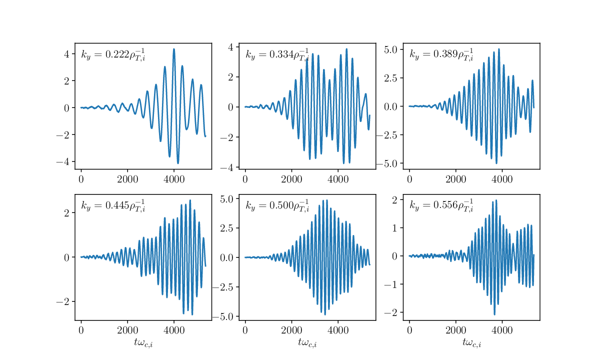

To illustrate the instability, the time history of the amplitude of density perturbation with different at are plotted in Fig. 4. We observe that all modes displayed grow initially, and saturate after . From the simulation data, the dispersion relation of the instability at can be calculated. It is plotted in Fig. 5.
After a sufficient long time, the unstable modes nonlinearly evolve into a turbulent state, as evident from the distribution of kinetic energy density and number density of ions at different times. Figure 6 shows that the kinetic energy diffuses as the instability grows, saturates, and becomes turbulent. Figure 7 shows that density blobs generated by the rupture of unstable modes are the prominent structures of the fully developed ITG turbulence. The details of the instability and turbulence, especially the formation of density blobs, can be observed from the video of the density evolution available at http://staff.ustc.edu.cn/˜xiaojy/ditg.html.
When turbulence develops, the energy or particle diffusion of the plasma across the magnetic field is conjectured empirically to follow the scaling of Bohm diffusion or the gyro-Bohm diffusion Taylor 1961; Drummond and Rosenbluth 1962; Waltz et al. 1990; Petty et al. 1995. The corresponding diffusion coefficients are
| (80) | |||||
| (81) |
where is the gyro-radius of ions measured in , the characteristic length of the plasma. Assuming that the diffusion coefficient varies slowly with and the energy density diffuses according to
| (82) |
we can calculate the numerical diffusion coefficient of ions in the -direction. The results are plotted in Fig. 8, where the local plasma characteristic length is estimated using
| (83) |
We observe that at the diffusion coefficient is between the Bohm scaling and gyro-Bohm scaling . Afterwards, decreases. When the ITG turbulence is fully developed at , the diffusion coefficient is closer to the gyro-Bohm scaling .
We emphasize again that simulating long-term dynamical and transport behavior of magnetized plasmas using fully kinetic particles demands a large number of simulation time-steps, in this case. A structure-preserving geometric algorithm with long-term accuracy and fidelity is desirable for this purpose. To verify the long-term conservative properties of the simulation, we plotted the energy error in Fig. 9. Clearly, the error is globally bounded by a small number for all simulation time-steps.


5 Discussion and Conclusion
In conclusion, we have customarily designed a field theory for low frequency electrostatic perturbations with fully kinetic ions and adiabatic electrons, and geometrically discretized the field theory to build a structure-preserving geometric PIC algorithm for simulating drift wave instabilities and turbulence in magnetized plasmas. The geometric discretization of the field theory is accomplished using DEC, high-order Whitney interpolation forms, and the non-canonical Hamiltonian splitting method. It preserves the non-canonical symplectic structure of the particle-field system, as well as the gauge symmetry. And as a result, the PIC algorithm is automatically charge-conserving and possesses long-term conservation properties that are indispensable for simulating the dynamics of fully kinetic particles. We have successfully implemented the algorithm in the SymPIC code. The algorithm was tested and benchmarked using the examples of ion Bernstein waves and drift waves, and applied to study the ion temperature gradient instability and turbulence in a 2D slab geometry. Simulation results show that at the early stage of the ITG turbulence, the energy diffusion is between the Bohm scaling and gyro-Bohm scaling. At later time, the observed diffusion is closer to the gyro-Bohm scaling, and density blobs generated by the rupture of unstable modes are the prominent structures of the fully developed ITG turbulence.
Acknowledgements.
This research was supported by the National Key Research and Development Program (2016YFA0400600, 2016YFA0400601 and 2016YFA0400602), the National Natural Science Foundation of China (NSFC-11775219 and NSFC-11575186), China Postdoctoral Science Foundation (2017LH002), the Fundamental Research Funds for the Central Universities (WK2030040096) and the U.S. Department of Energy (DE-AC02-09CH11466).References
- Krall and Rosenbluth (1965) N. A. Krall and M. N. Rosenbluth, Physics of Fluids 8, 1488 (1965).
- Coppi (1967) B. Coppi, Physics of Fluids 10, 582 (1967).
- Tang (1978) W. Tang, Nuclear Fusion 18, 1089 (1978).
- Horton (1999) W. Horton, Reviews of Modern Physics 71, 735 (1999).
- Dawson (1983) J. M. Dawson, Reviews of Modern Physics 55, 403 (1983).
- Hockney and Eastwood (1988) R. W. Hockney and J. W. Eastwood, Computer Simulation Using Particles (CRC Press, 1988).
- Birdsall and Langdon (1991) C. K. Birdsall and A. B. Langdon, Plasma Physics via Computer Simulation (IOP Publishing, 1991).
- Lee (1983) W. W. Lee, Physics of Fluids 26, 556 (1983).
- Dimits and Lee (1993) A. Dimits and W. W. Lee, Journal of Computational Physics 107, 309 (1993).
- Parker and Lee (1993) S. Parker and W. Lee, Physics of Fluids B: Plasma Physics 5, 77 (1993).
- Parker et al. (1993) S. Parker, W. Lee, and R. Santoro, Physical Review Letters 71, 2042 (1993).
- Hu and Krommes (1994) G. Hu and J. A. Krommes, Physics of Plasmas 1, 863 (1994).
- Dimits et al. (1996) A. Dimits, T. Williams, J. Byers, and B. Cohen, Physical Review Letters 77, 71 (1996).
- Lin et al. (1998) Z. Lin, T. S. Hahm, W. Lee, W. M. Tang, and R. B. White, Science 281, 1835 (1998).
- Parker et al. (1999) S. E. Parker, C. Kim, and Y. Chen, Physics of Plasmas 6, 1709 (1999).
- Frieman et al. (1966) E. A. Frieman, R. C. Davidson, and B. Langdon, Physics of Fluids 9, 1475 (1966).
- Catto (1978) P. J. Catto, Plasma Physics and Controlled Fusion 20, 719 (1978).
- Frieman and Chen (1982) E. Frieman and L. Chen, The Physics of Fluids 25, 502 (1982).
- Dubin et al. (1983) D. H. E. Dubin, J. A. Krommes, C. Oberman, and W. W. Lee, Physics of Fluids 26, 3524 (1983).
- Hahm (1988) T. S. Hahm, Physics of Fluids 31, 2670 (1988).
- Brizard (1989) A. Brizard, Journal of Plasma Physics 41, 541 (1989).
- Qin et al. (1998) H. Qin, W. M. Tang, and G. Rewoldt, Physics of Plasmas 5, 1035 (1998).
- Qin et al. (2000) H. Qin, W. M. Tang, and W. W. Lee, Physics of Plasmas 7, 4433 (2000).
- Qin and Tang (2004) H. Qin and W. M. Tang, Physics of Plasmas 11, 1052 (2004).
- Qin (2005) H. Qin, Fields Institute Communications 46, 171 (2005).
- Qin et al. (2007) H. Qin, R. Cohen, W. Nevins, and X. Xu, Physics of Plasmas 14, 056110 (2007).
- Burby (2015) J. W. Burby, Chasing Hamiltonian Structure in Gyrokinetic Theory, Ph.D. thesis, Princeton University (2015).
- Burby et al. (2015) J. Burby, A. Brizard, P. Morrison, and H. Qin, Physics Letters A 379, 2073 (2015).
- Wan and Parker (2012) S. Wan and Y. C. Parker, Phys. Rev. Lett 109, 185004 (2012).
- Wan et al. (2013) W. Wan, S. E. Parker, Y. Chen, R. J. Groebner, Z. Yan, A. Y. Pankin, and S. E. Kruger, Physics of Plasmas 20, 055902 (2013).
- Deng and Waltz (2015) Z. Deng and R. Waltz, Physics of Plasmas 22, 056101 (2015).
- Chen et al. (2008) Y. Chen, S. E. Parker, G. Rewoldt, S.-H. Ku, G.-Y. Park, and C.-S. Chang, Physics of Plasmas 15, 055905 (2008).
- Chowdhury et al. (2016) J. Chowdhury, Y. Chen, W. Wan, S. E. Parker, W. Guttenfelder, and J. Canik, Physics of Plasmas 23, 012513 (2016).
- Miecnikowski et al. (2018) M. T. Miecnikowski, B. J. Sturdevant, Y. Chen, and S. E. Parker, Physics of Plasmas 25, 055901 (2018).
- Sturdevant et al. (2017) B. Sturdevant, Y. Chen, and S. Parker, Physics of Plasmas 24, 081207 (2017).
- Hu et al. (2018) Y. Hu, M. Miecnikowski, Y. Chen, and S. Parker, Plasma 1, 105 (2018).
- Hirani (2003) A. N. Hirani, Discrete Exterior Calculus, Ph.D. thesis, California Institute of Technology (2003).
- (38) M. Desbrun, A. N. Hirani, M. Leok, and J. E. Marsden, http://arxiv.org/abs/math/0508341v2 .
- Whitney (1957) H. Whitney, Geometric Integration Theory (Princeton University Press, 1957).
- Squire et al. (2012a) J. Squire, H. Qin, and W. M. Tang, Geometric Integration of the Vlasov-Maxwell System with a Variational Particle-in-cell Scheme, Tech. Rep. PPPL-4748 (Princeton Plasma Physics Laboratory, 2012).
- Squire et al. (2012b) J. Squire, H. Qin, and W. M. Tang, Physics of Plasmas 19, 084501 (2012b).
- Xiao et al. (2015a) J. Xiao, H. Qin, J. Liu, Y. He, R. Zhang, and Y. Sun, Physics of Plasmas 22, 112504 (2015a).
- He et al. (2015a) Y. He, H. Qin, Y. Sun, J. Xiao, R. Zhang, and J. Liu, Physics of Plasmas 22, 124503 (2015a).
- He et al. (2017) Y. He, Z. Zhou, Y. Sun, J. Liu, and H. Qin, Physics Letters A 381, 568 (2017).
- Ruth (1983) R. D. Ruth, IEEE Transactions on Nuclear Science 30, 2669 (1983).
- Feng (1985) K. Feng, in the Proceedings of 1984 Beijing Symposium on Differential Geometry and Differential Equations, edited by K. Feng (Science Press, 1985) pp. 42–58.
- Feng (1986) K. Feng, Journal of Computational Mathematics 4, 279 (1986).
- Feng and Qin (2010) K. Feng and M. Qin, Symplectic Geometric Algorithms for Hamiltonian Systems (Springer, 2010).
- Forest and Ruth (1990) E. Forest and R. D. Ruth, Physica D 43, 105 (1990).
- Channell and Scovel (1990) P. J. Channell and C. Scovel, Nonlinearity 3, 231 (1990).
- Candy and Rozmus (1991) J. Candy and W. Rozmus, Journal of Computational Physics 92, 230 (1991).
- Hong and Qin (2002) J. Hong and M. Z. Qin, Applied Mathematics Letters 15, 1005 (2002).
- Tang (1993) Y.-F. Tang, Computers & Mathematics with Applications 25, 83 (1993).
- Shang (1994) Z. Shang, Journal of Computational Mathematics 2, 265 (1994).
- Shang (1999) Z. Shang, Numerische Mathematik 83, 477 (1999).
- Sanz-Serna and Calvo (1994) J. M. Sanz-Serna and M. P. Calvo, Numerical Hamiltonian Problems (Chapman and Hall, London, 1994).
- Marsden et al. (1998) J. E. Marsden, G. W. Patrick, and S. Shkoller, Communications in Mathematical Physics 199, 351 (1998).
- Sun and Qin (2000) Y. Sun and M. Qin, Journal of Mathematical Physics 41, 7854 (2000).
- Marsden and West (2001) J. E. Marsden and M. West, Acta Numer. 10, 357 (2001).
- Hairer et al. (2006) E. Hairer, C. Lubich, and G. Wanner, Geometric Numerical Integration: Structure-preserving Algorithms for Ordinary Differential Equations, Vol. 31 (Springer, 2006).
- Qin and Guan (2008) H. Qin and X. Guan, Physical Review Letters 100, 035006 (2008).
- Qin et al. (2009) H. Qin, X. Guan, and W. M. Tang, Physics of Plasmas 16, 042510 (2009).
- Zhang et al. (2014) R. Zhang, J. Liu, Y. Tang, H. Qin, J. Xiao, and B. Zhu, Physics of Plasmas 21, 032504 (2014).
- Ellison et al. (2015a) C. L. Ellison, J. M. Finn, H. Qin, and W. M. Tang, Plasma Physics and Controlled Fusion 57, 054007 (2015a).
- Burby and Ellison (2017) J. Burby and C. Ellison, Physics of Plasmas 24, 110703 (2017).
- (66) M. Kraus, http://arxiv.org/abs/1708.07356v1 .
- Ellison et al. (2018) C. L. Ellison, J. M. Finn, J. W. Burby, M. Kraus, H. Qin, and W. M. Tang, Physics of Plasmas 25, 052502 (2018).
- Ellison (2016) C. L. Ellison, Development of Multistep and Degenerate Variational Integrators for Applications in Plasma Physics, Ph.D. thesis, Princeton University (2016).
- Qin et al. (2013) H. Qin, S. Zhang, J. Xiao, J. Liu, Y. Sun, and W. M. Tang, Physics of Plasmas 20, 084503 (2013).
- He et al. (2015b) Y. He, Y. Sun, J. Liu, and H. Qin, Journal of Computational Physics 281, 135 (2015b).
- Zhang et al. (2015) R. Zhang, J. Liu, H. Qin, Y. Wang, Y. He, and Y. Sun, Physics of Plasmas 22, 044501 (2015).
- Ellison et al. (2015b) C. Ellison, J. Burby, and H. Qin, Journal of Computational Physics 301, 489 (2015b).
- Zhang et al. (2016) R. Zhang, H. Qin, Y. Tang, J. Liu, Y. He, and J. Xiao, Physical Review E 94, 013205 (2016).
- Wang et al. (2016) Y. Wang, J. Liu, and H. Qin, Physics of Plasmas 23, 122513 (2016).
- He et al. (2016a) Y. He, Y. Sun, J. Liu, and H. Qin, Journal of Computational Physics 305, 172 (2016a).
- Tu et al. (2016) X. Tu, B. Zhu, Y. Tang, H. Qin, J. Liu, and R. Zhang, Physics of Plasmas 23, 122514 (2016).
- Zhou et al. (2017) Z. Zhou, Y. He, Y. Sun, J. Liu, and H. Qin, Physics of Plasmas 24, 052507 (2017).
- (78) J. Xiao and H. Qin, http://arxiv.org/abs/1809.03697v1 .
- Shi et al. (2019) Y. Shi, Y. Sun, Y. He, H. Qin, and J. Liu, Numerical Algorithms (2019), 10.1007/s11075-018-0636-6.
- Xiao et al. (2013) J. Xiao, J. Liu, H. Qin, and Z. Yu, Physics of Plasmas 20, 102517 (2013).
- Evstatiev and Shadwick (2013) E. Evstatiev and B. Shadwick, Journal of Computational Physics 245, 376 (2013).
- Shadwick et al. (2014) B. A. Shadwick, A. B. Stamm, and E. G. Evstatiev, Physics of Plasmas 21, 055708 (2014).
- Xiao et al. (2015b) J. Xiao, J. Liu, H. Qin, Z. Yu, and N. Xiang, Physics of Plasmas 22, 092305 (2015b).
- Qin et al. (2016) H. Qin, J. Liu, J. Xiao, R. Zhang, Y. He, Y. Wang, Y. Sun, J. W. Burby, L. Ellison, and Y. Zhou, Nuclear Fusion 56, 014001 (2016).
- He et al. (2016b) Y. He, Y. Sun, H. Qin, and J. Liu, Physics of Plasmas 23, 092108 (2016b).
- Kraus et al. (2017) M. Kraus, K. Kormann, P. J. Morrison, and E. Sonnendrücker, Journal of Plasma Physics 83 (2017).
- Morrison (2017) P. J. Morrison, Physics of Plasmas 24, 055502 (2017).
- Xiao et al. (2017) J. Xiao, H. Qin, J. Liu, and R. Zhang, Physics of Plasmas 24, 062112 (2017).
- Xiao et al. (2018a) J. Xiao, H. Qin, and J. Liu, Plasma Science and Technology 20, 110501 (2018a).
- Xiao et al. (2018b) J. Xiao, H. Qin, Y. Shi, J. Liu, and R. Zhang, Physics Letters A (2018b), 10.1016/j.physleta.2018.12.010.
- Xiao et al. (2016) J. Xiao, H. Qin, P. J. Morrison, J. Liu, Z. Yu, R. Zhang, and Y. He, Physics of Plasmas 23, 112107 (2016).
- Zhou et al. (2014) Y. Zhou, H. Qin, J. Burby, and A. Bhattacharjee, Physics of Plasmas 21, 102109 (2014).
- Zhou et al. (2016) Y. Zhou, Y.-M. Huang, H. Qin, and A. Bhattacharjee, Physical Review E 93, 023205 (2016).
- Zhou (2017) Y. Zhou, Variational Integration for Ideal Magnetohydrodynamics and Formation of Current Singularities, Ph.D. thesis, Princeton University (2017).
- Chen et al. (2017) Q. Chen, H. Qin, J. Liu, J. Xiao, R. Zhang, Y. He, and Y. Wang, Journal of Computational Physics 349, 441 (2017).
- Shi et al. (2016) Y. Shi, N. J. Fisch, and H. Qin, Physical Review A 94, 012124 (2016).
- Shi et al. (2018) Y. Shi, J. Xiao, H. Qin, and N. J. Fisch, Physical Review E 97, 053206 (2018).
- Shi (2018) Y. Shi, Plasma Physics in Strong Field Regimes, Ph.D. thesis, Princeton University (2018).
- Yoshida (1990) H. Yoshida, Physics Letters A 150, 262 (1990).
- Fried and Conte (1968) B. D. Fried and S. D. Conte, The Plasma Dispersion Function (Academic Press, 1968).
- Romanelli (1989) F. Romanelli, Physics of Fluids B: Plasma Physics 1, 1018 (1989).
- Hammett and Perkins (1990) G. W. Hammett and F. W. Perkins, Physical Review Letters 64, 3019 (1990).
- Cowley et al. (1991) S. C. Cowley, R. Kulsrud, and R. Sudan, Physics of Fluids B: Plasma Physics 3, 2767 (1991).
- Dorland and Hammett (1993) W. Dorland and G. Hammett, Physics of Fluids B: Plasma Physics 5, 812 (1993).
- Rogers et al. (2000) B. N. Rogers, W. Dorland, and M. Kotschenreuther, Physical Review Letters 85, 5336 (2000).
- Dimits et al. (2007) A. Dimits, W. Nevins, D. Shumaker, G. Hammett, T. Dannert, F. Jenko, M. Pueschel, W. Dorland, S. Cowley, J. Leboeuf, T. Rhodes, J. Candy, and C. Estrada-Mila, Nuclear Fusion 47, 817 (2007).
- Ku et al. (2009) S. Ku, C. Chang, and P. Diamond, Nuclear Fusion 49, 115021 (2009).
- Merz and Jenko (2010) F. Merz and F. Jenko, Nuclear Fusion 50, 054005 (2010).
- Taylor (1961) J. Taylor, Physical Review Letters 6, 262 (1961).
- Drummond and Rosenbluth (1962) W. E. Drummond and M. N. Rosenbluth, The Physics of Fluids 5, 1507 (1962).
- Waltz et al. (1990) R. Waltz, J. DeBoo, and M. Rosenbluth, Physical Review Letters 65, 2390 (1990).
- Petty et al. (1995) C. Petty, T. Luce, K. Burrell, S. Chiu, J. Degrassie, C. Forest, P. Gohil, C. Greenfield, R. Groebner, R. Harvey, et al., Physics of Plasmas 2, 2342 (1995).