Finite-Time Influence Systems
and the Wisdom Of Crowd EffectThanks: Submitted to the editors DATE.

Francesco Bullo Email: bullo@engineering.ucsb.edu Thanks: Mechanical Engineering Department and the Center of Control, Dynamical-Systems and Computation, UC Santa Barbara, CA 93106-5070, USA. Fabio Fagnani Email: fabio.fagnani@polito.it Thanks: Department of Mathematical Sciences, Politecnico di Torino, Torino, Italy. Barbara Franci³³footnotemark: 3 Email: barbara.franci@polito.it. Thanks: Department of Mathematical Sciences, Politecnico di Torino, Torino, Italy.

Abstract

Recent contributions have studied how an influence system may affect the wisdom of crowd phenomenon. In the so-called naïve learning setting, a crowd of individuals holds opinions that are statistically independent estimates of an unknown parameter; the crowd is wise when the average opinion converges to the true parameter in the limit of infinitely many individuals. Unfortunately, even starting from wise initial opinions, a crowd subject to certain influence systems may lose its wisdom. It is of great interest to characterize when an influence system preserves the crowd wisdom effect.

In this paper we introduce and characterize numerous wisdom preservation properties of the basic French-DeGroot influence system model. Instead of requiring complete convergence to consensus as in the previous naïve learning model by Golub and Jackson, we study finite-time executions of the French-DeGroot influence process and establish in this novel context the notion of prominent families (as a group of individuals with outsize influence). Surprisingly, finite-time wisdom preservation of the influence system is strictly distinct from its infinite-time version. We provide a comprehensive treatment of various finite-time wisdom preservation notions, counterexamples to meaningful conjectures, and a complete characterization of equal-neighbor influence systems.

keywords

Opinion Dynamics, Influence System, Wisdom of Crowd, Learning

Funding.

This material is based upon work supported by, or in part by, the U.S. Army Research Laboratory and the U.S. Army Research Office under grant number W911NF-15-1-0577. This work has been done while Barbara Franci was a PhD Student sponsored by a TIM/Telecom Italia grant.

^†^†runningheads: Finite-Time Influence Systems
and the Wisdom Of Crowd Effect / Francesco Bullo, Fabio Fagnani and Barbara Franci

1 Introduction

Problem description and motivation. Social scientists describe as wisdom of crowds the phenomenon whereby large groups of people are collectively smarter than single individuals. Much research has focused on understanding the conditions under which such a phenomenon occurs. It is generally assumed that required conditions include diversity of opinions, independence of opinions, and a system that aggregates individual opinions without introducing bias. Indeed, one plausible explanation for this phenomenon in certain estimation tasks is that: (i) each individual opinion is influenced by an independent zero-mean noise and, therefore, (ii) taking averages of large numbers of individual opinions will reduce the effect of noise.

A natural system that aggregates individual opinions is an influence system, that is, a social dynamic process whereby individual opinions, starting from their respective initial conditions, evolve possibly towards consensus. So it is natural to study the conditions under which an influence system enhances, preserves, or diminishes the wisdom of crowd effect. Motivated precisely by such reasoning, an insightful naïve learning model was recently proposed by Golub and Jackson [15]. In this model, initial individual opinions are measurements of an unknown parameter corrupted by independent zero-mean noise. The law of large numbers then says that the crowd is initially wise, in the sense that the average initial opinion equals the unknown parameter in the limit of infinitely many individuals. Moreover, and more relevant here, the social influence process is wisdom preserving if, starting from wise individual estimates, the crowd remains wise after the execution of the influence process. In other words, the influence system is wisdom preserving if its execution does not introduce bias in the crowd’s estimate of the unknown parameter.

This paper is a contribution to the naïve learning model; instead of requiring that the opinion formation process is allowed infinite time in order for the crowd to reach consensus, we here investigate the more realistic setting in which the influence system is executed only for finite time. Accordingly, we investigate the finite-time wisdom preservation properties of the influence system. For such finite-time settings, we aim to define a number of wisdom notions, provide rigorous characterizations, and work out instructive examples. In what follows, in the interest of brevity and consistency with the original work [15], we refer to a wisdom preserving influence system as a wise influence system.

Literature review. Aristotle is thought to be the first author to write about the “wisdom of the crowd” in his work “Politics.” Galton [14] describes a famous classic experiment concerning the weight of a slaughtered ox and documents how the average estimate of the ox’s weight was indeed remarkably close to its correct value. In recent years, Surowiecki’s book [23] has widely popularized the concept and discussed potential applications to group decision making and forecasting.

The literature on opinion dynamics and influence systems is very rich. The classic and widely-established French-DeGroot averaging model is discussed in the text on influence systems by Friedkin and Johnsen [13], the text on social networks by Jackson [16], and the recent survey by Proskurnikov and Tempo [21]. Inextricably linked with influence systems is the concept of centrality in its various incarnations. Especially relevant to this work is the notion of the eigenvector centrality, e.g., see the foundational works by Bonacich [6] and Friedkin [12]. [8] provides a bounded rational interpretation, a low-rank property, and the asymptotic behavior over reducible graphs of the French-DeGroot averaging model. The phenomenon of wisdom of crowds is related also to the topic of social learning. We refer to the original work [15] for a insightful comparison between the naïve learning approach and other distinct methods. We here only outline two alternative approaches. First, Acemoglu et al [2] present a game-theoretical model for sequential learning; even in this setup the presence of “excessively influential agents” is an impediment to social learning. Second, the social learning model proposed by Jadbabaie et al [17] is based on the constant arrival of new information (i.e., a feature our model does not have) and shows that new information together with basic connectivity properties is sufficient to overcome the influence of any individual agent.

The understanding of what social influence processes do indeed enhance or diminishes the wisdom of a crowd continues to be of very recent interest and debate. Lorenz et al [19] describe an empirical study in which the influence system diminishes the accuracy of the collective estimate by diminishing diversity of the crowd (even while conducing the opinions closer to consensus). In contrast, Becker et al [4] present theoretical and empirical evidence about settings in which the influence system enhances the wisdom of the crowd.

Contributions. We start by reviewing the naïve learning model for large populations proposed by Golub and Jackson [15] and based on the French-DeGroot opinion formation process. In this model, the population is wise if the final (in the limit as time $k\to\infty$ ) consensus opinion is equal to the correct value. This property is cast in terms of the left dominant eigenvector of the influence matrix in large populations (i.e., in the limit as the number of individual $n\to\infty$ ). Specifically, a wise population is a sequences of row-stochastic matrices whose left dominant eigenvector satisfies a “vanishing maximum entry condition.” This condition ensures that no individual’s initial erroneous opinion has an outside impact on the final consensus opinion, thereby rendering the population unwise.

In this paper we consider a variation of the naïve learning setting in which the French-DeGroot opinion formation process is allowed only finite time and does not, therefore, reach completion. Our individuals do not reach consensus and, in this paper, a population is finite-time wise if the average of the individuals opinion remains correct as time progresses along the opinion dynamics process. In other words, [15] considers wisdom in the limit in which $n\to\infty$ after $k\to\infty$ , we here consider the limit in which $n\to\infty$ after at $k=1$ , $k$ fixed, and uniformly over $k$ . We argue that these finite-time variations are especially relevant for large population, since it is known that the time required for consensus to be approximately achieved typically diverges as the population size diverges. Note that even controlled experiments are executed with a finite time constraint, e.g., see the recent work in [4] where $k$ is precisely equal to 2. It is therefore of interest to assume that no enough time is provided to the opinion formation process to achieve complete consensus and inquire what are wise sequences under this relaxed condition.

Given this premise, this paper makes four main contributions. First, for our proposed finite-time setting we introduce the notions of one-time wisdom, finite-time wisdom, uniform wisdom, and pre-uniform wisdom. We provide necessary and sufficient characterizations of one-time and finite-time wisdom in terms of the limiting value of the maximum column averages of the matrix sequence. We also provide a sufficient condition for uniform wisdom involving the same limiting value as well as the limiting value of the matrices’ mixing time.

Second, we provide numerous detailed examples of graph families to establish, among other relationships, that finite-time wisdom neither implies nor is implied by wisdom, as previously defined. Our examples illustrate how various general implications among the various wisdom notions are tight. Our examples also demonstrate that the proposed notions of one-time and finite-time wisdom are meaningful and strictly distinct from the notion of (infinite-time) wisdom as defined by Golub and Jackson [15].

Third, we provide a sufficient condition to ensure that a sequence of row-stochastic matrices is indeed finite-time wise. We introduce an appropriate novel notion of prominent family and show how its absence implies finite-time wisdom in general. Roughly speaking, a collection of nodes (a family) is prominent if, in the limit of large population, its size is negligible (that is, of order $o(n)$ ) but its total accorded one-time influence is not (that is, of order 1 in $n$ ).

Fourth, we then extend our sufficient condition to the setting of equal-neighbor sequences of row-stochastic matrices. For such highly-structured case, we show that the absence of prominent individuals is a necessary and sufficient condition for finite-time wisdom, pre-uniform wisdom, and wisdom in the equal-neighbor setting. In other words, we completely characterize finite-time wisdom in the equal-neighbor setting. We apply these findings to the case of preferential attachment model and show how (1) the classic Barabási-Albert model (with attachment probability linearly proportional to degree) is wise in all possible senses (finite-time, uniformly and infinite-time), whereas (2) a super-linear preferential attachment model loses all its wisdom properties.

Paper organization. Section 2 contains various wisdom definitions and corresponding general conditions. Section 3 contains the analysis of several counterexamples showing the general difference among the various wisdom notions. Section 4 contains a sufficient condition for finite-time wisdom and Section 5 characterizes pre-uniform wisdom in sequences of equal-neighbor matrices. Section 6 contains some concluding remarks.

1.1 Review of notation and preliminary concepts

Let $\mathbbold{1}_{n}\in\mathbb{R}^{n\times 1}$ denote the vector of all ones. Given $x\in\mathbb{R}^{n}$ , we define its average by $\ave(x)=\frac{1}{n}\mathbbold{1}_{n}^{\top}x=\frac{1}{n}\sum_{i=1}^{n}x_{i}$ . Given $x\in\mathbb{R}^{n}$ , its norms by $\|x\|_{1}=\sum_{i}|x_{i}|$ , $\|x\|_{2}=(\sum_{i}x_{i}^{2})^{1/2}$ and $\|x\|_{\infty}=\max_{i}|x_{i}|$ . Let $\Delta_{n}=\{x\in\mathbb{R}^{n}\;|\;x\geq 0,\mathbbold{1}_{n}^{\top}{x}=1\}$ . Given $x\in\Delta_{n}$ , the following inequalities hold

\|x\|_{\infty}^{2}\leq x^{\top}x\leq\|x\|_{\infty}.

(1)

Indeed, the left-hand side is self evident, while right-hand side follows from $x^{\top}x\leq\|x\|_{\infty}\|x\|_{1}=\|x\|_{\infty}$ .

Stochastic matrices. A matrix $P\in\mathbb{R}^{n\times{n}}$ is non-negative ( $P\geq 0$ ) if $P_{ij}\geq 0$ for each $i,j$ . For such a matrix, the maximum column sum is

\|P\|_{1}=\max_{j\in\{1,\dots,n\}}\sum_{i=1}^{n}P_{ij}=\max\mathbbold{1}_{n}^{\top}P.

Note that $\|\frac{1}{n}P\|_{1}$ is the maximum column average of $P$ . To a nonnegative matrix $P$ we associate an unweighted directed graph $G=(\{1,\dots,n\},E)$ where $E=\{(i,j)\in\{1,\dots,n\}^{2}\;|\;P_{ij}>0\}$ . Given a node $j$ , let $N_{j}$ denote the set of out-neighbors of $j$ . The nonnegative matrix $P$ is irreducible if $G$ is strongly connected and primitive if $G$ is strongly connected and aperiodic.

A matrix $P\in\mathbb{R}^{n\times{n}}$ is stochastic if $P\geq 0$ and $P\mathbbold{1}_{n}=\mathbbold{1}_{n}$ .

Given a stochastic irreducible matrix $P$ , its left dominant eigenvector $\pi\in\Delta_{n}$ is unique and well defined by the Perron-Frobenius Theorem and satisfies $\pi^{\top}P=\pi^{\top}$ .

Given a primitive stochastic matrix $P$ , its mixing time is defined by

\tau_{\textup{mix}}(P):=\inf\Big\{t\in\mathbb{N}\;\Big|\;\max_{i,j}\sum\nolimits_{k}|(P)^{t}_{ik}-P)^{t}_{jk}|\leq\frac{1}{\textrm{e}}\Big\}\,.

(2)

Equal-neighbor models.

Definition 1 (Equal-neighbor, directed equal-neighbor, and weighted-neighbor matrices).

Given a nonnegative matrix $W\in\mathbb{R}_{\geq 0}^{n\times{n}}$ with at least one positive entry in each row (possibly on the diagonal), define the stochastic matrix $P\in\mathbb{R}^{n\times{n}}$ by

P=\diag(W\mathbbold{1}_{n})^{-1}W.

(3)

Then the matrix $P$ is said to be

(i)

equal-neighbor if all non-zero entries of $W$ have the same value and $W=W^{\top}$ ,
(ii)

directed equal-neighbor if all non-zero entries of $W$ have the same value and $W\neq W^{\top}$ , and
(iii)

weighted-neighbor if the non-zero entries of $W$ take more than one value and $W=W^{\top}$ .

In these three definitions, the graph associated to $W$ is undirected unweighted, directed unweighted, and undirected weighted respectively.

Note that, given a non-negative weight matrix $W\in\mathbb{R}_{\geq 0}^{n\times{n}}$ , the weighted out-degree of a node $i$ in the weighted digraph associated to $W$ is $d_{i}=(W\mathbbold{1}_{n})_{i}=\sum_{j=1}^{n}W_{ij}$ . Because we assume $d_{i}>0$ for all $i$ , equation (3) is well-posed and equivalent to:

P_{ij}=d_{i}^{-1}W_{ij}.

If $W$ is symmetric, then $d_{i}$ is called the weighted degree. If additionally $W$ is binary, then $d_{i}$ is called the degree and

P_{ij}=d_{i}^{-1}W_{ij}=\begin{cases}d_{i}^{-1},\qquad&\text{if }j\in N_{i},\\ 0,&\text{otherwise }.\end{cases}

(4)

We conclude with a known useful result. The left dominant eigenvector $\pi$ of an irreducible weighted-neighbor matrix $P$ satisfies, for all $i\in\{1,\dots,n\}$ ,

\pi_{i}=\frac{d_{i}}{d_{1}+\dots+d_{n}}.

(5)

2 Wisdom in sequences of stochastic matrices: definitions and basic results

We consider the classic French-DeGroot model [11, 7] of opinion dynamics

x_{i}(k+1)=\sum_{j=1}^{n}P_{ij}x_{j}(k),

(6)

where $x_{i}(k)$ denotes the opinion of individual $i$ , $i\in\{1,\dots,n\}$ at time $k\in\mathbb{Z}_{\geq 0}$ . The coefficient $P_{ij}$ denotes the weight that individual $i$ assigns to individual $j$ when carrying out this revision. The matrix $P$ is assumed row-stochastic and defines a weighted directed graph $G$ .

We assume

x_{i}(0)=\mu+\xi_{i}(0),

(7)

where the constant $\mu\in\mathbb{R}$ is unknown parameter and the noisy terms $\xi_{i}(0)$ are a family of independent Gaussian-distributed variables such that $\EE[\xi_{i}(0)]=0$ and $\Var[\xi_{i}(0)]=\sigma^{2}<\infty$ for all $i\in\{1,\dots,n\}$ .

We will consider sequences of DeGroot models (6) with increasing dimensions $n$ and denote all relative quantities with a superscript $[n]$ . In particular, the state of the $n$ -dimensional model is $x^{[n]}$ . Given assumption (7) and assuming $\mu$ is kept constant, the law of large numbers implies that, almost surely,

\lim_{n\to\infty}\ave(x^{[n]}(0)))=\mu.

Definition 2 (Wisdom notions).

Given a sequence of stochastic matrices of increasing dimensions $\{P^{[n]}\in\mathbb{R}^{n\times{n}}\}_{n\in\mathbb{N}}$ , define a sequence of opinion dynamics problems with initial state $\{x^{[n]}(0)\in\mathbb{R}^{n}\}_{n\in\mathbb{N}}$ satisfying assumption (7) and evolution $\{x^{[n]}(k)\in\mathbb{R}^{n}\}_{n\in\mathbb{N}}$ at times $k\in\mathbb{N}$ . The sequence $\{P^{[n]}\in\mathbb{R}^{n\times{n}}\}_{n\in\mathbb{N}}$ , is

(i)

one-time wise if $\lim\limits_{n\to\infty}\ave(x^{[n]}(1)))=\mu$ ;
(ii)

finite-time wise if $\lim\limits_{n\to\infty}\ave(x^{[n]}(k)))=\mu$ , for all $k\in\mathbb{N}$ ;
(iii)

wise if $\lim\limits_{n\to\infty}\lim\limits_{k\to\infty}\ave(x^{[n]}(k)))=\mu$ ;
(iv)

uniformly wise if $\lim\limits_{n\to\infty}\sup\limits_{k\in\mathbb{N}}|\ave(x^{[n]}(k)))-\mu|=0$ .

Here all limits are meant in the probability sense.

The terminology “wisdom preserving” instead of “wise” would be more appropriate in this context. Indeed, we here study whether the dynamics driven by the matrices $P^{[n]}$ preserves or diminishes the crowd’s wisdom assumed to hold at initial time. As already remarked in the Introduction, we have chosen this simpler name in the interest of brevity and consistency with the original work [15].

We note two straightforward relations among these notions of wisdom, that is, (ii) implies (i) and (iv) implies (iii). More details on such implications are given in Section 3.

The following theorem provides necessary and sufficient characterizations of the notions (i), (ii), and (iii) of the above definition. The proof of these characterizations is immediate from [15, 22].

Theorem 3 (Necessary and sufficient conditions for finite-time wisdom and wisdom).

Consider a sequence of stochastic matrices of increasing dimensions $\{P^{[n]}\in\mathbb{R}^{n\times{n}}\}_{n\in\mathbb{N}}$ . The sequence is

(i)

one-time wise if and only if $\lim\limits_{n\to\infty}\|\frac{1}{n}P^{[n]}\|_{1}=0$ ;
(ii)

finite-time wise if and only if, for all $k\in\mathbb{N}$ , $\lim\limits_{n\to\infty}\|\frac{1}{n}(P^{[n]})^{k}\|_{1}=0$ .

Moreover, assuming $\{P^{[n]}\}_{n\in\mathbb{N}}$ are primitive, the sequence is

(iii)

wise if and only if $\lim\limits_{n\to\infty}\|\pi^{[n]}\|_{\infty}=0$ , where $\pi^{[n]}\in\Delta_{n}$ is the left dominant eigenvector of $P^{[n]}$ , for $n\in\mathbb{N}$ .

Proof.

Define

\chi^{[n]}(k)=\frac{1}{n}\mathbbold{1}_{n}^{\top}(P^{[n]})^{k}

(8)

and notice that

\ave(x^{[n]}(k))=\mu+(\chi^{[n]}(k))^{\top}\xi^{[n]}(0).

Thus,

	$\displaystyle\EE[\ave(x^{[n]}(k))]$	$\displaystyle=\mu,$		(9)
	$\displaystyle\Var[\ave(x^{[n]}(k))]$	$\displaystyle=\sigma^{2}(\chi^{[n]}(k))^{\top}\chi^{[n]}(k).$		(10)

By Chebyshev’s inequality, the convergence in probability of $\ave(x^{[n]}(k))$ to $\mu$ is equivalent to the convergence to $0$ of the variance. Statements (i) and (ii) can now be proven by applying the inequalities (1) with $x=\chi^{[n]}(k)$ and noting that $\|\chi^{[n]}(k)\|_{\infty}=\|\frac{1}{n}(P^{[n]})^{k}\|_{1}$ .

Regarding statement (iii), the primitivity assumption implies $\lim\limits_{k\to+\infty}x^{[n]}(k)=(\pi^{[n]})^{\top}\big(\mu\mathbbold{1}_{n}+\xi^{[n]}(0)\big)\mathbbold{1}_{n}$ where $\pi^{[n]}$ is the left dominant eigenvector of $P^{[n]}$ . Therefore,

\lim\limits_{k\to+\infty}\ave(x^{[n]}(k))=\mu+(\pi^{[n]})^{\top}\xi^{[n]}(0),

and statement (iii) follows by applying the inequalities (1) with $x=\pi^{[n]}$ .

Remark 4 (Estimation theory interpretation).

Adopting statistics language, our paper is concerned with the properties of the arithmetic average estimator $x\mapsto\sum_{i=1}^{n}x_{i}/n$ applied to the stochastic process $\{x^{[n]}(k)\}_{k\in\mathbb{N}}$ . Equation (9) implies that, for every $n$ and for every $k$ , the arithmetic average estimator, regarded as a random variable, is unbiased. We are interested in concentration results, that is, we investigate when, as $k$ varies and as $n\to+\infty$ , the estimator has its variance converging to $0$ , namely, when the estimator concentrates around its mean value.

There is a natural property that, in analogy to the other characterizations presented in Theorem 3, is related to uniform wisdom. We present it as a separated concept.

Definition 5 (Pre-uniform wisdom).

A sequence of stochastic matrices of increasing dimensions $\{P^{[n]}\in\mathbb{R}^{n\times{n}}\}_{n\in\mathbb{N}}$ is pre-uniformly wise if $\lim\limits_{n\to\infty}\sup\limits_{k\in\mathbb{N}}\|\frac{1}{n}(P^{[n]})^{k}\|_{1}=0$ .

While pre-uniform wisdom is not sufficient to guarantee uniform wisdom, it surely yields wisdom and finite-time wisdom, as an immediate consequence of Theorem 3.

Finally, for what concerns uniform wisdom, we present a sufficient condition that turns out to be useful in many applications. Recall the notion of mixing time from equation (2).

Theorem 6 (A sufficient condition for uniform wisdom).

A sequence of primitive stochastic matrices of increasing dimensions $\{P^{[n]}\in\mathbb{R}^{n\times{n}}\}_{n\in\mathbb{N}}$ is uniformly wise if

\lim\limits_{n\to+\infty}\sup\limits_{k\in\mathbb{N}}\Big\|\frac{1}{n}(P^{[n]})^{k}\Big\|_{1}\tau_{\textup{mix}}(P^{[n]})=0.

Proof.

Define

Y^{[n]}(k)=\ave(x^{[n]}(k)))-\mu=\chi^{[n]}(k)^{\top}\xi^{[n]}(0),

where $\chi^{[n]}(k)$ is defined in (8). Notice that

\lim\limits_{k\to+\infty}Y^{[n]}(k)=Y^{[n]}:=(\pi^{[n]})^{\top}\xi^{[n]}(0).

Fix $\delta>0$ and notice that

\Prob\!\Big[\sup\limits_{k\in\mathbb{N}}|Y^{[n]}(k)|>\delta\Big]\leq\Prob\!\Big[\sup\limits_{k\in\mathbb{N}}|Y^{[n]}(k)-Y^{[n]}|>\delta/2\Big]+\Prob[|Y^{[n]}|>\delta/2].

(11)

We now estimate the two right-end-side terms of equation (11). Regarding the first term, we fix $k$ and we use Chebyshev’s inequality to obtain

$\displaystyle\Prob[\|Y^{[n]}(k)-Y^{[n]}\|>\delta/2]$	$\displaystyle\leq\frac{4}{\delta^{2}}\Var[Y^{[n]}(k)-Y^{[n]}]$
	$\displaystyle\leq\frac{4}{\delta^{2}}(\chi^{[n]}(k)-\pi^{[n]})^{\top}(\chi^{[n]}(k)-\pi^{[n]})$
	$\displaystyle\leq\frac{4}{\delta^{2}}\\|\chi^{[n]}(k)-\pi^{[n]}\\|_{\infty}\\|\chi^{[n]}(k)-\pi^{[n]}\\|_{1}$	(12)

Since $\|\chi^{[n]}(k)\|_{\infty}=\|\frac{1}{n}(P^{[n]})^{k}\|_{1}$ and $\chi^{[n]}(k)\to\pi^{[n]}$ for $k\to+\infty$ , the $\infty$ -norm factor can be estimated as

\|\chi^{[n]}(k)-\pi^{[n]}\|_{\infty}\leq\|\chi^{[n]}(k)\|_{\infty}+\|\pi^{[n]}\|_{\infty}\leq 2\sup\limits_{k\in\mathbb{N}}\Big\|\frac{1}{n}(P^{[n]})^{k}\Big\|_{1}.

(13)

The final $1$ -norm factor in equation (12) can be estimated in terms of the mixing time [18, Section 4.5]

\|\chi^{[n]}(k)-\pi^{[n]}\|_{1}\leq\exp\left(-\left\lfloor\frac{k}{\tau_{\textup{mix}}(P^{[n]})}\right\rfloor\right).

(14)

Substituting (13) and (14) into inequality (12) and using a union bound estimation (also referred to as Boole’s inequality), we now obtain

$\displaystyle\Prob\!\Big[\sup\limits_{k\in\mathbb{N}}\|Y^{[n]}(k)-Y^{[n]}\|>\delta/2\Big]$	$\displaystyle\leq\frac{8}{\delta^{2}}\sup\limits_{k\in\mathbb{N}}\Big\\|\frac{1}{n}(P^{[n]})^{k}\Big\\|_{1}\sum_{k}\exp\left(-\left\lfloor\frac{k}{\tau_{\textup{mix}}(P^{[n]})}\right\rfloor\right)$
	$\displaystyle=\frac{8e}{\delta^{2}}\sup\limits_{k\in\mathbb{N}}\Big\\|\frac{1}{n}(P^{[n]})^{k}\Big\\|_{1}\frac{1}{1-\exp\left(-\frac{1}{\tau_{\textup{mix}}(P^{[n]})}\right)}$
	$\displaystyle\leq\frac{8e}{\delta^{2}}\sup\limits_{k\in\mathbb{N}}\Big\\|\frac{1}{n}(P^{[n]})^{k}\Big\\|_{1}\tau_{\textup{mix}}(P^{[n]}).$	(15)

The second term in the right-hand-side of equation (11) can be easily bounded using Chebyshev’s inequality and the simple bound (1):

$\displaystyle\Prob[\|Y^{[n]}\|>\delta/2]$	$\displaystyle\leq\frac{4}{\delta^{2}}\Var[Y^{[n]}]=\frac{4}{\delta^{2}}(\pi^{[n]})^{\top}(\pi^{[n]})$
	$\displaystyle\leq\frac{4}{\delta^{2}}\\|\pi^{[n]}\\|_{\infty}$
	$\displaystyle\leq\frac{4}{\delta^{2}}\sup\limits_{k\in\mathbb{N}}\Big\\|\frac{1}{n}(P^{[n]})^{k}\Big\\|_{1}.$	(16)

The theorem statement follows from putting together the inequalities (11), (15), and (16).

3 Basic implications and counterexamples

In the following lemma we show how the basic wisdom notions in Definitions 2 and 5 are related by a simple implication and how four counterexamples show that no additional statements may be made in general. To construct our counterexamples, we will rely upon the equal neighbor models as in Definition 1.

Lemma 7 (Basic implications and counterexamples).

If a sequence of primitive stochastic matrices of increasing dimensions $\{P^{[n]}\in\mathbb{R}^{n\times{n}}\}_{n\in\mathbb{N}}$ is uniformly wise or pre-uniformly wise, then it is wise and finite-time wise. Moreover, there exist sequences that

(i)

are neither wise nor finite-time wise (see Example 1),
(ii)

are wise, but not one-time wise (see Example 2),
(iii)

are finite-time wise, but not wise (see Example 3), and
(iv)

are wise and finite-time wise, but not pre-uniformly wise (see Example 4).

We illustrate this lemma in Figure 1. The proof of the first statement in the lemma is an immediate consequence of Definition 5 and the characterizations in Theorem 3. The four existence statement are established by providing explicit examples here below.

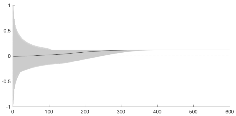
Each example includes a figure illustrating a numerical simulation of the corresponding dynamics. In the simulations the initial opinions are independently normally distributed with zero mean and unit standard deviation, except for $x^{[n]}_{1}(0)=1$ (for illustration purposes).

Figure 1: Logical relations among sets of sequences with varying degree of wisdom. For each set we provide an example sequence that belongs to that set, but not to any strict subset of it.

Example 1 (The star graph is neither wise nor finite-time wise).

For $n\in\mathbb{N}$ , define $\{P^{[n]}\in\mathbb{R}^{n\times{n}}\}_{n\in\mathbb{N}}$ by

\displaystyle P^{[n]}=\begin{bmatrix}1/n&1/n&1/n&\cdots&1/n\\ 1&0&0&\vdots&0\\ 1&0&0&\vdots&0\\ \vdots&\vdots&\vdots&\ddots&\vdots\\ 1&0&0&\cdots&0\end{bmatrix}.

In other words, consider the sequence of primitive equal-neighbor matrices defined by increasing-dimension star graphs (with a self-loop at the central node). It is easy to see that the dominant left eigenvector of $P^{[n]}$ is $\pi^{[n]}=\begin{bmatrix}\frac{n}{2n-1}&\frac{1}{(2n-1)}&\dots&\frac{1}{(2n-1)}\end{bmatrix}^{\top}$ . The sequence $\{P^{[n]}\}_{n\in\mathbb{N}}$ is neither wise, nor one-time wise because

	$\displaystyle\lim_{n\to\infty}\\|\pi^{[n]}\\|_{\infty}$	$\displaystyle=\lim_{n\to\infty}\pi_{1}^{[n]}=\frac{1}{2},$
	$\displaystyle\lim_{n\to\infty}\\|\tfrac{1}{n}P^{[n]}\\|_{1}$	$\displaystyle=\lim_{n\to\infty}\max_{j\in\{1,\dots,n\}}\frac{1}{n}\sum_{i=1}^{n}P^{[n]}_{ij}$
		$\displaystyle=\lim_{n\to\infty}\frac{1}{n}\sum_{i=1}^{n}P^{[n]}_{i1}=\lim_{n\to\infty}\frac{n-1+1/n}{n}=1.$

The lack of wisdom and finite-time wisdom is illustrated in Figure 2. $\square$

Refer to caption — Figure 2: Star graph with $n=100$ nodes (one root and $99$ leaves). The time horizon is $T=600$ . Individual opinions are in gray, the average opinion is in black. As proved in Example 1, the figure illustrates how the graph is neither wise nor finite-time wise.

Example 2 (The union/contraction of star and complete graph is wise, but not one-time wise).

For $n\in\mathbb{N}$ , let $S_{n}\sqcup K_{n}$ denote the undirected graph with $2n$ nodes obtained by (i) computing the union of the star $S_{n}$ (one center node and $n$ leafs) and a complete graph $K_{n}$ , and (ii) identifying/contracting one leaf of $S_{n}$ with a node of $K_{n}$ . Accordingly, let $\{W^{[n]}\}_{n\in\mathbb{N}}$ be the sequence of adjacency matrices of $\{S_{n}\sqcup K_{n}\}_{n\in\mathbb{N}}$ and $\{P^{[n]}\}_{n\in\mathbb{N}}$ be the corresponding sequence of equal-neighbor matrices. These matrices are primitive because $K_{n}$ contains cycles with co-prime length. Note the slight abuse of notation: $P^{[n]}$ has dimension $2n$ .

The graph $S_{n}\sqcup K_{n}$ , for $n=6$ , is depicted in Figure 3, where nodes are numbered as follows: node $1$ is always the center of the star and node $n+1$ is the node belonging to both the star and the complete graph.

Figure 3: The union and contraction of a star graph with a complete graph.

For this graph $S_{n}\sqcup K_{n}$ , from equation (5), we compute the left dominant eigenvector of $P^{[n]}$ . First, we observe that: $d_{1}=n$ , $d_{j}=1$ for a generic leaf $j\in\{2,\dots,n\}$ , $d_{n+1}=n$ , and $d_{h}=n-1$ a generic node $h\in\{n+2,\dots,2n\}$ in $K_{n}$ . Hence, the sum of all degrees is $n+1\cdot(n-1)+n+(n-1)^{2}=n^{2}+n$ and the left dominant eigenvector satisfies:

	$\displaystyle\pi^{[n]}_{1}=\frac{n}{n^{2}+n},\kern 5.0pt\pi^{[n]}_{j}=\frac{1}{n^{2}+n},$
	$\displaystyle\pi^{[n]}_{n+1}=\frac{n}{n^{2}+n},\kern 5.0pt\pi^{[n]}_{h}=\frac{n-1}{n^{2}+n}.$

Next, we compute the column sums of $P^{[n]}$ . For the two special nodes we have

	$\displaystyle\sum_{i=1}^{2n}P^{[n]}_{i1}$	$\displaystyle=\sum_{i=2}^{n}P^{[n]}_{i1}+P^{[n]}_{n+1,1}=(n-1)+\frac{1}{n},$
	$\displaystyle\sum_{i=1}^{2n}P^{[n]}_{i,n+1}$	$\displaystyle=P^{[n]}_{1,n+1}+\sum_{i=n+2}^{2n}P^{[n]}_{i,n+1}=1+\frac{1}{n},$

and, for a generic leaf $j\in\{2,\dots,n\}$ in $S_{n}$ and a generic $h\in\{n+2,\dots,2n\}$ in $K_{n}$ , we have

	$\displaystyle\sum_{i=1}^{2n}P^{[n]}_{ij}$	$\displaystyle=\frac{1}{n},$
	$\displaystyle\sum_{i=1}^{2n}P^{[n]}_{ih}$	$\displaystyle=P^{[n]}_{n+1,h}+\sum_{i=n+2}^{2n}P^{[n]}_{ih}=\frac{1}{n}+(n-2)\frac{1}{n-1}.$

In summary, we note that the sequence $\{P^{[n]}\}_{n\in\mathbb{N}}$ is wise but not one-time wise because

	$\displaystyle\lim_{n\to\infty}\\|\pi^{[n]}\\|_{\infty}$	$\displaystyle=\lim_{n\to\infty}\pi_{1}^{[n]}=\lim_{n\to\infty}\frac{n}{n^{2}+n}=0,$
	$\displaystyle\lim_{n\to\infty}\\|\tfrac{1}{2n}P^{[n]}\\|_{1}$	$\displaystyle=\lim_{n\to\infty}\max_{j\in\{1,\dots,2n\}}\frac{1}{2n}\sum_{i=1}^{2n}P^{[n]}_{ij}$
		$\displaystyle=\lim_{n\to\infty}\frac{1}{2n}\sum_{i=1}^{2n}P^{[n]}_{i1}=\lim_{n\to\infty}\frac{n-1+\frac{1}{n}}{2n}=\frac{1}{2}.$

The lack of one-time wisdom and the presence of wisdom is illustrated in Figure 4. $\square$

Example 3 (The path graph with biased weights is finite-time wise, but not wise).

Consider a sequence of increasing-dimension path graphs whose biased weights are selected as follows: (i) pick a constant $\nu>1$ and define the unique scalars $q>p>0$ satisfying $q/p=\nu$ and $p+q=1$ , and (ii) define the $n$ -dimensional weighted digraph as in Figure 5 (self-loops at node $1$ and $n$ ). Let $\{P^{[n]}\}_{n\in\mathbb{N}}$ denote the sequence of primitive stochastic adjacency matrices of the the path graphs with biased weights. We have:

Figure 5: Directed path with biased weights

\displaystyle P^{[n]}=\begin{bmatrix}p&q&\cdots&0&0\\ p&0&q&\ddots&0\\ \vdots&\ddots&\ddots&\ddots&0\\ 0&\ddots&p&0&q\\ 0&0&\cdots&p&q\end{bmatrix}.

Let $\pi^{[n]}$ be the dominant left eigenvector of $P^{[n]}$ . We claim that

\pi^{[n]}_{1}=\frac{\nu-1}{\nu^{n}-1},\qquad\pi^{[n]}_{i}=\nu^{i-1}\pi^{[n]}_{1},\text{ for $i\in\{2,\dots,n\}$}.

(17)

We prove this claim as follows. From $(\pi^{[n]})^{\top}=(\pi^{[n]})^{\top}P^{[n]}$ , we get

	$\displaystyle\pi^{[n]}_{1}p+\pi^{[n]}_{2}p$	$\displaystyle=\pi^{[n]}_{1},$
	$\displaystyle\pi^{[n]}_{i-1}q+\pi^{[n]}_{i+1}p$	$\displaystyle=\pi^{[n]}_{i},\quad\text{for }i\in\{2,\dots,n-1\},$
	$\displaystyle\pi^{[n]}_{n-1}q+\pi^{[n]}_{n}q$	$\displaystyle=\pi^{[n]}_{n}.$

From the first equality we immediately have $\pi^{[n]}_{2}=\nu\pi^{[n]}_{1}$ . Next we prove by recursion that $\pi^{[n]}_{i}=\nu^{i-1}\pi^{[n]}_{1}$ . This statement is true for $i=2$ . Assuming it is true for arbitrary $i$ , we compute

	$\displaystyle\pi^{[n]}_{i+1}$	$\displaystyle=\frac{1}{p}\pi^{[n]}_{i}-\frac{q}{p}\pi^{[n]}_{i-1}=\frac{1}{p}\nu^{i-1}\pi^{[n]}_{1}-\frac{q}{p}\nu^{i-2}\pi^{[n]}_{1}$
		$\displaystyle=\Big(\frac{1}{p}\nu-\frac{q}{p}\Big)\nu^{i-2}\pi^{[n]}_{1}=\frac{1-p}{p}\nu^{i-1}\pi^{[n]}_{1}=\frac{q}{p}\nu^{i-1}\pi^{[n]}_{1}.$

The value of $\pi^{[n]}_{1}$ in (17) follows from requiring $1=\sum_{i=1}^{n}\pi^{[n]}_{i}=\sum_{i=1}^{n}\nu^{i-1}\pi^{[n]}_{1}=\frac{\nu^{n}-1}{\nu-1}\pi^{[n]}_{1}$ . This concludes our proof of the formula (17) for $\pi^{[n]}$ .

Note that from formula (17), we know $\pi^{[n]}_{n}=\frac{\nu-1}{\nu^{n}-1}\nu^{n-1}\asymp\frac{\nu-1}{\nu}\text{ for }n\to\infty$ . In summary, we note that the sequence $\{P^{[n]}\}_{n\in\mathbb{N}}$ is not wise but finite-time wise because

	$\displaystyle\lim_{n\to\infty}\\|\pi^{[n]}\\|_{\infty}$	$\displaystyle=\lim_{n\to\infty}\pi_{n}^{[n]}=\frac{\nu-1}{\nu}>0,$
	$\displaystyle\lim_{n\to\infty}\\|\tfrac{1}{n}(P^{[n]})^{k}\\|_{1}$	$\displaystyle\leq\lim_{n\to\infty}\\|\tfrac{1}{n}P^{[n]}\\|_{1}^{k}$
		$\displaystyle=\lim_{n\to\infty}\Big(\max_{j\in\{1,\dots,n\}}\frac{1}{n}\sum_{i=1}^{n}P^{[n]}_{ij}\Big)^{k}$
		$\displaystyle\leq\lim_{n\to\infty}\frac{2^{k}}{n}=0,\quad\text{for all }k\in\mathbb{N},$

where we used the fact that the in-degree of each node is upper bounded by $2$ . The presence of finite time wisdom and the lack of wisdom are illustrated in Figure 6. $\square$

Example 4 (The reversed binary tree with root-leaves edges is wise and finite-time wise, but not pre-uniformly wise).

We define a sequence of directed equal-neighbor model (see Definition 1) by defining the corresponding sequence of binary (not symmetric) $W^{[n]}$ matrices. We consider a binary tree with $L$ layers and $n$ nodes, where $n=1+\dots+2^{L-1}=\frac{2^{L}-1}{2-1}=2^{L}-1$ . As in Figure 7, we label the nodes as follows: $v_{1}^{(1)}$ at layer $1$ , $v_{1}^{(2)},v_{2}^{(2)}$ at layer $2$ , and, more generally, $v_{1}^{(\ell)},\cdots,v_{2^{\ell-1}}^{(\ell)}$ at layer $\ell$ , for $\ell\in\{1,\dots,L\}$ . Note the self-loop at node $v_{1}^{(1)}$ .

Figure 7: A reversed binary directed tree with root-leaves edges.

We now compute the left dominant eigenvector $\pi^{[n]}$ . Pick $\ell\in\{1,\dots,L\}$ . For symmetry reasons, we have $\pi^{[n]}(v_{1}^{(\ell)})=\cdots=\pi^{[n]}(v_{2^{\ell-1}}^{(\ell)})$ so that, defining $\pi^{(\ell)}=\pi^{[n]}(v_{1}^{(\ell)})+\cdots+\pi^{[n]}(v_{2^{\ell-1}}^{(\ell)})$ , we compute $\pi^{(\ell)}=2^{\ell-1}\pi^{[n]}(v_{1}^{(\ell)})$ . An aggregation argument leads to $\pi^{(2)}=\cdots=\pi^{(L)}=\frac{1}{L+1}$ and $\pi^{(1)}=2\pi^{(2)}=\frac{2}{L+1}$ . Hence, in summary, for each node $h\in\{1,\dots,2^{\ell-1}\}$ at layer $\ell$ ,

\pi^{[n]}(v_{h}^{(\ell)})=\begin{cases}\frac{2}{L+1},\quad&\text{if }\ell=1,\\ \frac{1}{2^{\ell-1}}\frac{1}{L+1},\qquad&\text{if }\ell>1.\end{cases}

We can now state that the sequence is wise, since

	$\displaystyle\\|\pi^{[n]}\\|_{\infty}$	$\displaystyle=\max_{\ell\in\{1,\dots,L\}}\max_{h\in\{1,\dots,2^{\ell-1}\}}\pi^{[n]}(v_{h}^{(\ell)})$
		$\displaystyle=\pi^{[n]}(v_{1}^{(1)})=\frac{2}{L+1}=\frac{1}{\log_{2}(n+1)},$

and therefore $\lim_{n\to\infty}\|\pi^{[n]}\|_{\infty}=0$ .

Next, we note $\sum_{i=1}^{n}P^{[n]}_{ij}\leq\sum_{i=1}^{n}W^{[n]}_{ij}\leq 3$ , where we used $P^{[n]}_{ij}=d_{i}^{-1}W^{[n]}_{ij}$ , $d_{i}\geq 1$ , and knowledge of the fact that each node has at most $3$ in-edges. We can now state that the sequence is finite-time wise since, for all fixed time $k$ ,

	$\displaystyle\lim_{n\to\infty}\\|\tfrac{1}{n}(P^{[n]})^{k}\\|_{1}$	$\displaystyle\leq\lim_{n\to\infty}\tfrac{1}{n}\\|P^{[n]}\\|_{1}^{k}$
		$\displaystyle=\lim_{n\to\infty}\tfrac{1}{n}\Big(\max_{j\in\{1,\dots,n\}}\sum_{i=1}^{n}P^{[n]}_{ij}\Big)^{k}$
		$\displaystyle\leq\lim_{n\to\infty}\frac{3^{k}}{n}=0.$

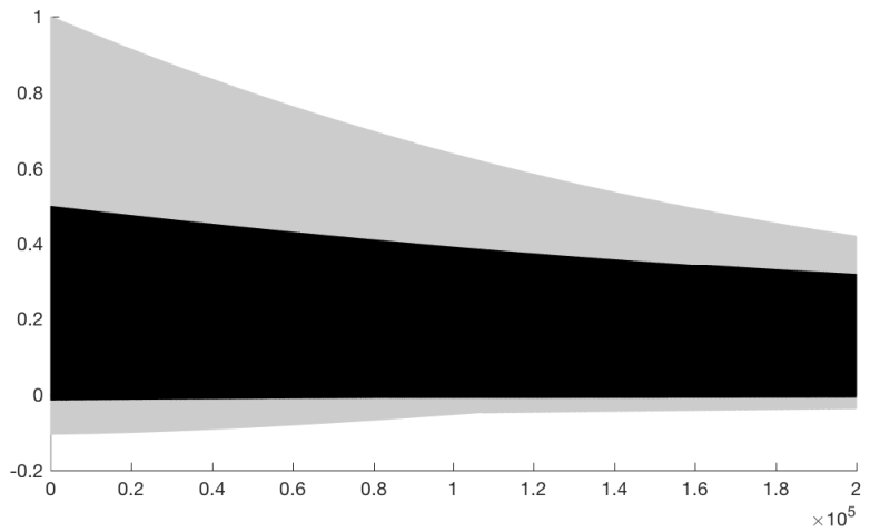
Finally, the sequence is not pre-uniformly wise because, when $k=k(n)=L-1=\log_{2}(n+1)-1$ , we estimate

\lim_{n\to\infty}\frac{1}{n}\sum_{i=1}^{n}(P^{[n]})^{k(n)}_{iv_{1}^{(1)}}\geq\lim_{n\to\infty}\frac{1}{n}2^{k(n)}=\lim_{n\to\infty}\frac{n+1}{2n}=\frac{1}{2},

where the first inequality follows if one deletes the term relative to the self loop in the matrix $P^{[n]}$ and observes that, being all nodes but $v_{1}^{(1)}$ of out-degree $1$ , $\sum_{i\neq v_{1}^{(1)}}(P^{[n]})^{k(n)}_{iv_{1}^{(1)}}$ coincides with the number of paths of length $L-1$ from the $L$ -th layer to $v_{1}^{(1)}$ .

Figure 8 illustrates the behavior of the dynamics in the very first steps proving that it is not pre-uniformly wise but that the average opinion slowly converges. Because of the computational complexity of the simulations (due to the large number of nodes), we are unable to clearly illustrate the asymptotic value on this graph for large number of layers $L$ or times $k$ . $\square$

These four examples complete the list of counterexamples in Lemma 7. We may make one obvious additional statement: finite-time wisdom implies one-time wisdom. The converse is not true, as established by the following counterexample.

Example 5 (The weighted double-star graph is one-time wise, but not two-time wise).

We define a sequence of weighted-neighbor matrices (recall Definition 1) as follows. For each $n$ , as illustrated in Figure 9, the graph is a double star with one root node (labeled $j$ ), $\sqrt{n}$ intermediate nodes (a representative node is labeled $h$ ) and $n$ leafs (a representative node is labeled $i$ ). For simplicity we assume $\sqrt{n}$ is a natural number. The symmetric edge weights are selected as follows: $1$ between root and the intermediate nodes and $1/\sqrt{n}$ between the intermediate nodes and the leafs. Note that the total number of nodes is $n+\sqrt{n}+1\asymp n$ . We add a self-loop with unit weight at the root node $j$ so that each matrix in the sequence is primitive.

Figure 9: A weighted double-star graph; we select

\alpha_{n}=1/\sqrt{n}

With these definitions, we have $W_{hj}=W_{jh}=1$ and, therefore, the weighted degree of the root note $j$ is $d_{j}=\sqrt{n}+1$ . We also have $W_{ih}=W_{hi}=\alpha_{n}=1/\sqrt{n}$ and, therefore, the weighted degree of each intermediate node $h$ is $d_{h}=1+\sqrt{n}\alpha_{n}=2$ and the weighted degree of each leaf $i$ is $d_{i}=\alpha_{n}=1/\sqrt{n}$ .

From the equality $P=\diag(W\mathbbold{1}_{n})^{-1}W$ defining a weighted-neighbor model, we compute $P_{ih}=d_{i}^{-1}W_{ih}=1$ , and $P_{jh}=1/(\sqrt{n}+1)$ so that the column sum of $P$ corresponding to an intermediate node $h$ is $\sqrt{n}\times 1+1\times 1/(\sqrt{n}+1)\asymp\sqrt{n}$ . Similarly, we compute $P_{hj}=d_{h}^{-1}W_{hj}=1/2$ so that the column sum of $P$ corresponding to the root node $j$ is $\sqrt{n}/2+1/(\sqrt{n}+1)$ . Therefore, the sequence is one-time wise.

Finally, for each leaf $i$ , we have $(P^{2})_{ij}=P_{ih}P_{hj}=1/2$ . Since there are $n$ leafs, the column sum of $P^{2}$ corresponding to the root node $j$ is at least $n/2\asymp n$ . The matrix sequence is therefore not wise at time two.

The presence of one-time wisdom and the lack of two-time wisdom is illustrated in Figure 10. $\square$

Figure 10: Weighted double star graph with

\sqrt{n}=10

and therefore

n=111

nodes. The time horizon is

T=100

. Individual opinions are in gray, the average opinion is in black. As proved in Example 5, the two figures illustrate that the graph is one time wise (see upper right corner figure) but not two time wise (nor wise). Specifically, the theoretical analysis shows that the the error at time 1 is of order

1/\sqrt{n}

and at time 2 of order

1

; indeed the black line illustrates an error magnitude that is much less than

1/10

at time 1 but not at time 2.

4 A sufficient condition for finite-time wisdom in general sequences of stochastic matrices

In this section we provide an insightful sufficient condition guaranteeing finite-time-wisdom for general sequences of matrices. The main proof idea is to introduce a recursive bound on the total influence of families of nodes. This bound amounts to a stronger property than finite-time wisdom and, unlike what occurs for finite-time wisdom, can be easily checked in terms of the matrix sequence.

We start with the following useful definition.

Definition 8 (Prominent families).

Given a sequence of stochastic matrices of increasing dimensions $\{P^{[n]}\in\mathbb{R}^{n\times{n}}\}_{n\in\mathbb{N}}$ , a sequence of sets of nodes $\{\mathcal{B}^{[n]}\subset\{1,\dots,n\}\}_{n\in\mathbb{N}}$ is said to be a $P^{[n]}$ -prominent family if

(i)

its size is negligible, that is, $|\mathcal{B}^{[n]}|=o(n)$ , but
(ii)

its total one-time influence is order $1$ , that is

$\frac{1}{n}\sum_{i=1}^{n}\sum_{j\in\mathcal{B}^{[n]}}P^{[n]}_{ij}\asymp 1.$

While one-time wisdom does not imply finite-time wisdom in general sequences (see Example 5), the following key result shows how the absence of prominent families is inherited by the powers of $P^{[n]}$ .

Theorem 9 (The absence of prominent families is persistent and implies finite-time wisdom).

Consider a sequence of stochastic matrices of increasing dimensions $\{P^{[n]}\in\mathbb{R}^{n\times{n}}\}_{n\in\mathbb{N}}$ . If there is no $P^{[n]}$ -prominent family, then

(i)

for every $k$ , there is no $(P^{[n]})^{k}$ -prominent family, and
(ii)

$P^{[n]}$ is finite-time wise.

In order to prove Theorem 9 we provide some general notions and then establish the recursive influence bound. Given an $n\times n$ stochastic matrix $P$ , define the maximum one-time influence of a set of nodes $\Phi_{P}:\{0,\dots,n\}\rightarrow\mathbb{R}_{\geq 0}$ by

\begin{cases}\Phi_{P}(0)=0,\\ \displaystyle\Phi_{P}(s)=\max\limits_{\mathcal{B}\subseteq\{1,\dots,n\},|\mathcal{B}|=s}\sum\limits_{i=1}^{n}\sum\limits_{j\in\mathcal{B}}P_{ij},\quad&s\in\{1,\dots,n\}.\end{cases}

Clearly, $\Phi_{P}(s)$ is non-decreasing in $s$ . Notice moreover that

\begin{split}\Phi_{P}(1)&=\max\limits_{i\in\{1,\dots,n\}}\sum\limits_{i=1}^{n}P_{ij}=\|P\|_{1},\\ \Phi_{P}(n)&=\sum_{i=1}^{n}\sum\limits_{j=1}^{n}P_{ij}=n.\end{split}

We can extend the definition of $\Phi_{P}$ and define $\Phi_{P}:\mathbb{R}_{\geq 0}\rightarrow\mathbb{R}_{\geq 0}$ by $\Phi_{P}(x)=\Phi_{P}(\lfloor x\rfloor).$ Note that $\Phi_{P}$ remains a non-decreasing function.

The following two statements are a straightforward consequence of the definition of the function $\Phi_{P}$ .

Remark 10.

(i)

The absence of $P^{[n]}$ -prominent families is equivalent to the following fact:

\displaystyle\text{for all }\{a_{n}\in\mathbb{R}_{\geq 0}\}_{n\in\mathbb{N}}\text{ satisfying }a_{n}=o(n),\Phi_{P^{[n]}}(a_{n})=o(n).

(18)

(ii)

Since $n^{-1}\|P^{[n]}\|_{1}=n^{-1}\Phi_{P^{[n]}}(1)$ , the previous statement and Theorem 3 together imply that, if there is no $P^{[n]}$ -prominent family, then $P^{[n]}$ is one-time wise. $\square$

The following technical result will play a crucial role in our derivations.

Lemma 11 (Recursive influence bound).

Let $P,Q$ be $n\times n$ stochastic matrices. For every $\delta>0$ and $s\in\{0,\dots,n\}$ , it holds

\Phi_{PQ}(s)\leq\Phi_{P}\left(\delta\Phi_{Q}(s)\right)+\frac{n}{\delta}.

Proof.

Define the shorthand $\mathcal{V}=\{1,\dots,n\}$ . Consider any $\mathcal{B}\subseteq\mathcal{V}$ and define

N_{\mathcal{B}}^{Q}(\delta)=\big\{h\in\mathcal{V}\;\big|\;\sum\nolimits_{j\in\mathcal{B}}Q_{hj}\geq\delta^{-1}\big\}.

Notice that

$\displaystyle\sum_{i\in\mathcal{V}}\sum_{j\in\mathcal{B}}(PQ)_{ij}$	$\displaystyle=\sum_{i\in\mathcal{V}}\sum_{h\in\mathcal{V}}\sum_{j\in\mathcal{B}}P_{ih}Q_{hj}$	(19)
	$\displaystyle=\sum_{i\in\mathcal{V}}\sum_{h\in N_{\mathcal{B}}^{Q}(\delta)}P_{ih}\sum_{j\in\mathcal{B}}Q_{hj}+\sum_{i\in\mathcal{V}}\sum_{h\notin N_{\mathcal{B}}^{Q}(\delta)}P_{ih}\sum_{j\in\mathcal{B}}Q_{hj}$
	$\displaystyle\leq\sum_{i\in\mathcal{V}}\sum_{h\in N_{\mathcal{B}}^{Q}(\delta)}P_{ih}+\sum_{i\in\mathcal{V}}\sum_{h\notin N_{\mathcal{B}}^{Q}(\delta)}P_{ih}\delta^{-1}$
	$\displaystyle\leq\Phi_{P}\left(\|N_{\mathcal{B}}^{Q}(\delta)\|\right)+\frac{n}{\delta},$

where last inequality follows from the definition of $\Phi_{P}$ and the trivial bound $\sum_{i\in\mathcal{V}}\sum_{h\notin N_{\mathcal{B}}^{Q}(\delta)}P_{ih}\leq 1$ . Note that

\Phi_{Q}(|\mathcal{B}|)\geq\sum_{h\in\mathcal{V}}\sum_{j\in\mathcal{B}}Q_{hj}\geq\sum_{h\in N_{\mathcal{B}}^{Q}(\delta)}\sum_{j\in\mathcal{B}}Q_{hj}\geq|N_{\mathcal{B}}^{Q}(\delta)|\cdot\delta^{-1},

which implies

|N_{\mathcal{B}}^{Q}(\delta)|\leq\delta\Phi_{Q}(|\mathcal{B}|).

Therefore,

\sum_{i\in\mathcal{V}}\sum_{j\in\mathcal{B}}(PQ)_{ij}\leq\Phi_{P}\left(\delta\Phi_{Q}(|\mathcal{B}|)\right)+\frac{n}{\delta}.

Now, fix a size $s$ and the proof is complete by computing the maximum value of the left and right-hand side over all subsets $\mathcal{B}\subseteq\mathcal{V}$ with $|\mathcal{B}|=s$ .

We are finally ready to prove the main result in this section.

Proof of Theorem 9.

We start by proving statement (i). Given Remark 10 (i), it suffices to to show that

\text{for all }\{a_{n}\in\mathbb{R}_{\geq 0}\}_{n\in\mathbb{N}}\text{ satisfying }a_{n}=o(n),\kern 5.0pt\Phi_{(P^{[n]})^{k}}(a_{n})=o(n).

(20)

We proceed by induction on $k$ . Indeed we know from our assumption that the statement in equation (20) is true for $k=1$ . We now suppose it is true for $k$ and we prove it for $k+1$ . We fix a sequence $\{a_{n}\}$ such that $a_{n}=o(n)$ . Lemma 11 implies

\Phi_{(P^{[n]})^{k+1}}(a_{n})\leq\Phi_{P^{[n]}}\left(\delta\Phi_{(P^{[n]})^{k}}(a_{n})\right)+\frac{n}{\delta}.

The induction assumption implies that $\Phi_{(P^{[n]})^{k}}(a_{n})=o(n)$ and, by Remark 10 (i), we have that

\Phi_{P^{[n]}}\left(\delta\Phi_{(P^{[n]})^{k}}(a_{n})\right)=o(n).

Therefore

\limsup_{n\to\infty}\frac{\Phi_{(P^{[n]})^{k+1})}(a_{n})}{n}\leq\frac{1}{\delta}

and, because $\delta$ is arbitrary,

\limsup_{n\to\infty}\frac{\Phi_{(P^{[n]})^{k+1})}(a_{n})}{n}=0.

This equality completes the proof by induction and proves statement (i). Statement (ii) follow from statement (i) considering that

\frac{1}{n}\|(P^{[n]})^{k}\|_{1}=\frac{1}{n}\Phi_{(P^{[n]})^{k}}(1).

5 A necessary and sufficient condition for pre-uniform wisdom in sequences of equal-neighbor matrices

In this section we focus on sequence of equal-neighbor stochastic matrices (recall Definition 1). For this setting we are able to provide a complete characterization of one-time, finite-time and pre-uniform wisdom. We start with a revised notion of prominence.

Definition 12 (Prominent individuals).

Given a sequence of stochastic matrices of increasing dimensions $\{P^{[n]}\in\mathbb{R}^{n\times{n}}\}_{n\in\mathbb{N}}$ , a sequence of individuals $\{k^{[n]}\in\{1,\dots,n\}\}_{n\in\mathbb{N}}$ is said to be $P^{[n]}$ -prominent if its total one-time influence is order $1$ , that is

\frac{1}{n}\sum_{i=1}^{n}P^{[n]}_{ik^{[n]}}\asymp 1.

In other words, a prominent individual is a prominent family composed of a single individual at each $n$ .

Remark 13.

Some comments are in order.

(i)

The absence of prominent families implies the absence of prominent individuals; but that the absence of prominent individual does not imply the absence of prominent family (e.g., take $\sqrt{n}$ nodes each with $\sqrt{n}$ neighbors with degree $1$ in an equal neighbor sequence).
(ii)

The existence of prominent individuals means that there exists a sequence of nodes $\{k^{[n]}\in\{1,\dots,n\}\}_{n\in\mathbb{N}}$ such that node $k^{[n]}$ possesses order $n$ neighbors with order $1$ degree. $\square$

We next show how the absence of prominent individuals and the notion of one-time wisdom play a key role in equal-neighbor sequences.

Theorem 14 (The absence of prominent individuals is necessary and sufficient for pre-uniform wisdom in equal-neighbor sequences).

Consider a sequence of equal-neighbor matrices of increasing dimensions $\{P^{[n]}\}_{n\in\mathbb{N}}$ . The following statements are equivalent:

(i)

there is no $P^{[n]}$ -prominent individual,
(ii)

the sequence is one-time wise, and
(iii)

the sequence is pre-uniformly wise.

In other words, one-time wisdom implies finite-time wisdom and pre-uniform wisdom for the setting of equal-neighbor sequences as well as wisdom for the setting of primitive equal-neighbor sequences. Recall that for more general sequences, e.g., the setting of weighted-neighbor models, one-time wisdom does not imply two-time wisdom (see Example 5).

Based on Theorem 14 (and specifically on the fact that one-time wisdom implies wisdom) and Example 2 (showing an example of a wise but not one-time wise sequence), we classify the equal-neighbor sequences as shown in Figure 11.

Figure 11: Logical relations among sets of equal-neighbor sequences with varying degree of wisdom. For each set we provide an example of a equal-neighbor sequence.

In order to prove Theorem 14 we establish some useful bounds.

Lemma 15 (One-norm bounds).

Any equal-neighbor matrix $P\in\mathbb{R}^{n\times{n}}$ satisfies, for all $k\in\mathbb{N}$ ,

\displaystyle\big\|\tfrac{1}{n}P^{k}\big\|_{1}

\displaystyle\leq 2\big\|\tfrac{1}{n}P\big\|_{1}^{1/2}.

(21)

Remark 16.

The square root is unavoidable, i.e., it is not possible to obtain a bound similar to (21) for equal-neighbor matrices that does not involve the square root of the one-norm of $P$ . For example, the double-star with $\sqrt{n}$ aperture is an example where $\|\tfrac{1}{n}P\|_{1}=1/n$ and $\|\tfrac{1}{n}P^{2}\|_{1}=1/\sqrt{n}$ . $\square$

Proof of Lemma 15.

Let $P=\diag(W\mathbbold{1}_{n})^{-1}W$ for a binary and symmetric $W$ , let $G$ denote the undirected graph defined by $W$ , pick a node $j\in\{1,\dots,n\}$ and a constant $\delta>0$ . Define

N_{j}(\delta)=\Big\{h\in\{1,\dots,n\}\;\Big|\;P_{hj}\geq\frac{1}{\delta}\Big\}=\{h\in N_{j}\;|\;d_{h}\leq\delta\}.

(22)

We now compute

	$\displaystyle P^{k}_{ij}$	$\displaystyle=\sum_{h=1}^{n}P^{k-1}_{ih}P_{hj}=\sum_{h\in N_{j}(\delta)}P^{k-1}_{ih}P_{hj}+\sum_{h\notin N_{j}(\delta)}P^{k-1}_{ih}P_{hj}$
		$\displaystyle\leq\sum_{h\in N_{j}(\delta)}P^{k-1}_{ih}P_{hj}+\sum_{h\notin N_{j}(\delta)}P^{k-1}_{ih}\frac{1}{\delta}$
		$\displaystyle=\sum_{h\in N_{j}(\delta)}P^{k-1}_{ih}P_{hj}+\frac{1}{\delta}.$

We now introduce the shorthand $\gamma_{j}^{(k)}=\sum_{i=1}^{n}P^{k}_{ij}$ for the $j$ -th column sum of $P^{k}$ and obtain

\displaystyle\gamma_{j}^{(k)}=\sum_{i=1}^{n}P^{k}_{ij}

\displaystyle\leq\sum_{i=1}^{n}\sum_{h\in N_{j}(\delta)}P^{k-1}_{ih}P_{hj}+\frac{n}{\delta}.

(23)

We change the order of summation and compute, for any $h\in N_{j}(\delta)$ ,

	$\displaystyle\sum_{i=1}^{n}P^{k-1}_{ih}$	$\displaystyle=\sum_{i=1}^{n}\sum_{\ell_{1}=1}^{n}\cdots\sum_{\ell_{k-2}=1}^{n}(d_{i}^{-1}W_{i\ell_{1}})(d_{\ell_{1}}^{-1}W_{\ell_{1}\ell_{2}})\cdots(d_{\ell_{k-2}}^{-1}W_{\ell_{k-2}h})$
		$\displaystyle=\sum_{i=1}^{n}\sum_{\ell_{1}=1}^{n}\cdots\sum_{\ell_{k-2}=1}^{n}d_{i}^{-1}(W_{\ell_{1}i}d_{\ell_{1}}^{-1})(W_{\ell_{2}\ell_{1}}d_{\ell_{2}}^{-1})\cdots(W_{\ell_{k-2}\ell_{k-3}}d_{\ell_{k-2}}^{-1})W_{h\ell_{k-2}},$

where we use the symmetry of $W$ , and reorganize the products inside the summation. We now upper bound $d_{i}^{-1}$ with $1$ , note that $\sum_{i=1}^{n}W_{\ell i}d_{\ell}^{-1}=1$ , and change the order of summation so that

	$\displaystyle\sum_{i=1}^{n}P^{k-1}_{ih}$	$\displaystyle\leq\sum_{\ell_{k-2}=1}^{n}\cdots\sum_{\ell_{1}=1}^{n}\sum_{i=1}^{n}(W_{\ell_{1}i}d_{\ell_{1}}^{-1})(W_{\ell_{2}\ell_{1}}d_{\ell_{2}}^{-1})\cdots(W_{\ell_{k-2}\ell_{k-3}}d_{\ell_{k-2}}^{-1})W_{h\ell_{k-2}}$
		$\displaystyle=\sum_{\ell_{k-2}=1}^{n}W_{h\ell_{k-2}}=d_{h}.$

We plug this inequality into (23) and adopt some additional bounds to obtain

\displaystyle\gamma_{j}^{(k)}

\displaystyle\leq\sum_{h\in N_{j}(\delta)}d_{h}P_{hj}+\frac{n}{\delta}\leq\Big(\max_{h\in N_{j}(\delta)}d_{h}\Big)\gamma_{j}^{(1)}+\frac{n}{\delta}.

Because $W$ is binary, we know that $h\in N_{j}(\delta)$ implies $d_{h}\leq\delta$ (see also definition (22)). The last inequality becomes:

\displaystyle\frac{1}{n}\gamma_{j}^{(k)}

\displaystyle\leq\delta\frac{1}{n}\gamma_{j}^{(1)}+\frac{1}{\delta}.

By selecting $\delta=\Big(\frac{1}{n}\gamma_{j}^{(1)}\Big)^{1/2}$ , we obtain that each column average of the $P^{k}$ satisfies

\displaystyle\frac{1}{n}\gamma_{j}^{(k)}

\displaystyle\leq 2\Big(\frac{1}{n}\gamma_{j}^{(1)}\Big)^{1/2}.

This inequality immediately implies inequality (21) in the theorem statement.

We are now ready to prove the main result of this section.

Proof of Theorem 14.

We start by showing the equivalence (ii) $\iff$ (iii). The fact that one-time wisdom (statement (ii)) implies pre-uniform wisdom (statement (iii)) for equal-neighbor sequences is a direct consequence of inequality (21) in Lemma 15. The converse implication (iii) $\implies$ (ii) is trivially true and stated in Lemma 7.

Next, we show the equivalence between the absence of prominent individuals (statement (i)) and one-time wisdom (statement (ii)). To do so, we prove the equivalence between the existence of prominent individuals and the lack of one-time wisdom. First, assume there exists a prominent individual, that is, as mentioned in Remark 13, a sequence of nodes $\{k^{[n]}\in\{1,\dots,n\}\}_{n\in\mathbb{N}}$ such that node $k^{[n]}$ possesses order $n$ neighbors in $G^{[n]}$ with order $1$ degree. In other words there exists a constant $\delta>0$ such that, recalling the definition in equation (22), we have $|N_{k^{[n]}}(\delta)|$ is of order $n$ . Then, from the equality (4),

	$\displaystyle\frac{1}{n}\\|P^{[n]}\\|_{1}$	$\displaystyle=\frac{1}{n}\max_{j\in\{1,\dots,n\}}\sum_{i=1}^{n}P^{[n]}_{ij}\geq\frac{1}{n}\sum_{i=1}^{n}P^{[n]}_{ik^{[n]}}$
		$\displaystyle=\frac{1}{n}\sum_{i\in N_{k^{[n]}}}d_{i}^{-1}W^{[n]}_{ik^{[n]}}\geq\frac{1}{n\delta}\sum_{i\in N_{k^{[n]}}(\delta)}W^{[n]}_{ik^{[n]}}$
		$\displaystyle=\frac{1}{n\delta}\|N_{k^{[n]}}(\delta)\|.$

This inequality shows that $\lim_{n\to\infty}\|\frac{1}{n}P^{[n]}\|_{1}$ cannot vanish and, therefore, the sequence of equal-neighbor matrices fails to be one-time wise.

Second, assume the sequence of equal-neighbor matrices fails to be one-time wise. Then there exist a constant $\alpha>0$ and a time $N$ such that, for all $n>N$ ,

\frac{1}{n}\max_{j\in\{1,\dots,n\}}\sum_{i=1}^{n}P^{[n]}_{ij}\geq\alpha.

In other words, there must exist a sequence of indices $\{k^{[n]}\in\{1,\dots,n\}\}_{n\in\mathbb{N}}$ such that $\sum_{i\in N_{k^{[n]}}}d_{i}^{-1}W^{[n]}_{ik^{[n]}}>\alpha n$ . Because each degree is lower bounded by $1$ , this inequality implies the existence of a prominent individual.

Remark 17 (Wisdom estimates for large by finite populations).

Lemma 15 leads to an explicit estimation of the rate at which finite time wisdom is achieved, namely the rate of convergence of $\ave(x^{[n]}(k)))$ to $\mu$ . Indeed, from the proof of Theorem 3 (equality (9) and the following steps) and inequality (21), we can estimate

\Var[\ave(x^{[n]}(k))]\leq\sigma^{2}\big\|\tfrac{1}{n}(P^{[n]})^{k}\big\|_{1}\leq 2\sigma^{2}\big\|\tfrac{1}{n}P^{[n]}\big\|_{1}^{1/2}.

Similar considerations can also be applied to the concept of uniform wisdom, working directly this time with the deviation probability. From the proof of Theorem 6 and applying again inequality (21), we obtain

\Prob\left[\sup\limits_{k\in\mathbb{N}}|\ave(x^{[n]}(k)))-\mu|\geq\delta\right]\leq\frac{18e\sigma^{2}}{\delta^{2}}\big\|\tfrac{1}{n}P^{[n]}\big\|_{1}^{1/2}\tau_{\textup{mix}}(P^{[n]}).

These bounds allow us to quantify how close to wisdom (finite or uniform) is a large but finite group of individuals whose opinions evolve according to an equal neighbor French-DeGroot model. They are particularly effective in those cases when the quantities $\big\|P^{[n]}\big\|_{1}$ and $\tau_{\textup{mix}}(P^{[n]})$ can be estimated, as it is the case for the Erdös-Rényi graphs and the preferential attachment model studied in Subsection 5.1.

5.1 The equal-neighbor model over prototypical random graphs

For equal-neighbor models, a sufficient condition to guarantee one-time and pre-uniformly wisdom is:

\frac{d_{\textup{max}}(n)}{d_{\textup{min}}(n)}=o(n),

(24)

where $d_{\textup{max}}(n)$ and $d_{\textup{min}}(n)$ denote, respectively, the maximum and minimum degree of the graph as a function of the network size $n$ . Indeed, let $k^{[n]}$ be a vertex of the graph and compute:

\displaystyle\frac{1}{n}\sum_{i=1}^{n}P^{[n]}_{ik^{[n]}}\leq\frac{1}{n}\sum_{i=1}^{n}\frac{1}{d_{\textup{min}}(n)}\leq\frac{1}{n}\frac{d_{\textup{max}}(n)}{d_{\textup{min}}(n)},

as $n\to\infty$ . If condition (24) holds, then $\frac{1}{n}\sum_{i=1}^{n}P^{[n]}_{ik^{[n]}}\to 0$ as $n\to\infty$ so that there exist no prominent individuals.

In this section we study the Erdös-Rényi and the Barabási-Albert preferential attachment models of random graph and we show that, using condition (24), they are both one-time wise with high probability. In contexts where we have a sequence of probability spaces labeled by parameter $n$ (in our case the number of nodes in the graph), the locution with high probability (w.h.p.) means with probability converging to $1$ as $n\to+\infty$ . In the case of a limit property, as the case of one-time wise, to assert that it holds w.h.p. means that, for every $\epsilon>0$ , $\Prob[\|\frac{1}{n}P^{[n]}\|_{1}<\epsilon]$ converges to $1$ for $n\to+\infty$ .

Example 6 (The equal-neighbor model over Erdös-Rényi graphs).

An Erdös-Rényi graph $G(n,p)$ is a graph with $n$ vertices and with each possible edge having, independently, probability $p$ of existing [10]. We focus on the case when $p={c\log(n)}/{n}$ with $c>1$ . In this regime $G(n,p)$ is known to be connected and aperiodic w.h.p.. Moreover, [9, Lemma 6.5.2] implies that there exists a constant $b>0$ such that $b\log n\leq d_{i}\leq 4c\log n$ for every node $i$ w.h.p.. This bound immediately implies that condition (24) holds w.h.p. and thus the Erdös-Rényi model is one-time wise (and pre-uniformly wise and wise) w.h.p.. Using the fact that [9] $\tau_{\textup{mix}}(P^{[n]})=O(\log(n))$ w.h.p., we now prove that this model is also uniformly wise. Indeed, w.h.p.

	$\displaystyle\big\\|\tfrac{1}{n}(P^{[n]})^{k}\big\\|_{1}\tau_{\textup{mix}}(P^{[n]})$	$\displaystyle\leq 2\big\\|\tfrac{1}{n}P^{[n]}\big\\|_{1}^{1/2}\tau_{\textup{mix}}(P^{[n]})$
		$\displaystyle=O\left(\frac{1}{n^{\frac{1}{2}}}\log n\right),\quad\text{as $n\to\infty$,}$

where the first inequality follow from equation (21). $\square$

We now present the preferential attachment model. Also in this case, it is possible to prove that the equal-neighbor models is one time wise and uniformly wise w.h.p..

Example 7 (The equal-neighbor model over preferential attachment graphs).

The Barabási-Albert preferential attachment model is a random graph generation model described as follows: vertices are added sequentially to the graph, new vertices are connected to a fixed number of earlier vertices, that are selected with probabilities proportional to their degrees. Specifically, assume a fixed number $m_{0}$ of initial vertices is given and, at every step, a new vertex is added and $m$ ( $m\leq m_{0}$ ) new edges are added, whereby the new vertex is connected to a prior node $i$ with a probability proportional to the degree $d_{i}$ of $i$ , that is $d_{i}/\sum_{j}d_{j}$ . After $t$ time steps, the model leads to a random graph with $t+m_{0}$ vertices and $mt$ edges. It is known [3, 5] that the degree distribution follows a power-law, that the minimum degree is $d_{\textup{min}}(n)=m$ (by construction), and that the maximum degree is of order $d_{\textup{max}}(n)\in\Theta(\sqrt{n})$ w.h.p..

The equal-neighbor Barabási-Albert model is one-time wise (and, therefore, also pre-uniformly wise and wise) w.h.p.. This follows again by checking condition (24):

\frac{1}{n}\frac{d_{\textup{max}}(n)}{d_{\textup{min}}(n)}=O\left(\frac{1}{n}\frac{\sqrt{n}}{m}\right)=O\left(\frac{1}{m\sqrt{n}}\right),\quad\text{as $n\to\infty$.}

Moreover, the equal-neighbor Barabási-Albert model is uniformly wise. Indeed, recall from [1] that the mixing time of the Barabási-Albert model is w.h.p. $\tau_{\textup{mix}}(P^{[n]})=O(\log(n))$ , so that w.h.p.

	$\displaystyle\big\\|\tfrac{1}{n}(P^{[n]})^{k}\big\\|_{1}\tau_{\textup{mix}}(P^{[n]})$	$\displaystyle\leq 2\big\\|\tfrac{1}{n}P^{[n]}\big\\|_{1}^{1/2}\tau_{\textup{mix}}(P^{[n]})$
		$\displaystyle=O\left(\frac{1}{n^{1/4}}\log n\right),\quad\text{as $n\to\infty$},$

where the first inequality follows from inequality (21).

Finally, we consider a super-linear preferential attachment model. Notice that the Barabási-Albert model is a linear preferential attachment in the sense that the probability of choosing a node in the network is linear in the degree of the nodes. If we consider a super-linear model with a probability of the form $\sim x^{p}$ with $p>1$ , then it is known [20] that there exists, w.h.p., a node with degree of order $n$ , while all other nodes have finite degrees. It follows that a sequence of prominent individuals exists in large populations and that, by Theorem 14, the super-linear preferential attachment model is neither wise nor finite-time wise. $\square$

6 Conclusions

This paper furthers the study of learning phenomena and influence systems in large populations. Our results provide an alternative and, arguably, a bit more realistic characterization of wise populations in terms of the absence of prominently influential individuals and groups. Future work includes extending these concepts to influence systems with time-varying and concept-dependent interpersonal weights and to other opinion dynamic models.

7 Acknowledgments

The first author thanks Dr. Noah E. Friedkin for an early inspiring discussion about naïve learning. This material is based upon work supported by, or in part by, the U.S. Army Research Laboratory and the U.S. Army Research Office under grant number W911NF-15-1-0577.

References

[1] D. Acemoglu, G. Como, F. Fagnani, and A. Ozdaglar. Opinion fluctuations and disagreement in social networks. Mathematics of Operation Research, 38(1):1–27, 2013. doi:10.1287/moor.1120.0570.
[2] D. Acemoglu, M. A. Dahleh, I. Lobel, and A. Ozdaglar. Bayesian learning in social networks. Review of Economic Studies, 78(4):1201–1236, 2011. doi:10.1093/restud/rdr004.
[3] A.-L. Barabási and R. Albert. Emergence of scaling in random networks. Science, 286(5439):509–512, 1999. doi:10.1126/science.286.5439.509.
[4] J. Becker, D. Brackbill, and D. Centola. Network dynamics of social influence in the wisdom of crowds. Proceedings of the National Academy of Sciences, 114(26):E5070–E5076, 2017. doi:10.1073/pnas.1615978114.
[5] B. Bollobás, O. Riordan, J. Spencer, and G. Tusnády. The degree sequence of a scale-free random graph process. Random Structures & Algorithms, 18(3):279–290, 2001. doi:10.1002/rsa.1009.
[6] P. Bonacich. Factoring and weighting approaches to status scores and clique identification. Journal of Mathematical Sociology, 2(1):113–120, 1972. doi:10.1080/0022250X.1972.9989806.
[7] M. H. DeGroot. Reaching a consensus. Journal of the American Statistical Association, 69(345):118–121, 1974. doi:10.1080/01621459.1974.10480137.
[8] P. M. DeMarzo, D. Vayanos, and J. Zwiebel. Persuasion bias, social influence, and unidimensional opinions. Quarterly Journal of Economics, 118(3):909–968, 2003. doi:10.1162/00335530360698469.
[9] R. Durrett. Random Graph Dynamics. Cambridge University Press, 2006. doi:10.1017/CBO9780511546594.
[10] P. Erdös and A. Rényi. On the evolution of random graphs. Publication of the Mathematical Institute of the Hungarian Academy of Science, 5(1):17–60, 1960.
[11] J. R. P. French. A formal theory of social power. Psychological Review, 63(3):181–194, 1956. doi:10.1037/h0046123.
[12] N. E. Friedkin. Theoretical foundations for centrality measures. American Journal of Sociology, 96(6):1478–1504, 1991. doi:10.1086/229694.
[13] N. E. Friedkin and E. C. Johnsen. Social Influence Network Theory: A Sociological Examination of Small Group Dynamics. Cambridge University Press, 2011.
[14] F. Galton. Vox populi. Nature, 75:450–451, 1907. doi:10.1038/075450a0.
[15] B. Golub and M. O. Jackson. Naïve learning in social networks and the wisdom of crowds. American Economic Journal: Microeconomics, 2(1):112–149, 2010. doi:10.1257/mic.2.1.112.
[16] M. O. Jackson. Social and Economic Networks. Princeton University Press, 2010.
[17] A. Jadbabaie, A. Sandroni, and A. Tahbaz-Salehi. Non-Bayesian social learning. Games and Economic Behavior, 76(1):210–225, 2012. doi:10.1016/j.geb.2012.06.001.
[18] D. A. Levin, Y. Peres, and E. L. Wilmer. Markov Chains and Mixing Times. American Mathematical Society, 2009.
[19] J. Lorenz, H. Rauhut, F. Schweitzer, and D. Helbing. How social influence can undermine the wisdom of crowd effect. Proceedings of the National Academy of Sciences, 108(22):9020–9025, 2011. doi:10.1073/pnas.1008636108.
[20] R. Oliveira and J. Spencer. Connectivity transitions in networks with super-linear preferential attachment. Internet Mathematics, 2(2):121–163, 2005. doi:10.1080/15427951.2005.10129101.
[21] A. V. Proskurnikov and R. Tempo. A tutorial on modeling and analysis of dynamic social networks. Part I. Annual Reviews in Control, 43:65–79, 2017. doi:10.1016/j.arcontrol.2017.03.002.
[22] W. E. Pruitt. Summability of independent random variables. Journal of Mathematics and Mechanics, 15:769–776, 1966. doi:10.1512/iumj.1966.15.15052.
[23] J. Surowiecki. The Wisdom Of Crowds. Anchor, 2004.

$\displaystyle\Prob\!\Big[\sup\limits_{k\in\mathbb{N}}\|Y^{[n]}(k)-Y^{[n]}\|>\delta/2\Big]$	$\displaystyle\leq\frac{8}{\delta^{2}}\sup\limits_{k\in\mathbb{N}}\Big\\|\frac{1}{n}(P^{[n]})^{k}\Big\\|_{1}\sum_{k}\exp\left(-\left\lfloor\frac{k}{\tau_{\textup{mix}}(P^{[n]})}\right\rfloor\right)$
	$\displaystyle=\frac{8e}{\delta^{2}}\sup\limits_{k\in\mathbb{N}}\Big\\|\frac{1}{n}(P^{[n]})^{k}\Big\\|_{1}\frac{1}{1-\exp\left(-\frac{1}{\tau_{\textup{mix}}(P^{[n]})}\right)}$
	$\displaystyle\leq\frac{8e}{\delta^{2}}\sup\limits_{k\in\mathbb{N}}\Big\\|\frac{1}{n}(P^{[n]})^{k}\Big\\|_{1}\tau_{\textup{mix}}(P^{[n]}).$	(15)

$\displaystyle\Prob[\|Y^{[n]}\|>\delta/2]$	$\displaystyle\leq\frac{4}{\delta^{2}}\Var[Y^{[n]}]=\frac{4}{\delta^{2}}(\pi^{[n]})^{\top}(\pi^{[n]})$
	$\displaystyle\leq\frac{4}{\delta^{2}}\\|\pi^{[n]}\\|_{\infty}$
	$\displaystyle\leq\frac{4}{\delta^{2}}\sup\limits_{k\in\mathbb{N}}\Big\\|\frac{1}{n}(P^{[n]})^{k}\Big\\|_{1}.$	(16)

Finite-Time Influence Systems and the Wisdom Of Crowd EffectThanks: Submitted to the editors DATE.

Abstract

keywords

Funding.

1 Introduction

1.1 Review of notation and preliminary concepts

Definition 1 (Equal-neighbor, directed equal-neighbor, and weighted-neighbor matrices).

2 Wisdom in sequences of stochastic matrices: definitions and basic results

Definition 2 (Wisdom notions).

Theorem 3 (Necessary and sufficient conditions for finite-time wisdom and wisdom).

Proof.

Remark 4 (Estimation theory interpretation).

Definition 5 (Pre-uniform wisdom).

Theorem 6 (A sufficient condition for uniform wisdom).

Proof.

3 Basic implications and counterexamples

Lemma 7 (Basic implications and counterexamples).

Example 1 (The star graph is neither wise nor finite-time wise).

Example 2 (The union/contraction of star and complete graph is wise, but not one-time wise).

Example 3 (The path graph with biased weights is finite-time wise, but not wise).

Example 4 (The reversed binary tree with root-leaves edges is wise and finite-time wise, but not pre-uniformly wise).

Example 5 (The weighted double-star graph is one-time wise, but not two-time wise).

4 A sufficient condition for finite-time wisdom in general sequences of stochastic matrices

Definition 8 (Prominent families).

Theorem 9 (The absence of prominent families is persistent and implies finite-time wisdom).

Remark 10.

Lemma 11 (Recursive influence bound).

Proof.

Proof of Theorem 9.

5 A necessary and sufficient condition for pre-uniform wisdom in sequences of equal-neighbor matrices

Definition 12 (Prominent individuals).

Remark 13.

Theorem 14 (The absence of prominent individuals is necessary and sufficient for pre-uniform wisdom in equal-neighbor sequences).

Lemma 15 (One-norm bounds).

Remark 16.

Proof of Lemma 15.

Proof of Theorem 14.

Remark 17 (Wisdom estimates for large by finite populations).

5.1 The equal-neighbor model over prototypical random graphs

Example 6 (The equal-neighbor model over Erdös-Rényi graphs).

Example 7 (The equal-neighbor model over preferential attachment graphs).

6 Conclusions

7 Acknowledgments

References

Finite-Time Influence Systems
and the Wisdom Of Crowd EffectThanks: Submitted to the editors DATE.