Estimating the Rate Constant
from Biosensor Data via
an Adaptive Variational Bayesian Approach
The means to obtain the rate constants of a chemical reaction is a fundamental open problem in both science and the industry. Traditional techniques for finding rate constants require either chemical modifications of the reactants or indirect measurements. The rate constant map method is a modern technique to study binding equilibrium and kinetics in chemical reactions. Finding a rate constant map from biosensor data is an ill-posed inverse problem that is usually solved by regularization. In this work, rather than finding a deterministic regularized rate constant map that does not provide uncertainty quantification of the solution, we develop an adaptive variational Bayesian approach to estimate the distribution of the rate constant map, from which some intrinsic properties of a chemical reaction can be explored, including information about rate constants. Our new approach is more realistic than the existing approaches used for biosensors and allows us to estimate the dynamics of the interactions, which are usually hidden in a deterministic approximate solution. We verify the performance of the new proposed method by numerical simulations, and compare it with the Markov chain Monte Carlo algorithm. The results illustrate that the variational method can reliably capture the posterior distribution in a computationally efficient way. Finally, the developed method is also tested on the real biosensor data (parathyroid hormone), where we provide two novel analysis tools – the thresholding contour map and the high order moment map – to estimate the number of interactions as well as their rate constants.
, , and
Chemnitz University of Technology, National University of Singapore and Karlstad University
1 Introduction
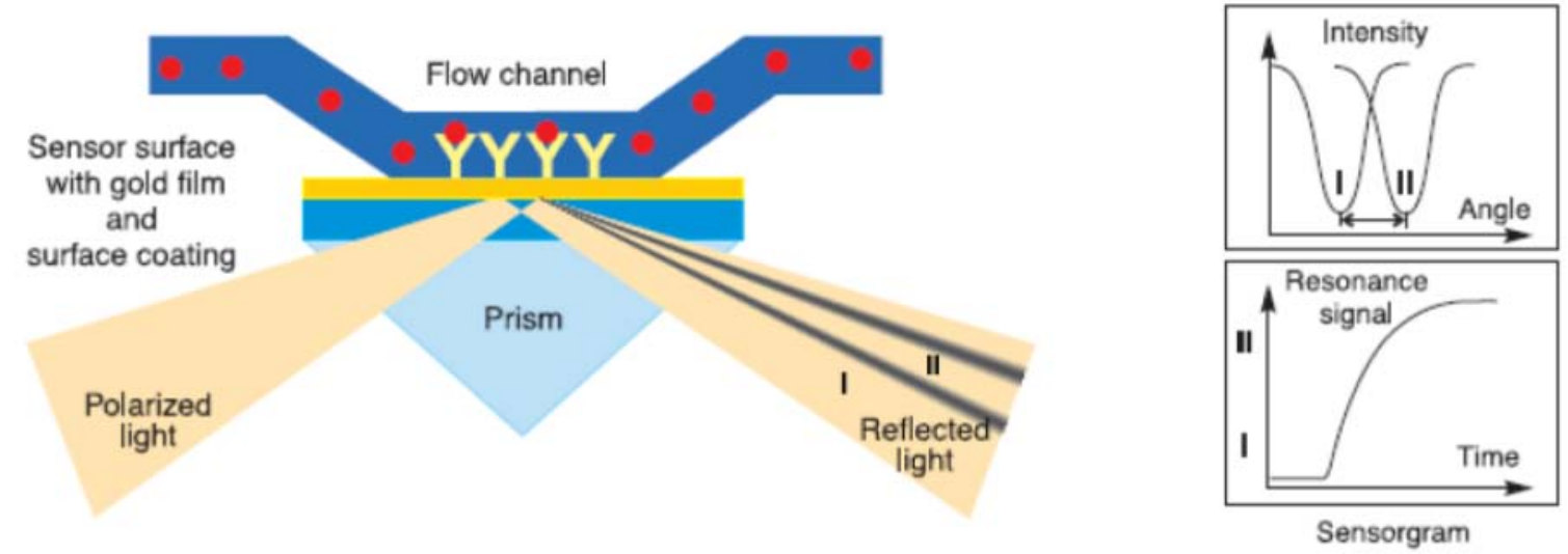
In the modern world, biosensors have made a significant impact in many fields, such as antibody-antigen interactions, immunology, virology, and the pharmaceutical industry (Sanvicens et al. 2011; Elmlund et al. 2015). Hence, during the last few decades, there has been an accelerated technological development of biosensor instruments, e.g., surface plasmon resonance, quartz crystal microbalance, etc. A simplified biosensor system is presented in Figure 1, and its physical mechanism is briefly discussed in Appendix A. To design an appropriate biosensor instrument that is biocompatible or specifically functionalized, scientists must know the physical chemistry of biomolecular/cell surface interactions (Telesca et al. 2012). The reliable analysis of biomolecular interactions is crucial in both science and the industry, e.g., it is required to fulfill modern drug quality assurance criteria. In order to understand the interactions, scientists collect biosensor data that measures the analyte biomolecules of several different concentrations on a sensor chip with immobilized ligand molecules that form complexes with analytes. This kind of biosensor data is usually called a sensorgram, where the systems response, proportional to total complex concentration, is measured over time for different analyte injections. In this paper, we focus on this particular type of data and aim to obtain information about the interactions, i.e., their numbers and the corresponding rate constants. The biosensor data is traditionally processed using a simple model fitting procedure assuming just one, or perhaps two, distinct interactions. These traditional approaches might not reflect the true, complicated, and heterogeneous molecular interactions for large active pharmaceutical ingredients, and can thus lead to wrong mechanistic conclusions. Therefore, a more advanced analysis of the biosensor data is necessary to avoid the costly and time consuming procedure of repeating the same ligand-analyte binding experiment over and over using chips with different ligand binding or different buffers, etc., until one of the tests results in “good enough” data that works with the standard rate constant estimation (Gray and Pierce 1985).
1.1 Existing work in Statistics and Computational Chemistry
The problem of estimating the chemical rate constants of interactions through statistical approaches has been investigated for long time (Box and Draper 1965; Atherton, Schainker and Ducot 1975; Ziegel and Gorman 1980; Komorowski et al. 2011; Gupta and Rawlings 2014; Pischel, Sundmacher and Flassig 2017). To our best knowledge, most of the existing statistical approaches require a priori knowledge of the number of interactions in a chemical reaction, i.e., they first assume the existence of parallel reaction (due to potential interactions), and then estimate the rate constants for corresponding interactions. Therefore, in practice, the problem is usually solved by a two-step strategy. The first step is to determine the number of interactions by dimensionality reduction technique (e.g., principal component analysis, regression tree (Loh and Zheng 2013)), and then fit the data to the parameters (i.e., rate constants correspond to these reactions). It is clear that the first step partially determines the quality of the results in the second step. However, it can be observed that the second step procedure also potentially has a positive influence on the estimation in the first step, particularly when the data is under-sampled and affected by large noise. Therefore, the separation of the procedure into two steps does not seem optimal. The question that now arises is whether the number of interactions and the values of rate constants corresponding to each interaction in a single step can be estimated from the biosensor data, therefore making the modeling more robust. These considerations form the motivations behind our work.
Another line of research, inspired by Adsorption Energy Distribution (AED) calculations (Stanley and Guiochon 1995), which are successfully used for steady-state data usually from small molecular systems, as well as a couple of numerical solvers for dynamic biosensor data, such as the Interaction Distribution (ID) (or Interaction Map) (Svitel et al. 2003; Altschuh et al. 2012) and Adaptive Interaction Distribution Algorithm (AIDA) (Zhang et al. 2018), have recently gained much attention. With these solvers, one can see the number of interactions in the system, along with their associated rate constants, as peaks on a surface. The mathematical basis behind these solvers is to use a single step model to estimate the number of rate constants and their values simultaneously. They utilize regularization methods to impose a sense of well-posedness for the model and solve the resulting deterministic problems by optimization. However, the result of these methods strongly depends on the choice of system parameters, e.g., the type of regularization penalty and the value of the regularization parameter. For our application, as well as other problems where no ground truth is available, the problem of selecting the regularization penalty term and the regularization parameter remains an open issue (Fan and Lv 2008), as most tuning parameters such as the generalized cross-validation (GCV) (Tibshirani 1996), style statistics (Efron et al. 2004), and the consistent estimator of degrees of freedom of the LASSO in the , AIC, and BIC criteria (Zou, Hastie and Tibshirani 2007), are based on an asymptotic property that is practically infeasible.
The shortage of existing methods motivates us to combine statistical and deterministic methods to develop a more robust single step approach via a statistical strategy. Note that this high level idea has been used in Gorshkova et al. 2008 to some extent. However, from a mathematical viewpoint, their method can still be classified in the branch of deterministic methods, since it estimates the distribution of rate constant directly by solving a special regularized optimization problem. Though the authors have taken into account the contribution of a prior expectation of rate constants on the regularization term in their optimization formulation, the mathematical model should be deterministic if one considers the distribution of rate constant, which is also termed as the rate constant map, as a deterministic object (i.e. an element in the space of functions). Furthermore, the justification of rate constants as random variables is missing, and no uncertainty quantification is discussed under their framework. Meanwhile, the difficulty of choosing an appropriate regularization parameter remains. This motivates us to regard the rate constant map as a random variable, which incorporates the regularization in a completely different way, and overcomes the difficulty of selecting regularization parameter, hence may carry the intrinsic information from the uncertainty quantification of the rate constant map.
1.2 Motivation
As discussed above, due to the diversity of data structure and the appearance of noise in many biosensor problems, the existing methods do not work efficiently. The central problem is that most of them are not capable of inferring the interaction information correctly. For instance, in the assumption that two interactions exist in our biosensor system, the exact value of rate constants in our data structure called the dissociation constant (measures the rate at which a molecule complex diassociates) and association constant (rate at which molecules form complexes), see Appendix A for details, are displayed in (a) of Figure 2. This means that two parallel interactions exist and their corresponding rate constants are and . Now, we solve the problem using the conventional rate constant map method, which will be introduced later in Section 2 and Appendix A. This method provides a map of distribution of rate constants (called a rate constant map), from which we can figure out the number of interactions and the rate constants of these interactions. The desired estimated rate constant map should exhibit the information of the interactions. One example of this rate constant map is displayed in (b) of Figure 2, where people can easily derive the interaction numbers and rate constants from the peaks of the rate constant map. However, in many cases, the regularized deterministic approaches cannot offer the rate constant map that is correctly shaped. For instance, in our parathyroid hormone application, the Tikhonov regularization provides an oversmoothing effect on the rate constant map, while, the sparse regularization offers a rather unsatisfactory reconstruction of the rate constant map, see Figure 3 for details. This motivates us to build new statistical models and investigate the methods that can efficiently estimate the rate constant map with uncertainty quantification, from which we can explore the intrinsic heterogeneity of the biosensor system – the interaction information including the number of interactions and the corresponding rate constants. The philosophy of our approach is to assume that the rate constants are no longer static. By utilizing the non-static rate constants, where the rate constant map is modeled as a high dimensional random variable, we will be able to investigate the distribution of and provide estimates of the variability. Based on the estimated distribution of , we can produce different kinds of maps (e.g., (b) in Figure 2 or (a) and (b) in Figure 3) which provides a multi-scale perspective of the rate constant map. It turns out that the random rate constant map can be used to find the interaction information, e.g., the number of the interactions and rate constants for each interaction, which will be called the intrinsic quality of a chemical system.


In comparison with classical deterministic regularization methods, Bayesian approaches have distinct features for inverse problems (in our case, the inverse problem is the estimation of interaction information from indirectly measured biosensor data) that make them attractive for statistical inference (Bernardo and Smith 1994; Kennedy and ÓHagan 2001; Evans and Stark 2002; Kaipio and Somersalo 2007). First, the Bayesian posterior distribution provides uncertainty quantification by assigning probabilities to the space of all possible inverse solutions that are consistent with the observed data. This uncertainty quantification is lacking in all the deterministic regularization methods, which only yield one single solution as a point estimate. Second, the use of prior distribution allows more flexibility in modeling. For instance, sparsity-inducing priors such as the spike-and-slab prior can be used if sparse solutions are desirable for high dimensional models. Constraints on the parameter space, or the space of solutions in our context, can be imposed directly through constraining the support of the prior distribution. Third, the tuning parameters that are used in the frequentist regularization methods become hyper-parameters in the Bayesian framework. They are usually assigned some hyper-priors and can hence be made fully adaptive to the observed data. On the other hand, since the posterior distribution does not have an analytically tractable closed form in most cases, Bayesian inference typically requires the numerical sampling of the posterior distributions by Markov chain Monte Carlo (MCMC), which can be computationally intensive and may suffer from slow mixing due to high dimensionality or strong correlations between the parameters in their joint posterior distribution. As an alternative approach, the variational Bayesian (VB) inference (Bishop 2006; Blei, Kucukelbir and McAuliffe 2017) has gained popularity for its computational efficiency over posterior sampling methods in such complex Bayesian models. VB approximates the true posterior distribution with a family of computationally tractable distributions by minimizing the KL divergence between them. Although it has been empirically observed that VB occasionally underestimates the posterior variances, the gain in computational efficiency from VB is substantial in many applications; see, e.g., Parisi 1988, Peterson and Anderson 1987, Jordan et al. 1999, Wainwright and Jordan 2008, Jin and Zou 2010 and references therein.
In this paper, we build a Bayesian framework for uncertainty quantification in the biosensor problem and propose a new VB approach for computing the posterior distribution. Our VB approach is novel and motivated by three physical facts that are unique to the biosensor problem, as well as other similar problems, modeled by the integral equations (1). First, in our real world biosensor problem, the noise structure can be heterogeneous among different sensorgrams, which results in extremely high dimensionality of the parameter spaces that makes any posterior sampling algorithms such as the MCMC practically infeasible. Therefore, we develop a VB approach to circumvent the computational problem. Second, the solution of the rate constant map must be nonnegative for meaningful physical interpretation. This fact requires a constrained prior support and eventually a new VB algorithm that differs from the existing ones. Finally, the dimensionality of parameter space in most existing statistical models should be fixed, which requires the a priori knowledge of the distribution of rate constants in the biosensor system that is actually unknown before we estimate them. To overcome this difficulty, based on the newly developed VB algorithm we introduce an adaptive discretization technique that automatically adjusts the dimensionality of solution space during the evolution of our algorithm, according to the uncertainty quantification of the obtained temporary qualities.
1.3 Objective of the paper
In Section 2, based on the rate constant map theory, we establish a single step model connecting the biosensor data and the rate constant map, which is used for estimating the number of interactions and the rate constants simultaneously. Section 3 presents our newly developed method – an Adaptive Variational Bayesian Approach (AVBA) – for solving the proposed single step model. In Section 4, we illustrate the approach using an artificial problem, and compare its performance with the MCMC algorithm. The proposed method is tested on real biosensor data (parathyroid hormone) in Section 5, where we will develop two AVBA-based analysis tools that represent the intrinsic property of the interaction, and can be used for estimating the number of interactions as well as their rate constants. Finally, concluding remarks are given in Section 6.
2 A mathematical model for estimating the rate constant map
As mentioned before, in this work, we use the rate constant map (i.e., the distribution of association constant and dissociation constant ) to explore the interaction information, i.e., their numbers and (active) rate constants. Based on the Rate Constant Map Theory, see details in the Appendix A, the measured sensorgram , which is dependent on the analyte concentration and time , and the rate constant map are related through the following integral equation
| (1) |
where is the interested domain of rate constants, and the kernel function is defined as
| (2) |
where the physical meaning of parameters can be found in Appendix A. All of them are given constants.
Since the solution to the integral equation (1) does not have an analytically closed form, we have to solve (1) numerically. Moreover, in order to represent the rate constant map on computer, we need to discretize the function by a vector , associated with appropriate coordinates. By slightly abusing the notation, we shall call the rate constant map as well. In this work, we adapt the finite element technique for discretization. The relation between and its finite element approximation is provided in the supplementary material. We discretize our bounded domain by mesh using non-overlapping triangles with the standard shape regularity assumption. Introduce the finite element space of piecewise linear elements on the triangulation with the number of notes . Then, the projection of in (denote as ) can be decomposed as
| (3) |
where are the coordinates of under basis of the linear space .
Remark 1.
The dimensionality of approximate solution space cannot be fixed, since we have no a priori information about the distribution of peaks of the rate constant map , and cannot provide a good mesh which nodes hit or close to the positions of the peaks of . A naive way to capture the locations of the peaks of is to use an intensive grid with large so that every possible peak is located in a small neighborhood of a node of mesh. However, such an idea cannot be implemented in practice due to computational complexity. Alternatively, in this work, we start with a small paired with a coarse mesh , and then increase with a finer local mesh that only covers the region with possible peaks of until an approximate solution with satisfactory accuracy is obtained. Hence, instead of a fixed model (5) below, our algorithm will deal with a sequence of models of type (5) with dynamic dimensionality .
Furthermore, denote by the measured sensorgram with the injection and the time grid . Then, using the decomposition (3) and considering the inaccuracy of the measurement data, the finite element approximation of integral equation (1) can be written as a system of algebraic equations:
| (4) |
where , is the additive error for -th sensorgram, and matrix is defined by
Denote , and , where for column vectors and , . Then, the system (4) can be rewritten into a compact form
| (5) |
The deterministic approaches solve (5) by the iterative regularization (e.g., the Landweber method Engl, Hanke and Neubauer 1996), or the variational regularization with appropriate regularization term (e.g., the Tikhonov method), to obtain a regularized approximate solution of (5). Using the obtained , an approximate rate constant map can be reconstructed by (3), which is a function well defined in the whole domain . The active association and dissociation constants ( and ) for the given kinetic reaction process of the biomolecular system should be the peaks in the estimated rate constant map , see Svitel et al. 2003 and Altschuh et al. 2012. In this work, we refer to these peaks as the Intrinsic Property of the Interaction (IPoI). Now, the problem at hand is how to determine the IPoI in a chemical reaction through the single step model (1) (or its finite dimensional analogue (5)). This problem is seriously ill-posed since (i) one can always construct a large number of (deterministic) rate constant map satisfying the equation (1). In the reduced finite dimensional model (5), various numerical experiments have shown that . (ii) Note that the integral operator in (1) is a compact operator, which is affected by an instability phenomenon where a small amount of noise in the measurement data can lead to enormous errors in the estimates (Tikhonov and Arsenin 1977). Moreover, solutions to the deterministic models, e.g., the regularized solutions in Svitel et al. 2003, Altschuh et al. 2012, Gorshkova et al. 2008 and Zhang et al. 2018, do not represent the pure information of IPoI even though the experimental data is accurate enough. This phenomenon implies that the deterministic regularized solutions contain redundant information about a chemical reaction besides the IPoI. This drawback, as well as the problem of choosing a regularization term in the deterministic models aforementioned, motivates us to model the quantity in (5) (or in (1)) as a random vector (or function), from which we can study the uncertainty of the rate constant. As demonstrated in Section 5, the uncertainty of the quantity can be used to interpret the difference between the deterministic solution of (5) and the IPoI.
3 An adaptive variational Bayesian approach
3.1 Bayesian framework
A detailed understanding of the dynamics of the rate constant map given data and the model (5) is crucial in the context of our problem.
For simplicity, a Gaussian distribution of noise on each sensorgram is customarily assumed, i.e., () are independent and identically distributed (i.i.d.) additive Gaussian random vectors with mean zero and variance , where denotes the identity matrix of size . The assumption of normality is preferred due to the fact that Gaussian noise is present at the sensorgrams, and sensorgram noise is usually much smaller than the signal. Although correlated sensorgram noise is more realistic than “homogenerous” sensorgrams, this could complicate the problem. Then, the likelihood is given by
| (6) |
where denotes up to a multiplicative normalizing constant, and the covariance matrix of noise .
A natural mechanism for regularization is in the form of prior information. A versatile prior distribution of is the Markov random field prior; see Babacan, Molina and Katsaggelos 2008 for details. Define as the indicator function on the set , i.e. for , while for . Denote by the nonnegativity by components. For computational tractability, we use the following conjugate prior distribution
| (7) |
where the matrix encapsulates the structure of the interactions between neighboring components of the solution . is given and assumed to be full rank. Note that our choice of (7) also reflects the physical meaning of the rate constant. If the hyper-parameters, and , are given and the nonnegative constraint of the solution is ignored, the prior of in (7) for the maximum a posteriori estimate is exactly the same as the -type penalty term in the classical variational regularization theory (Stuart 2010), where denotes the standard Euclidean norm of a vector or the Frobenius norm of a matrix. For the classical Tikhonov regularization, stands for the discrete Laplacian.
To complete the model specification, we impose conjugate priors on the parameters and . In other words, for each of these parameters, we impose an independent inverse-gamma prior with the density , where is the shape parameter, is the scale parameter, and denotes the standard Gamma function. Then, plugging-in the density functions in (5), the posterior distribution of given the data is
| (8) |
where the values of hyperparameters and are given based on simulation results of artificial problems. The posterior distribution in (8) is the full Bayesian solution to our finite model (5), and it encapsulates all the information including IPoI. However, due to the high dimensionality of , (8) is also a distribution that lives in a space of very high dimension, e.g., , for our real data. Hence, it is advisable to develop tools for exploring this very high dimensional posterior distribution. In the next section, we develop an approximate inference method based on the mean field variational approximation for exploring the posterior in (8).
3.2 Variational approximation algorithm
Due to the presence of several variance parameters, the posterior distribution (8) does not have an explicit closed form. One way to explore this high dimensional posterior is to perform posterior sampling based on MCMC algorithms. Although the MCMC has the advantage of being asymptotically exact (Robert and Casella 2004), its convergence is also often known to be difficult to diagnose (Brooks et al. 2002; Bishop 2006), and it suffers from slow mixing in the presence of high dimensional parameters. As the dimensionality of the problem in the biosensor system is extremely large, we shall take an alternative route and focus on the variational approximation approach. The essential idea of variational methods consists of first transforming the problem into an equivalent optimization problem, and then obtaining an approximate distribution to the true posterior by solving the optimization problem inexactly. The idea behind VB approximation is to find a family of tractable distributions to approximate the posterior density by minimizing the Kullback-Leibler (KL) divergence (Kullback 1988), while still capturing distinct features of the posterior distribution (8) in a computationally efficient way.
The KL divergence is a non-symmetric measure of the difference between two probability distributions, and is defined as
| (9) |
where is a normalizing constant, and the global distribution has the form
| (10) |
Note that minimizing the KL distance in (9) is equivalent to minimizing the first term, which is termed as the evidence lower bound and denoted by ELBO (Blei, Kucukelbir and McAuliffe 2017). In this way, we have successfully transformed the sampling problem into an equivalent optimization problem of finding a simpler distribution by minimizing .
If we impose no constraint on the approximation , minimizing is numerically intractable. The intractability is largely due to the correlations among the parameters. To enable the computational tractability, we adapt the idea of mean-field variational family (Wand et al. 2011; Blei, Kucukelbir and McAuliffe 2017), and impose an independence condition among the parameter components and as
| (11) |
Under assumption (11), we can find an effective approximate posterior density, denoted by hereafter, using an alternating direction iterative algorithm, i.e., at -th step, we solve the following optimization problems:
| (12) |
Here and later on, the (superscript and subscript) index denotes the quantity of interest at -th iteration of the algorithm. Using condition (11), one can derive the explicit formulas for the minimizers of the optimization problems in (12) by examining the optimality system; i.e., the following theorem holds.
Theorem 1
Assume that the conditional independence condition (11) holds. Then, the minimizers of the optimization problems in Algorithm 1 at each iteration have the following explicit formulas:
| (13) |
where the density function for truncated normal distribution is
| (14) |
with and is the expectation with respect to the density .
In practice, the value of can be estimated numerically. The proof of Theorem 1 follows a standard argument in theory of variational inference, and we provide a sketch in the supplementary material (Zhang et al.).
Now, we discuss the convergence issue of scheme (12).
Theorem 2
The sequence generated by scheme (12) converges, upon a subsequence, to a stationary point of the KL distance functional , which satisfies
| (15) |
We refer readers to Appendix B for the proof of Theorem 2. To that end, let us consider the stopping principle of our scheme. Various stopping criteria exist for an iterative algorithm, e.g., ELBO is usually calculated (whenever possible) as a stopping criterion in the variational inference. For our problem, a natural and simple stopping criterion is to utilize the mean and covariance of the interested quantity – the rate constant map . Hence, we define the accuracy of our algorithm as
| (16) |
Finally, by coupling the stopping criteria and Theorem 1, we offer a variational Bayesian algorithm for reconstructing the rate constant map in the biosensor system in Algorithm 1.
3.3 An adaptive strategy to improve the quality of the rate constant map
As mentioned in Remark 1, we start with a low dimensionality of solution space where the rate constant map is only estimated on a set of coarse distributed points in . Therefore, the resolution of the rate constant map is quite low. In order to improve the quality of the estimated rate constant map , we adopt the idea of the oriented adaptive discretization, from numerical technique in finite element methods (Chen, Holst and Xu 2009; Zhang et al. 2018). The idea, combined with our approach, is to first solve the problem (1) through the variational Bayesian approach (Algorithm 1), obtaining the solution (the distribution of the random vector ) to the current triangulation. The quality is then estimated using the solution, and is used to mark a set of triangles to be refined. Triangles are refined in a way that maintains two of the most important properties of the triangulations: shape regularity and conformity.
Given an estimated distribution , let and be the sample mean, the lower and upper endpoints of the 95% confidence interval by samples from Algorithm 1. Define by the variation of the mean vector over the elements , i.e. . Similarly, we can define the variation of and , denoted by and respectively. Finally, define the refinement indicator by
| (17) |
Then, the refinement should be done in the triangles of all points in the finite element mesh where the function achieves its maximum; i.e., refine the mesh in such triangles of where
| (18) |
where are numbers which should be chosen computationally.
Finally, we use the longest edge refinement rule for dividing the marked triangles, so that the mesh obtained by this dividing rule still conforms and has a shape regular (Rivara 1984). Note that apart from the marked triangles, the additional triangles are also refined to recover the conformity of triangulations. In this work, we also control the number of elements added to ensure the overall optimality of the refinement procedure.
Let us present our main algorithm for solving the two-dimensional Fredholm integral equation of the type (1) in Algorithm 2.
4 Simulation study

This section presents the numerical results for the inverse problem (1), of which the adaptive variational Bayesian approach (AVBA), i.e., Algorithm 2, is used to illustrate its accuracy and flexibility. The simulation consists of three steps. First, a simulated response function is generated by computer according to (1) for a given rate constant map in the domain – see (a) in Figure 4. Denote by (see (b) in Figure 4) the collected exact data at a uniform time grid (, , and ), at a uniform analyte concentration grid ( and ). The synthetic noisy data is generated by
where indicates the noise level, and is a Gaussian random variable with zero mean and standard deviation . At the last step of the simulation, the observation data is processed through our algorithm, and the retrieved rate constant map is compared with the input map. To assess the accuracy of the approximate solution, we define the -norm relative error for an estimated random vector with distribution as
A demonstration of Algorithm 2 can be found in the supplementary material. The fundamental assumption of our approach, according to (11), is the conditional independence of random variables given the data . To examine the assumption (11), we compute the Pearson correlation coefficients , and between the vectors , and respectively, from the MCMC samples. The correlation coefficient between the vector and scalars are computed component-wise, i.e., with . The results, for the example in the supplementary material, are shown in Figure 5, where the abscissa (or ) denotes the th (or th) component. Overall, the correlation coefficients between and are very small, with a maximum norm , smaller than 0.004 for all three noise levels. The correlation coefficients between and are also small with a maximum norm smaller than 0.08 for all three noise levels. The correlation coefficients between and are slightly larger with the maximum norm close to 0.14. Hence, we can conclude that the correlation between , and is relatively weak.

Now, we investigate the robustness of Algorithm 2. We first study the sensitivity of the numerical results with respect to the prior parameters and , and illustrate the rationale behind these choices in the following examples. If the value of is not too large, the distributions of and in (15) are dominated by and in the numerators and , and can thus only have a marginal impact on the algorithm. Therefore, we only study the influence of parameters . Since plays the same role in the algorithm, we only present the result for here. The results are displayed in Table 1, where the data noise level equals 1%, and parameters (), and are all set as 1. The results show that both the estimated rate constant mean map and the conditional independence assumption (11) seem relatively independent of the parameters and for the magnitude of the relative error L2Err, and the correlation coefficients , and remain almost unchanged as the value of and varies.
| L2Err | |||||
| 0.0001 | 0.0001 | 0.0661 | 0.0032 | 0.0130 | 0.2247 |
| 0.01 | 0.01 | 0.0659 | 0.0002 | 0.0304 | 0.0414 |
| 1 | 1 | 0.0658 | 0.0029 | 0.0232 | 0.2175 |
| 100 | 100 | 0.0661 | 0.0021 | 0.0258 | 0.1502 |
| 10000 | 10000 | 0.0660 | 0.0038 | 0.0268 | 0.0931 |
| 0.0001 | 10000 | 0.0664 | 0.0092 | 0.0268 | 0.1406 |
| 0.01 | 100 | 0.0667 | 0.0020 | 0.0836 | 0.2609 |
| 0.1 | 10 | 0.0660 | 0.0021 | 0.0135 | 0.3592 |
We next consider the influence of the initial guess of the distribution for the rate constant map . In Table 2 we investigate the case with the Gaussian prior. The expectation is assumed as the Tikhonov regularized solution , where the regularization parameter varies from 0.00001 to 100. The covariance matrix is assumed to be of the type . The first four lows in Table 2 show that with a small value of the relative error is small for . The last four lows in Table 2 show that the smaller the value of , the better the estimated rate constant mean map. Other types of mean and covariance matrix were also tested for this example. Worse results are obtained for other types of mean . However, arbitrary types of covariance matrix with small values of give the same good results if one chooses the mean appropriately. Therefore, based on this group of simulations, we suggest using the initial guess of as a Gaussian distribution with mean and covariance matrix ().
| L2Err | |||||
| 0.00001 | 0.0001 | 0.0078 | 0.0008 | 0.0281 | 0.0162 |
| 0.00001 | 0.01 | 0.0080 | 0.0026 | 0.0143 | 0.1272 |
| 0.00001 | 1 | 0.0125 | 0.0016 | 0.0137 | 0.0381 |
| 0.00001 | 10 | 0.0531 | 0.0022 | 0.0101 | 0.2360 |
| 0.001 | 0.01 | 0.0517 | 0.0009 | 0.0061 | 0.2440 |
| 0.1 | 0.01 | 0.0621 | 0.0019 | 0.0145 | 0.0828 |
| 1 | 0.01 | 0.2179 | 0.0098 | 0.0178 | 0.1738 |
| 100 | 0.01 | 0.4512 | 0.0203 | 0.0782 | 0.3491 |
| L2Err | ||||
|---|---|---|---|---|
| 0.001 | 0.0098 | 0.0011 | 0.0263 | 0.0459 |
| 0.005 | 0.0111 | 0.0024 | 0.0193 | 0.3285 |
| 0.01 | 0.0318 | 0.0023 | 0.0540 | 0.1941 |
| 0.02 | 0.1520 | 0.0015 | 0.0164 | 0.5070 |
| 0.10 | 0.4365 | 0.0037 | 0.0313 | 0.1497 |
| 0.20 | 0.4253 | 0.0029 | 0.0462 | 0.2979 |
| 0.40 | 0.5049 | 0.0018 | 0.0440 | 0.3387 |
Now, we investigate the stability of the estimated solutions with respect to the noise level . Specifically, set and implement Algorithm 2 repeatedly. The initial guess of expectation is set as the Tikhonov regularized solution , where the regularization parameter is chosen by the -curve method Engl, Hanke and Neubauer 1996. The pairs of parameters and for the inverse Gamma distribution are taken to be . The relative errors of the estimate rate constant mean map and the correlation between parameters are displayed in Table 3. The estimated lower and upper rate constant maps for different noise data are shown in Figure 6. These results demonstrate that our algorithm is stable with respect to a small noise error (). It should be pointed out that with a large noise data, based on , the estimated rate constant mean map is quite poor and the value of is relatively large, though the algorithm is still convergent with the given system parameters.
Finally, we compare our approach with the MCMC. For simplicity, we fix the grid with 450 triangles and 256 nodes, and employ Algorithm 2 and the MCMC with the same initial guess of parameters ( and ). The resulting posterior distribution (8) is sampled using the standard Gibbs sampler, and the length of the Markov chain is 50,000, with the first 5,000 realizations discarded as transient states. The mixing of the Markov chain is monitored by visually inspecting the trace plot and calculating the correlation coefficient. Note that we set a maximal implement time of min. in all of our simulations. We obtained an output of the result even in the occurrence of the maximal time point of the algorithm. Numerical results with different noise levels are shown in Figure 7 and Table 4. Furthermore, in order to quantitatively evaluate the difference between our method and MCMC, we compute their relative approximate Wasserstein distance , which is defined as follows: let and be the samples of the two groups (sample sizes are different) of from our method and MCMC, respectively. Then, the relative approximate Wasserstein distance for between our method and MCMC is defined as
where and represent the % quantiles from two sample sets and , respectively. The calculated relative approximate Wasserstein distances for all () with different data sets are presented in Figure 8(a). The histograms of by the data set with for both our method and MCMC are provided in Figure 8(b). All of these outputs indicate that the results obtained using our method and the MCMC almost coincided for the small noise level, while for large noisy data the estimated mean map achieved through our method was much better than the results acquired using the MCMC. It may even be possible (e.g., in a case with noise level in Table 4) that the MCMC does not converge, while our algorithm converges quickly. Moreover, as one can see in Table 4, it clearly shows the computational efficiency of our method over the MCMC for all situations. Finally, it should be noted that when the problem size is large, e.g., , for the majority of cases the MCMC cannot offer a satisfactory result within a reasonable time (e.g. two days). Instead, our method provided a convergent result within a short time. For instance, in our real data application, when , the implementation of our method took only 42 minutes.
| Relative error | Running time (min.) | |||
|---|---|---|---|---|
| MCMC | AVBA | MCMC | AVBA | |
| 0.002 | 0.0024 | 0.0022 | 21.18 | 1.75 |
| 0.01 | 0.0112 | 0.0098 | 29.45 | 3.01 |
| 0.05 | 0.0638 | 0.0232 | 25.77 | 3.68 |
| 0.10 | 0.2840 | 0.1632 | 73.12 | 7.23 |
| 0.20 | 0.5114 | 0.2915 | 49.94 | 5.68 |
| 0.40 | 3.8116 | 0.7451 | 7.68 | |
5 A real data application
In this section, our method (AVBA) is tested on real experimental data – parathyroid hormone (PTH). In the experiment, the human PTH1R receptor was immobilized on a LNB-carboxyl biosensor chip using amine coupling according to the manufacturer’s instructions. Using the flow rate 25 at 20.0∘C, we did 35 injections of the peptide PTH(1-34) at six concentration levels from 1214 nM to 9714 nM; see the solid lines in (a) of Figure 9. The sensorgrams were measured using a QCM biosensor Attana Cell 200 (Attana AB, Stockholm, Sweden) instrument.
The initial triangulation is uniformly distributed in the log-scale domain with node points. Algorithm 2 stopped at the 9-th iteration with 1812 nodes and 3498 triangles – see (b) in Figure 9. The estimated rate constant mean map and corresponding intensity map are shown in Figure 10. In (a) of Figure 9, we show a comparison between the experimental data (solid line) and simulated response curves (dashed line), which is obtained by solving the forward problem with the estimated rate constant mean solution. The results with approximately 96% overlap show that the estimated rate constant mean map can be used as the real rate constant map in a deterministic model.

As discussed in the Introduction, the peaks form the most important piece of information in the rate constant map, as they enable the conclusion of the number of interactions as well as the value of the active association and dissociation constants for the given large molecular system. These peaks can be considered as the geometry representation of the Intrinsic Property of the Interaction (IPoI). Note that the rate constant mean map in Figure 10, as well as the similar maps in Svitel et al. 2003, Altschuh et al. 2012, and Gorshkova et al. 2008, contains too much redundant information about a chemical reaction besides the IPoI. Though we can derive the reaction information from the mean maps (see Figure 10) via ad-hoc work – as demonstrated in Svitel et al. 2003, Altschuh et al. 2012, Gorshkova et al. 2008 and Zhang et al. 2018 – to improve the accuracy and efficiency of the estimation, we take an alternative perspective in this work; that is, we provide two new approaches that automatically derive the IPoI of the biosensor system.
The first approach is a thresholding method for the mean map, which will be named the -Thresholding Contour Method (TCM). This approach cuts off all regions where the value of the rate constant mean map is less than the of the maximum value of the estimated rate constant. In Figure 11, we display the results of TCM with different thresholds . Actually, with , the TCM provides exactly two isolated regions with some contours. We point out that the value of might vary case by case for the different datasets. However, seems to work well for all tested data. Therefore, we recommend using in practice. From (c) of Figure 11, we conclude that two reactions exist for our PTH system, and their positions are and .
Now, consider our second approach to automatically determine the IPoI. In this approach, instead of using the mean map, we consider the other moment maps. Figure 12 displays the different moment maps from the 0.5-th moment map to the fourth moment map. As can be seen in the evolution of the moment maps in Figure 12, the higher the moment, the sharper the map. For the map higher than the third moment, the moment map only has two peaks, and the other flatter local peaks that appear in the lower moment maps vanish. This phenomenon implies that the high moment map filters the redundant information, and highlights the interaction information. From this, we can conclude that the high moment map represents IPoR in a more efficient way. However, the third moment map provides almost the full picture of the IPoR, i.e., moment maps beyond that might not be necessary; see Figure 13, which shows the similarity between the third and fourth moment intensity maps. The high order moment intensity maps – see Figure 13 ((a) for the third moment and (b) for the fourth moment) – indicate that there are two interactions in the PTH system. The corresponding association and dissociation rate constants are spotted at and respectively. These results coincide with the conclusion obtained by the TCM.


Finally, we remark that in this real data application, we did not show the lower and upper rate constant maps since they present very similar sharps to the mean map. Hence, the lower and upper rate constant maps do not contain more information about the IPoR of the PTH system. However, for other biosensor systems, we remain inclined to suggest performing this analysis since it is possible that the sharps of the lower and upper rate constant maps behave differently, which will be interesting to study when looking at the advanced properties of IPoR for biosensor systems.
6 Conclusion
In this paper, an inverse problem of estimating the interaction number as well as their rate constants in biosensor systems has been studied in detail. Unlike the conventional deterministic mathematical models in the field of biosensor systems, we propose a statistical model based on the Bayesian framework. By engaging a large number of hyper parameters in the model, the full Bayesian solution results in a very high dimensional parameter space, which leads to a serious computational problem in terms of sampling the posterior distribution of the rate constants. To overcome this obstacle, we develop an Adaptive Variational Bayesian Approach (AVBA) for estimating the rate constants in biosensor systems. Numerical examples for both synthetic and real data demonstrate that the AVBA is stable and efficient. By combining the approach with the thresholding contour method or high order moment map method, the AVBA has shown its potential in capturing the intrinsic property of the interaction of a biosensor system; that is, it can provide us with a method to automatically find the number of interactions in a biosensor system, and the value of association and dissociation rate constants corresponding to these interactions.
It should be noted that the AVBA is a single step method that could accurately resolve the two underlying interactions without a priori assumptions of the existence of a parallel interactions or the range of expected kinetic parameters, while the classical regression analysis (the parallel reactions model) of the kinetic sets produces correct results depending on the starting dissociation (e.g., in this paper) values. Although more experience with other biosensor systems would be needed to better understand the potential and limitations of the AVBA, its applications in several artificial problems and the PTH system seem very promising. By exploiting the full kinetic data set available, the obtained two-dimensional kinetic and affinity distributions have a higher resolution than the corresponding affinity distributions based on the isotherm analysis alone. We believe this will provide a useful tool for the study of the interactions by affinity biosensors.
A Rate constant map theory
First, let us discuss the kinetics for biosensors. Consider the “1-to-1” kinetic model for the binding process. For each interaction we have
where () denotes the association (dissociation) rate constant, and , , and represent the concentrations of the analyte, ligand, and complex, respectively. In this work, the analyte is injected and flushed over the surface in such a way that the concentration can be assumed to be constant during the study. The amount of free ligand will decrease with time according to . Suppose that the sensor response is proportional to the complex concentration , i.e. , where is a constant. Denote by . The rate of complex formation will be
| (19) |
assuming that the mass transfer kinetics are infinitely fast. Set ( is a constant, as mentioned above) and , the solution to (19) is
| (20) |
Now, let us develop a Rate Constant Map Theory in the biosensor system. Assume that the binding can be described by an “m-to-n” kinetic model, i.e., we have analyte and binding sites on the biosensor surface and first order kinetics. Denote by the pair of association and dissociation constants for the interaction between the th analyte and th binding site. Let be the response at time of a complex with association constant and dissociation constant . Then, according to (20) we have
| (21) |
where constant is the concentration of the analyte, is the time when the injection of the analyte begins, and is the injection time. The adjustment parameter is a time delay that accounts for the fact that it usually takes some time for the detector to respond to the injection. Constant is the total surface binding capacity, corresponding to association and dissociation constants and , i.e., the detector response when every binding site on the biosensor surface has formed a complex with the analyte.
We now use the functions to make an approximation of the measured sensorgrams , by assuming that the total measured response, , of a system can be written as a linear combination of some individual responses, namely . If we let in the above equation, we get the integral equation (1). Finally, we remark that the function , which is the generalization of the total surface binding capacity , is known as the (continuous) rate constant map. See Svitel et al. 2003 for details.
B Proof of Theorem 2
Since obeys the inverse Gamma distribution during the iteration by the definition of in (13), we have the uniform boundedness for the sequence , i.e. (note that )
By the same argument, parameters (note that ) are also uniformly boundedness during the iterations. Therefore, a subsequence exists, denoted by and fixed parameters such that
Since and are solely determined by parameters , we can deduce that . Using the formula (13), we can conclude and .
Now, let us show that is the stationary point of the KL distance functional . By the definition of subsequence in (13), subsequence as well as subsequence also converge. Denote by
Obviously, the following inequalities hold true
| (22) |
Let us show that . To this end, define as the algorithmic map of scheme (12), i.e., the solution operator between the two iterations that maps into . The continuity of the functional implies the closedness of the mapping . Hence, we have . This equation, together with inequalities (22) and the monotone convergence of , implies
| (23) |
On the other hand, it holds true that for any :
| (24) |
By combining the above inequality, the first inequality in (23), the first identity in (24), and the strict multi-convexity of the functional , we can deduce that . Furthermore, by repeating the preceding argument, we conclude that for , and , which completes the proof of identity , and thus is the stationary point of . Finally, the relation (15) can easily be derived by applying to the equations in (13).
Supplementary Material
Supplementary material for “Estimating the Rate Constant from Biosensor Data via an Adaptive Variational Bayesian Approach”
(doi: COMPLETED BY THE TYPESETTER; .pdf).
We provide additional material of the proof of Theorem 1, finite element approximation of integral equations, as well as a demonstration of our main algorithm.
Acknowledgements
We express our gratitude to the anonymous reviewers whose valuable comments and suggestions led to an improvement of the manuscript. The authors are grateful to Professor Mårten Gulliksson for the useful discussions. Cheng Li read and gave helpful comments on the paper. The authors would also like to thank Camilla Käck, Marie Andersson and Teodor Aastrup from our KK HÖG partner Attana AB for the PTH experiments.
References
- Altschuh et al. (2012) [author] Altschuh, D.D., Bjökelund, H.H., Strandgå rd, J.J., Choulier, L.L., Malmqvist, M.M. and Andersson, K.K. (2012). Deciphering complex protein interaction kinetics using Interaction Map. Biochemical and Biophysical Research Communications 428 74-79.
- Atherton, Schainker and Ducot (1975) [author] Atherton, R.R., Schainker, R.R. and Ducot, E.E. (1975). On the statistical sensitivity analysis of models for chemical kinetics. AlChE Journal 21 441–448.
- Babacan, Molina and Katsaggelos (2008) [author] Babacan, S.S., Molina, R.R. and Katsaggelos, A.A. (2008). Parameter estimation in TV image restoration using variational distribution approximation. IEEE Transactions on Image Processing 17 326-339.
- Bernardo and Smith (1994) [author] Bernardo, J.J. and Smith, A.A. (1994). Bayesian Theory. Wiley.
- Bishop (2006) [author] Bishop, Christopher M.C. M. (2006). Pattern Recognition and Machine Learning. New York: Springer-Verlag.
- Blei, Kucukelbir and McAuliffe (2017) [author] Blei, David M.D. M., Kucukelbir, AlpA. and McAuliffe, Jon D.J. D. (2017). Variational Inference: A Review for Statisticians. Journal of the American Statistical Association 112 859-877.
- Box and Draper (1965) [author] Box, G.G. and Draper, N.N. (1965). The Bayesian estimation of common parameters from several responses. Biometrika 52 355–365.
- Brooks et al. (2002) [author] Brooks, S.S., Smith, J.J., Vehtari, A.A., Plummer, M.M., Stone, M.M. and et al. (2002). Discussion on the paper by Spiegelhalter, Best, Carlin and van der Linde. J. Roy. Statist. Soc. Ser. B 64 616-639.
- Chen, Holst and Xu (2009) [author] Chen, L.L., Holst, M.M. and Xu, J.J. (2009). Convergence and optimality of adaptive mixed finite element methods. Mathematics of Computation 78 35-53.
- Efron et al. (2004) [author] Efron, B.B., Hastie, T.T., Johnstone, I.I. and Tibshirani, R.R. (2004). Least angle regression. Ann. Statist. 32 407–499.
- Elmlund et al. (2015) [author] Elmlund, L.L., Käck, C.C., Aastrup, T.T. and Nicholls, I.I. (2015). Study of the interaction of trastuzumab and SKOV3 epithelial cancer cells using a quartz crystal microbalance sensor. Sensors 15 5884-5894.
- Engl, Hanke and Neubauer (1996) [author] Engl, H.H., Hanke, M.M. and Neubauer, A.A. (1996). Regularization of Inverse Problems. Dordrecht: Kluwer.
- Evans and Stark (2002) [author] Evans, StevenS. and Stark, PhilipP. (2002). Inverse problems as statistics. Inverse Problems 18.
- Fan and Lv (2008) [author] Fan, J.J. and Lv, J.J. (2008). Sure independence screening for ultrahigh dimensional feature space. J. Roy. Statist. Soc. Ser. B 70 849–911.
- Gorshkova et al. (2008) [author] Gorshkova, I.I., Svitel, J.J., Razjouyan, F.F. and Schuck, P.P. (2008). Bayesian analysis of heterogeneity in the distribution of binding properties of immobilized surface sites. Langmuir 24 11577-11586.
- Gray and Pierce (1985) [author] Gray, R.R. and Pierce, D.D. (1985). Goodness-of-Fit Tests for Censored Survival Data. The Annals of Statistics 13 552-563.
- Gupta and Rawlings (2014) [author] Gupta, A.A. and Rawlings, J.J. (2014). Comparison of parameter estimation methods in stochastic chemical kinetic models: Examples in systems biology. AlChE Journal 60 1253–1268.
- Jin and Zou (2010) [author] Jin, B.B. and Zou, J.J. (2010). Hierarchical Bayesian inference for Ill-posed problems via variational method. Journal of Computational Physics 229 7317-7343.
- Jordan et al. (1999) [author] Jordan, M. I.M. I., Ghahramani, Z.Z., Jaakkola, T.T. and Saul, L.L. (1999). Introduction to variational methods for graphical models. Machine Learning 37 183-233.
- Kaipio and Somersalo (2007) [author] Kaipio, J.J. and Somersalo, E.E. (2007). ‘Statistical inverse problems: Discretization, model reduction and inverse crimes. J. Comput. Appl. Math. 198 493–504.
- Kennedy and ÓHagan (2001) [author] Kennedy, M.M. and ÓHagan, A.A. (2001). Bayesian calibration of computer models. J. Royal Statist. Soc. 63B 425–464.
- Komorowski et al. (2011) [author] Komorowski, M.M., Costa, M.M., Rand, D.D. and Stumpf, M.M. (2011). Sensitivity, robustness, and identifiability in stochastic chemical kinetics models. PNAS 108 8645–8650.
- Kullback (1988) [author] Kullback, S.S. (1988). Information Theory and Statistics. New York: John Wiley & Sons.
- Loh and Zheng (2013) [author] Loh, W.W. and Zheng, W.W. (2013). Regression trees for longitudinal and multiresponse data. The Annals of Applied Statistics 7 495–522.
- Parisi (1988) [author] Parisi, G.G. (1988). Statistical Field Theory. New York: Addison Wesley.
- Peterson and Anderson (1987) [author] Peterson, C.C. and Anderson, J.J. (1987). A mean field theory learning algorithm for neural networks. Complex Systems 1 995-1019.
- Pischel, Sundmacher and Flassig (2017) [author] Pischel, D.D., Sundmacher, K.K. and Flassig, R.R. (2017). Efficient simulation of intrinsic, extrinsic and external noise in biochemical systems. Bioinformatics 33 1253–1268.
- Rivara (1984) [author] Rivara, MM. (1984). Mesh refinement processes based on the generalized bisection of simplices. SIAM Journal on Numerical Analysis 21 604-613.
- Robert and Casella (2004) [author] Robert, C.C. and Casella, G.G. (2004). Monte Carlo Statistical Methods. New York: Springer-Verlag.
- Sanvicens et al. (2011) [author] Sanvicens, N.N., Mannelli, I.I., Salvador, J.J., Valera, E.E. and Marco, M.M. (2011). Biosensors for pharmaceuticals based on novel technology. TrAC Trends in Analytical Chemistry 30 541-553.
- Stanley and Guiochon (1995) [author] Stanley, B.B. and Guiochon, G.G. (1995). Calculation of Adsorption Energy Distributions of Silica Samples Using Nonlinear Chromatography. Langmuir 11 1735-1743.
- Stuart (2010) [author] Stuart, A.A. (2010). Inverse problems: A Bayesian perspective. Acta Numerica 19 451-559.
- Svitel et al. (2003) [author] Svitel, J.J., Balbo, A.A., Mariuzza, R.R., Gonzales, N.N. and Schuck, P.P. (2003). Combined affinity and rate constant distributions of ligand populations from experimental surface binding kinetics and equilibria. Biophysical Journal 84 4062-4077.
- Telesca et al. (2012) [author] Telesca, D.D., Müller, P.P., Kornblau, A.A., Suchard, M.M. and Ji, Y.Y. (2012). Modeling Protein Expression and Protein Signaling Pathways. J. Roy. Statist. Soc. Ser. B 107 1372-1384.
- Tibshirani (1996) [author] Tibshirani, R.R. (1996). Regression shrinkage and selection via the lasso. J. Roy. Statist. Soc. Ser. B 58 267–288.
- Tikhonov and Arsenin (1977) [author] Tikhonov, A.A. and Arsenin, V.V. (1977). Solution of Ill-posed Problems. Washington: Winston & Sons.
- Wainwright and Jordan (2008) [author] Wainwright, M. J.M. J. and Jordan, M. I.M. I. (2008). Graphical models, exponential families, and variational inference. Foundations and Trends in Machine Learning 1 1-305.
- Wand et al. (2011) [author] Wand, M.M., Ormerod, J.J., Padoan, S.S. and Frühwirth, R.R. (2011). Mean Field Variational Bayes for Elaborate Distributions. Bayesian Analysis 6 847–900.
- (39) [author] Zhang, Y.Y., Yao, Z.Z., Forssén, P.P. and Fornstedt, T.T. Supplementary material to “Estimating the Rate Constant from Biosensor Data via an Adaptive Variational Bayesian Approach”.
- Zhang et al. (2018) [author] Zhang, Y.Y., Forssén, P.P., Fornstedt, T.T., Gulliksson, M.M. and Dai, X.X. (2018). An adaptive regularization algorithm for recovering the rate constant distribution from biosensor data. Inverse Problems in Science & Engineering 26 1464-1489.
- Ziegel and Gorman (1980) [author] Ziegel, E.E. and Gorman, J.J. (1980). Kinetic Modelling With Multiresponse Data. Technometrics 22 139–151.
- Zou, Hastie and Tibshirani (2007) [author] Zou, H.H., Hastie, T.T. and Tibshirani, R.R. (2007). On the ”degrees of freedom” of the lasso. Ann. Statist. 35 2173–2192.