-essence Gravity Inflation
Abstract
In this work we study a modified version of gravity in which higher order kinetic terms of a scalar field are added in the action of vacuum gravity. This type of theory is a type of -essence gravity, and it belongs to the general class of theories of gravity, where is a scalar field and . We focus on the inflationary phenomenology of the model, in the slow-roll approximation, and we investigate whether viable inflationary evolutions can be realized in the context of this theory. We use two approaches, firstly by imposing the slow-roll conditions and by using a non-viable vacuum gravity. As we demonstrate, the spectral index of the primordial scalar perturbations and the tensor-to-scalar ratio of the resulting theory can be compatible with the latest observational data. In the second approach, we fix the functional form of the Hubble rate as a function of the -foldings number, and we modify well-known vacuum gravity reconstruction techniques, in order to find the -essence gravity which can realize the given Hubble rate. Accordingly, we calculate the slow-roll indices and the corresponding observational indices, and we also provide general formulas of these quantities in the slow-roll approximation. As we demonstrate, viability can be obtained in this case too, however the result is strongly model dependent. In addition, we discuss when ghosts can occur in the theory, and we investigate under which conditions ghosts can be avoided by using a particular class of models. Finally, we qualitatively discuss the existence of inflationary attractors for the non-slow-roll theory, and we provide hints towards finding general de Sitter attractors for the theory at hand.
pacs
04.50.Kd, 95.36.+x, 98.80.-k, 98.80.Cq,11.25.-wI Introduction
The primordial era of our Universe is one of the mysteries in modern cosmology that need to be resolved. The recent observational data Ade:2015lrj have indicated that the primordial curvature perturbations power spectrum is nearly scale invariant, and there exist two kind of theories that can produce such a nearly scale invariant power spectrum, the inflationary theories Guth:1980zm; Starobinsky:1982ee; Linde:1983gd and bouncing cosmologies Brandenberger:2016vhg; deHaro:2015wda; Cai:2014bea. In addition, both these candidate theories predict a small amount of primordial gravitational radiation Ade:2015lrj; Array:2015xqh, so these two mainstream theories could be viable candidate theories for the early-time Universe. The inflationary theories have been studied for quite some time Guth:1980zm; Starobinsky:1982ee; Linde:1983gd, and there are various gravitational theoretical frameworks which can produce an early-time acceleration era, for example the modified gravity framework Nojiri:2017ncd; Nojiri:2010wj; Nojiri:2006ri; Capozziello:2011et; Capozziello:2010zz; delaCruzDombriz:2012xy; Olmo:2011uz and so on. With regard to the bounce cosmology alternative description, these theories became popular after the Loop Quantum Cosmology theory Ashtekar:2011ni; Ashtekar:2006wn; Salo:2016dsr; Xiong:2007cn; Amoros:2014tha; Cai:2014zga; deHaro:2014kxa; Kleidis:2018plu; Kleidis:2017ftt resulted in the generation of a quantum bounce. One of the theories that can also realize a successful inflationary era, are the so-called -essence theories Chiba:1999ka; ArmendarizPicon:2000dh; ArmendarizPicon:1999rj; ArmendarizPicon:2000ah; Chiba:2002mw; Malquarti:2003nn; Malquarti:2003hn; Chimento:2003zf; Chimento:2003ta; Scherrer:2004au; Aguirregabiria:2004te; ArmendarizPicon:2005nz; Abramo:2005be; Rendall:2005fv; Bruneton:2006gf; dePutter:2007ny; Babichev:2007dw; Deffayet:2011gz; Kan:2018odq, which can also generate other appealing features of cosmological evolution. In this paper we shall be interested in studying a -essence modified gravity of a simple form, by adding a higher order scalar field kinetic term, along with the vacuum gravity. The resulting theory is an theory, with . The cosmological perturbations of this kind of theories were derived in Refs. Noh:2001ia; Hwang:2005hb; Hwang:2002fp; Kaiser:2013sna, so our main aim in this paper is to investigate whether a viable inflationary evolution can be realized in the context of the -essence gravity. To this end, we investigate how the slow-roll conditions modify the resulting equations of motion, and we derive the solutions of the slow-roll theory, with regard to the scalar field. After that we employ two different approaches in order to study the phenomenological implications of the -essence gravity theory. In the first approach, we choose the functional form of the gravity, and we investigate how the -essence term affects the cosmological evolution in terms of the Hubble rate. After that we calculate in detail the slow-roll indices of the inflationary theory at hand, and correspondingly the observational indices. Eventually we investigate the parameter space of the theory and we test the phenomenological validity of the theory. The choice of the functional form of the gravity is such, so that the vacuum gravity is not phenomenologically viable, so in effect we investigate whether the -essence gravity can be a phenomenologically acceptable theory. In the second approach, we fix the functional form of the Hubble rate as a function of the -foldings number, and we investigate which -essence gravity in the slow-roll approximation can produce such a cosmological evolution. After this we express the slow-roll indices as functions of the -foldings number in the slow-roll approximation, and we provide their functional form in detail, and by using the resulting gravity, we test the validity of the theory by examining the parameter space. As we will demonstrate, in this case too, it is possible to produce a viable inflationary evolution in the context of -essence gravity. In addition we examine the conditions under which ghosts can occur in the theory, so we discriminate the ghost-free and phantom cases, and the above considerations are given in terms of these two cases.
This paper is organized as follows: In section II we investigate when ghost degrees of freedom can occur in a general -essence gravity, and we find the no-ghost constraints on a special class of -essence gravity models. In section III we present the essential features of the proposed -essence gravity theory, we derive the equations of motion and we investigate how the slow-roll conditions affect the resulting solution of the scalar field. After that we choose the functional form of the gravity and we calculate the slow-roll indices of the resulting theory. Accordingly we calculate the observational indices and we test the validity of the theory by confronting it with the observational data. In section IV we use another approach, by fixing the Hubble rate, and we investigate which -essence gravity can produce such a cosmic evolution. We provide detailed formulas for the slow-roll indices as functions of the -foldings number, and we calculate the observational indices in the slow-roll approximation. Accordingly, the viability of the theory is tested by confronting it with the observational data. Finally, the conclusions follow in the end of the paper.
Before we get to the core of this paper, we will discuss in brief the geometric framework which shall be assumed in the rest of this paper. We shall work with a flat Friedmann-Robertson-Walker (FRW) metric, the line element of which is,
| (1) |
with being the scale factor as usual. Moreover, the metric connection we will choose is the Levi-Civita, which is a symmetric, metric compatible and torsion-less. Finally, the Ricci scalar for the FRW metric of Eq. (1) is,
| (2) |
where is the Hubble rate, and the “dot” indicates differentiation with respect to the cosmic time.
II Ghosts in -essence Gravity and Conditions of Avoidance
Before we start discussing the inflationary phenomenology of -essence gravity models, we need to investigate when do ghosts occur in the theory. In this section we shall discuss this issue thoroughly for a class of -essence models. Consider a general class of -essence gravity models of the form,
| (3) |
where , is Newton’s constant and also , with being a real scalar field. In order to investigate whether ghosts can occur in this theory, we consider the perturbation of the scalar field around the background solution ,
| (4) |
Then, due to the fact that,
| (5) |
we can expand the function in the following way,
| (6) |
where . The second term becomes a total derivative due to the equation of motion so the second term can be dropped. We may rewrite the third term as follows,
| (7) |
Then in order to avoid having ghosts in the theory, we need to require,
| (8) |
For the spatially flat FRW universe of Eq. (1), if we assume that depends solely on the cosmic time , we find,
| (9) |
In the following we shall consider models of the form,
| (10) |
and also,
| (11) |
Obviously, the model of Eq. (11) contains a non-canonical kinetic term for the scalar field, so the theory is phantom from the beginning. However, the model of Eq. (10) can be ghost-free, so now we shall investigate the conditions under which the theory is ghost-free. For the FRW background we have,
| (12) |
Therefore for the background solution , if the following condition holds true,
| (13) |
no ghost occurs in the theory. In the next section, we shall prove that the slow-roll solution for the model (10) and for even, has the form,
| (14) |
For the slow-roll solution of Eq. (29), Eq. (15) has the following form,
| (15) |
Then if and even, and also for , no ghost modes appear in the theory.
Near stars or galaxies, might depend on the spatial coordinates. In such a case, is not always negative but it can be positive. Even in this case, if we assume (10), we can write as follows,
| (16) |
Then if,
| (17) |
and no ghost occurs in this case too. Especially when is a positive and even integer, if,
| (18) |
or,
| (19) |
no ghost occur in the theory. In summary, the case even and positive and also if in the model (10) leads to a ghost free theory, even at the astrophysical scales. We shall take into account these constraints in the following sections.
III Slow-roll -essence Gravity: Model and Phenomenology
The model of -essence gravity that we will study in this work has the following action,
| (20) |
where is some positive number and the signs yield different theories. As we demonstrated in the previous section, the following model,
| (21) |
with an even integer, and leads to a ghost free theory. Also we shall consider the phantom theory, in which case the action is,
| (22) |
with , and in this section we shall investigate the inflationary phenomenology of both the models (21) and (22). The actions (20) belong to the general class of models of inflation, the cosmological perturbations of which were extensively studied in Refs. Noh:2001ia; Hwang:2005hb; Hwang:2002fp; Kaiser:2013sna. In the following, we shall use the notation and formalism of Refs. Noh:2001ia; Hwang:2005hb; Hwang:2002fp; Kaiser:2013sna, in order to study the phenomenology of the models (21) and (22). By varying the action (3) with respect to the metric, also by using the FRW metric of Eq. (1), and finally by assuming that the scalar field depends solely on the cosmic time , we obtain the following equations of motion,
| (23) |
where , and stand for,
| (24) |
Also, since the scalar field depends solely on the cosmic time, the -essence field is equal to . We shall assume that the scalar field obeys the slow-roll condition, which is,
| (25) |
so let us see how the last equation in Eq. (III) becomes in view of the condition (25). We shall discuss the implications of the slow-roll condition (25) on the inflationary phenomenology for both the phantom theory (22) and for the ghost-free theory (21).
III.1 Ghost Free Inflation
Let us study first the ghost-free slow-roll theory with action (21), so let us rewrite it by using the explicit form of the function , so in the case when is an even integer, it reads,
| (26) | ||||
So in view of the slow-roll condition (25), by dismissing terms containing the second derivative and higher powers of the first derivative of the scalar field, we obtain,
| (27) |
which can be solved and it yields,
| (28) |
and by integrating with respect to the cosmic time we get the solution,
| (29) |
Hence the slow-roll condition for the theory at hand, uniquely determines the evolution of the scalar field as a function of the cosmic time. This will simplify significantly the calculation of the slow-roll indices and of the corresponding observational indices, as we show shortly.
Our aim is to investigate whether the addition of the -essence term in a general gravity, may eventually modify the phenomenology of the vacuum gravity. Thus, let us choose an gravity with problematic phenomenology, such as for example the model,
| (30) |
where . Also in order to have inflation and not superacceleration, the parameter is constrained to take values in the interval . The case corresponds to the Starobinsky model Starobinsky:1980te, which gives a successful phenomenological description for inflation, however the model (30) has problematic inflationary phenomenology for , due to the fact one cannot obtain simultaneous overlap of the spectral index of the primordial curvature perturbations and of the tensor-to-scalar ratio with the Planck data, see Nojiri:2017ncd for details on this. Thus the main aim of this section is to show that the -essence modification of the model may alter its phenomenology. Let us start with the -essence version of the model , and the first equation of motion of Eq. (III) in the slow-roll approximation , can be written as follows,
| (31) |
where we used the explicit form of the scalar field in the slow-roll approximation, given in Eq. (29). The last term in Eq. (III.1) is subleading, therefore the solution of Eq. (III.1) is the following,
| (32) |
where is some initial time and . The solutions (29) and (32) will be very important for the calculations of the slow-roll indices and of the corresponding observational indices. Let us recall the functional form of the slow-roll indices and of the corresponding observational indices, for the theory with the action (20). Following Ref. Noh:2001ia; Hwang:2005hb; Hwang:2002fp; Kaiser:2013sna, the slow-roll indices , , and , are equal to,
| (33) |
where the function stands for,
| (34) |
and we have set for simplicity. Accordingly, the spectral index of the primordial curvature perturbations and tensor-to-scalar ratio are written in terms of the slow-roll indices , , and as follows Noh:2001ia; Hwang:2005hb; Hwang:2002fp; Kaiser:2013sna,
| (35) |
where stands for,
| (36) |
By using the explicit form of the solutions (29) and (32), the slow-roll indices (33) expressed in terms of the -foldings number, take the following form,
| (37) |
where we introduced the parameters , , which are,
| (38) | ||||
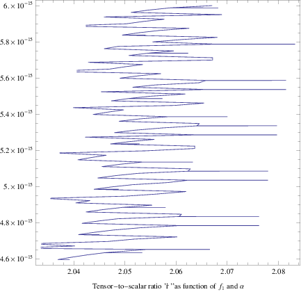
Having the slow-roll indices at hand, one can easily obtain the observational indices (35) in closed form, however we do not quote these here since their final expressions are too lengthy. The phenomenology of the resulting model is interesting, due to the fact that by appropriately adjusting the free parameters , , , and , one can obtain a viable phenomenology, having in mind the constraint on the parameter , which must take values in the range . For example, by choosing , , , and , we obtain and , which are both compatible with the latest Planck Ade:2015lrj and BICEP2/Keck-Array Array:2015xqh data. In the ghost-free model of (21) for the gravity, the inflationary phenomenology is quite interesting and the compatibility with the observational data comes easily without any extreme fine-tuning of the free parameters. In fact, the viability of the theory comes for a wide range of the free parameters. This feature can be seen in Fig. 1 where we present the contour plots of the spectral index (left) and of the tensor-to-scalar ratio (right) as functions of the parameters and for and . Also the rest of the parameters take the value . The blue curves in the left plot correspond to the value and the blue curves in the right plot correspond to .

III.2 Phantom Inflation
Now let us turn our focus on the phantom theory with action given in Eq. (22). For earlier works on -essence phantom theories see Aguirregabiria:2004te and also Refs. Liu:2010dh; Liu:2012iba; Piao:2004tq; Park:2018nfp for general phantom inflation models. We need to note that Also mention that in principle, a phantom theory maybe just an effective description and the complete theory may be free of ghosts.
In the phantom inflation case, if the slow-roll approximation is assumed for the scalar field, the evolution of the phantom scalar is governed by the following differential equation at leading order,
| (39) |
which can be solved and it yields the same solution as in Eq. (29). Let us calculate the slow-roll indices for the model, so after following the steps of the previous section, we obtain the slow-roll indices (III.1), where in the case at hand, the parameters , are,
| (40) |
Accordingly one can easily obtain the observational indices (35) in closed form, which are too lengthy to be presented here. By appropriately adjusting the free parameters , , , and , one can obtain a viable phenomenology, for example, by choosing , , , and , we obtain and , which are both compatible with the latest Planck Ade:2015lrj and BICEP2/Keck-Array Array:2015xqh data. However, it is obvious that extreme fine tuning is needed in the model, nevertheless, a non-viable gravity model becomes viable by the inclusion of an appropriate phantom higher order kinetic scalar field term in the gravitational action. In the next section we shall present a general technique for obtaining viable -essence gravity theories, in the slow-roll approximation.
One issue we did address is the graceful exit from inflation issue in the context of -essence gravity. Essentially from a mathematical point of view, in order to have graceful exit from inflation, the theory needs to have unstable de Sitter solutions (which correspond to an effective equation of state parameter ). This issue seems to depend strongly on the model of gravity chosen, and also depends on the slow-roll condition and it’s implications on the evolution of the scalar field at early times. Formally, this problem can be answered in a concrete way if one analyzes in detail the autonomous dynamical system of the -essence theory, find explicitly the de Sitter attractors and investigate if these are stable or not. Also, the graceful exit from inflation can be achieved by adding terms in the gravitational action, however we do not discuss this issue further in this paper and we hope to address in a more detailed future work.
IV An Alternative Approach to Slow-roll -essence Gravity Inflation
In this section we shall employ a formalism appropriately designed for the -essence gravity models of Eqs. (21) and (22), that will enable us to realize an arbitrarily given evolution and also to test its viability. It is basically a reconstruction technique for the -essence gravity theory (for general reconstruction scheme for -essence, see Matsumoto:2010uv), and we shall provide general formulas that can be used for arbitrary forms of the term. We start off by providing the cosmological evolution we shall be interested to realize with the theory at hand, which in terms of the -foldings number has the following form,
| (41) |
where and are arbitrary parameters of the theory. This cosmological evolution can be realized by specific -essence gravities of the form (21) and (22) which we will now find. To this end we shall appropriately modify the reconstruction technique of Ref. Nojiri:2009kx, to accommodate the -essence term contribution, so we introduce the function , hence the Ricci scalar can be written as follows,
| (42) |
Accordingly, by expressing the functions appearing in the first equation of motion of Eq. (III), and also by using the slow-roll solution of Eq. (29) for the scalar field, we obtain the following differential equation,
| (43) | ||||
where and . Also in the above equation is,
| (44) |
with the plus sign in the last term of Eq. (43), which is the -essence term contribution, corresponding to the phantom case (22) while the minus sign corresponding to the ghost-free theory (21). Given the Hubble rate (41) and by inserting it in Eq. (42) we can find the function which reads,
| (45) |
so accordingly, by using Eq. (45) the differential equation (43) becomes a second order differential equation that can be solved to yield the exact that can realize the cosmological evolution (41). By combining Eqs. (41), (45) and (43), we get the following differential equation,
| (46) |
which can be explicitly solved and it yields the solution,
| (47) |
where and are integration constants, and also the parameters and appearing in Eq. (47) are defined as follows,
| (48) |
Having the gravity which realizes the cosmology (41), we shall use the results of the slow-roll formalism we developed in the previous section for the -essence gravity, and we shall express the slow-roll indices and the corresponding observational indices as functions of the -foldings number.

The formulas we shall produce will enable us to easily test the viability of the resulting theory by confronting it with the observational data of Planck Ade:2015lrj. By using the following formula,
| (49) |
the slow-roll indices of Eq. (33) can be written in terms of the -foldings number, and in the slow-roll approximation these read,
| (50) |
where the prime indicates differentiation with respect to the -foldings number , while the parameters , are defined in Eqs. (III.1) and (III.2) for the ghost-free and for the phantom case respectively. Accordingly, the spectral index and the tensor-to-scalar ratio can be found by the following formulas,
| (51) |
where is equal to,
| (52) |
For the case at hand, the Ricci scalar as a function of reads,
| (53) |
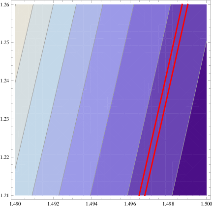
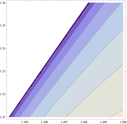
therefore by using the explicit form of the gravity (47) and also by replacing from Eq. (53), we can find the exact form of the slow-roll indices and of the observational indices for both the ghost-free theory (21) and for the phantom theory (22), which we do not quote here for brevity. After a thorough investigation of the parameter space, it can be seen that for the cosmological mode with Hubble rate (41), both the phantom theory can provide a viable phenomenology, in which a simultaneous compatibility of the spectral index and of the tensor-to-scalar ratio with the observational data can be achieved, for a wide range of parameters. For example by using the following values for the free parameters, and by setting the integration constants , we obtain and which are compatible with the Planck data and also with the BICEP2/Keck-Array data. This compatibility occurs for a wide range of the free parameters, as it can be seen for example in Figs. 2 and 3, where we present the contour plots of the spectral index and of the tensor-to-scalar ratio for chosen in the range and for with and . In Fig. 2, the red curves correspond to the values of the spectral index and , which are the maximum and minimum values allowed by the Planck data respectively.

However, the ghost free theory does not provide simultaneous compatibility of and with the observational data. For example if one chooses, , one obtains and which is an unappealing result. However we need to note that the result is model dependent, so for the specific cosmology which has the Hubble rate (41), it seems that the phantom model (22) provides better phenomenology in comparison to the ghost-free model (21).
Therefore, it is possible to produce viable inflationary evolutions in the context of the -essence gravity, by using the slow-roll formalism we presented in this section. Basically, the method we presented is a reconstruction method for realizing inflationary evolutions, in the slow-roll approximation. In principle different types of inflationary evolutions can be realized, but we refrain from going into details because the procedure is the same as the example we presented.
V Conclusions
In this paper we studied a modified gravity theoretical framework which extends the vacuum gravity theory, and it consists of higher order scalar field kinetic terms that are added to the standard gravity Lagrangian density. Due to the form of the extra terms in the action, we called this theory -essence gravity theory, and our main aim was to investigate the inflationary aspects of this theory, in the slow-roll approximation. Actually, the class of -essence gravity theory which we studied in this paper gets very much simplified if the slow-roll condition is imposed on the scalar field, and we investigated the dynamics of inflation in the resulting theory. By using standard formulas for the slow-roll indices coming from generalized theories studied some time ago, we derived the slow-roll indices for a general gravity, and then we applied the formalism for an gravity of the form . This theory without the -essence part is not compatible with the latest Planck observational data, so we questioned the viability of the theory in view of the presence of the -essence terms. As we demonstrated, there is a range of values of the free parameters for which the phenomenological viability of the theory can be achieved, for both the phantom and ghost-free models which we used. Since the result might be model dependent, we used another approach in order to see whether the -essence gravity can produce viable phenomenology. To this end, we fixed the Hubble rate as a function of the -foldings number, and we modified standard gravity reconstruction techniques to accommodate the presence of the -essence terms, always in the slow-roll approximation. Using the resulting reconstruction techniques we derived the -essence gravity which can realize the given Hubble rate, and then we provided general formulas for the slow-roll indices as functions of the -foldings number, always in the slow-roll approximation. Accordingly, we calculated the slow-roll indices and the corresponding observational indices and we demonstrated that the resulting theory can be compatible with the Planck data, however the result is strongly model dependent. Thus we validated that the -essence gravity theory can produce phenomenologically viable cosmologies in the slow-roll approximation. The latter is a vital ingredient of the formalism we employed, so the basic question is, does this theory have inflationary attractors in the absence of the slow-roll condition? The vacuum gravity theory has stable and unstable de Sitter attractors without the slow-roll condition implied, as was explicitly demonstrated in Odintsov:2017tbc, by using the dynamical system approach, so the question is does a general non-slow-roll -essence gravity possesses inflationary attractors? This question is non-trivial and no one can guarantee this, before a consistent autonomous dynamical system is derived for the theory in question. For example, in the case of Gauss-Bonnet gravity there exist inflationary attractors even if the slow-roll condition does not hold true, although these are unstable, as was proved in Ref. Oikonomou:2017ppp, and the same applies for vacuum gravity theories in the presence of a non-flat metric workinprogress. Moreover, the existence of unstable de Sitter attractors is a feature of - theories Kleidis:2018cdx. However the latter type of theory contains potential terms, which are absent in the -essence gravity, so the next major task is to question the existence of inflationary attractors in the non-slow-roll -essence gravity theory. To this end one should appropriately construct a consistent autonomous dynamical system, study its fixed points, and test their stability, analytically if these are hyperbolic fixed points, or at least numerically if the fixed points are non-hyperbolic. The interpretation of the existence of unstable inflationary attractors is a major issue in these theories, which in some sense can be viewed as an inherent mechanism for the graceful exit from inflation, but this is a highly non-trivial issue to discuss here, and of course out of the context of this work. Work is in progress along the above research lines.
Finally, it is noteworthy mentioning that even in this -essence framework, it is unavoidable having the initial Big Bang singularity, when inflationary scenarios are considered. However, it is interesting to note that, if the underlying theory can go beyond the -essence gravity type inflation, namely a torsional based modified gravity Cai:2011tc; Cai:2015emx, or a Horndeski scalar Cai:2012va one may not only realize inflationary cosmology, but also a non-singular bouncing phase that can be applied to avoid the big bang singularity. In fact, it would be interesting to extend the formalism we developed in this paper to find an appropriate -essence gravity type theory that may realize a bouncing cosmology. In the context of other extensions of gravity this is also possible Amoros:2014tha, so the question remains if there are -essence modified gravities that may realize cosmological bounces. We hope to address this issue in a future work.
Acknowledgments
This work is supported by MINECO (Spain), FIS2016-76363-P, and by project 2017 SGR247 (AGAUR, Catalonia) (S.D.O). This work is also supported by MEXT KAKENHI Grant-in-Aid for Scientific Research on Innovative Areas “Cosmic Acceleration” No. 15H05890 (S.N.) and the JSPS Grant-in-Aid for Scientific Research (C) No. 18K03615 (S.N.).
References
- (1) P. A. R. Ade et al. [Planck Collaboration], Astron. Astrophys. 594 (2016) A20 doi:10.1051/0004-6361/201525898 [arXiv:1502.02114 [astro-ph.CO]].
- (2) A. H. Guth, Phys. Rev. D 23 (1981) 347. doi:10.1103/PhysRevD.23.347
- (3) A. A. Starobinsky, Phys. Lett. 91B (1980) 99. doi:10.1016/0370-2693(80)90670-X
- (4) A. D. Linde, Phys. Lett. 129B (1983) 177. doi:10.1016/0370-2693(83)90837-7
- (5) R. Brandenberger and P. Peter, Found. Phys. 47 (2017) no.6, 797 doi:10.1007/s10701-016-0057-0 [arXiv:1603.05834 [hep-th]].
- (6) J. de Haro and Y. F. Cai, Gen. Rel. Grav. 47 (2015) no.8, 95 doi:10.1007/s10714-015-1936-y [arXiv:1502.03230 [gr-qc]].
- (7) Y. F. Cai, Sci. China Phys. Mech. Astron. 57 (2014) 1414 doi:10.1007/s11433-014-5512-3 [arXiv:1405.1369 [hep-th]].
- (8) P. A. R. Ade et al. [BICEP2 and Keck Array Collaborations], Phys. Rev. Lett. 116 (2016) 031302 doi:10.1103/PhysRevLett.116.031302 [arXiv:1510.09217 [astro-ph.CO]].
- (9) S. Nojiri, S. D. Odintsov and V. K. Oikonomou, Phys. Rept. 692 (2017) 1 doi:10.1016/j.physrep.2017.06.001 [arXiv:1705.11098 [gr-qc]].
- (10) S. Nojiri and S. D. Odintsov, Phys. Rept. 505 (2011) 59 doi:10.1016/j.physrep.2011.04.001 [arXiv:1011.0544 [gr-qc]].
- (11) S. Nojiri and S. D. Odintsov, eConf C 0602061 (2006) 06 [Int. J. Geom. Meth. Mod. Phys. 4 (2007) 115] doi:10.1142/S0219887807001928 [hep-th/0601213].
- (12) S. Capozziello and M. De Laurentis, Phys. Rept. 509 (2011) 167 doi:10.1016/j.physrep.2011.09.003 [arXiv:1108.6266 [gr-qc]].
- (13) V. Faraoni and S. Capozziello, Fundam. Theor. Phys. 170 (2010). doi:10.1007/978-94-007-0165-6
- (14) A. de la Cruz-Dombriz and D. Saez-Gomez, Entropy 14 (2012) 1717 doi:10.3390/e14091717 [arXiv:1207.2663 [gr-qc]].
- (15) G. J. Olmo, Int. J. Mod. Phys. D 20 (2011) 413 doi:10.1142/S0218271811018925 [arXiv:1101.3864 [gr-qc]].
- (16) A. Ashtekar and P. Singh, Class. Quant. Grav. 28 (2011) 213001 doi:10.1088/0264-9381/28/21/213001 [arXiv:1108.0893 [gr-qc]].
- (17) A. Ashtekar, T. Pawlowski and P. Singh, Phys. Rev. D 74 (2006) 084003 doi:10.1103/PhysRevD.74.084003 [gr-qc/0607039].
- (18) L. Areste Salo, J. Amoros and J. de Haro, Class. Quant. Grav. 34 (2017) no.23, 235001 doi:10.1088/1361-6382/aa9311 [arXiv:1612.05480 [gr-qc]].
- (19) H. H. Xiong, T. Qiu, Y. F. Cai and X. Zhang, Mod. Phys. Lett. A 24 (2009) 1237 doi:10.1142/S0217732309030667 [arXiv:0711.4469 [hep-th]].
- (20) J. Amoros, J. de Haro and S. D. Odintsov, Phys. Rev. D 89 (2014) no.10, 104010 doi:10.1103/PhysRevD.89.104010 [arXiv:1402.3071 [gr-qc]].
- (21) Y. F. Cai and E. Wilson-Ewing, JCAP 1403 (2014) 026 doi:10.1088/1475-7516/2014/03/026 [arXiv:1402.3009 [gr-qc]].
- (22) J. de Haro and J. Amoros, JCAP 1408 (2014) 025 doi:10.1088/1475-7516/2014/08/025 [arXiv:1403.6396 [gr-qc]].
- (23) K. Kleidis and V. K. Oikonomou, Int. J. Geom. Meth. Mod. Phys. 15 (2018) no.05, 1850071 doi:10.1142/S0219887818500718 [arXiv:1801.02578 [gr-qc]].
- (24) K. Kleidis and V. K. Oikonomou, Int. J. Geom. Meth. Mod. Phys. 15 (2017) no.04, 1850064 doi:10.1142/S0219887818500640 [arXiv:1711.09270 [gr-qc]].
- (25) H. Noh and J. c. Hwang, Phys. Lett. B 515 (2001) 231 doi:10.1016/S0370-2693(01)00875-9 [astro-ph/0107069].
- (26) J. c. Hwang and H. Noh, Phys. Rev. D 71 (2005) 063536 doi:10.1103/PhysRevD.71.063536 [gr-qc/0412126].
- (27) J. c. Hwang and H. Noh, Phys. Rev. D 66 (2002) 084009 doi:10.1103/PhysRevD.66.084009 [hep-th/0206100].
- (28) D. I. Kaiser and E. I. Sfakianakis, Phys. Rev. Lett. 112 (2014) no.1, 011302 doi:10.1103/PhysRevLett.112.011302 [arXiv:1304.0363 [astro-ph.CO]].
- (29) A. A. Starobinsky, Phys. Lett. B 91 (1980) 99 [Phys. Lett. 91B (1980) 99] [Adv. Ser. Astrophys. Cosmol. 3 (1987) 130]. doi:10.1016/0370-2693(80)90670-X
- (30) S. Nojiri, S. D. Odintsov and D. Saez-Gomez, Phys. Lett. B 681 (2009) 74 doi:10.1016/j.physletb.2009.09.045 [arXiv:0908.1269 [hep-th]].
- (31) S. D. Odintsov and V. K. Oikonomou, Phys. Rev. D 96 (2017) no.10, 104049 doi:10.1103/PhysRevD.96.104049 [arXiv:1711.02230 [gr-qc]].
- (32) V. K. Oikonomou, Int. J. Mod. Phys. D 27 (2018) no.05, 1850059 doi:10.1142/S0218271818500591 [arXiv:1711.03389 [gr-qc]].
- (33) Work in progress.
- (34) K. Kleidis and V. K. Oikonomou, arXiv:1808.04674 [gr-qc].
- (35) T. Chiba, T. Okabe and M. Yamaguchi, Phys. Rev. D 62 (2000) 023511 doi:10.1103/PhysRevD.62.023511 [astro-ph/9912463].
- (36) C. Armendariz-Picon, V. F. Mukhanov and P. J. Steinhardt, Phys. Rev. Lett. 85 (2000) 4438 doi:10.1103/PhysRevLett.85.4438 [astro-ph/0004134].
- (37) C. Armendariz-Picon, T. Damour and V. F. Mukhanov, Phys. Lett. B 458 (1999) 209 doi:10.1016/S0370-2693(99)00603-6 [hep-th/9904075].
- (38) J. Matsumoto and S. Nojiri, Phys. Lett. B 687 (2010) 236 doi:10.1016/j.physletb.2010.03.030 [arXiv:1001.0220 [hep-th]].
- (39) C. Armendariz-Picon, V. F. Mukhanov and P. J. Steinhardt, Phys. Rev. D 63 (2001) 103510 doi:10.1103/PhysRevD.63.103510 [astro-ph/0006373].
- (40) T. Chiba, Phys. Rev. D 66 (2002) 063514 doi:10.1103/PhysRevD.66.063514 [astro-ph/0206298].
- (41) M. Malquarti, E. J. Copeland, A. R. Liddle and M. Trodden, Phys. Rev. D 67 (2003) 123503 doi:10.1103/PhysRevD.67.123503 [astro-ph/0302279].
- (42) M. Malquarti, E. J. Copeland and A. R. Liddle, Phys. Rev. D 68 (2003) 023512 doi:10.1103/PhysRevD.68.023512 [astro-ph/0304277].
- (43) L. P. Chimento and A. Feinstein, Mod. Phys. Lett. A 19 (2004) 761 doi:10.1142/S0217732304013507 [astro-ph/0305007].
- (44) L. P. Chimento, Phys. Rev. D 69 (2004) 123517 doi:10.1103/PhysRevD.69.123517 [astro-ph/0311613].
- (45) R. J. Scherrer, Phys. Rev. Lett. 93 (2004) 011301 doi:10.1103/PhysRevLett.93.011301 [astro-ph/0402316].
- (46) J. M. Aguirregabiria, L. P. Chimento and R. Lazkoz, Phys. Rev. D 70 (2004) 023509 doi:10.1103/PhysRevD.70.023509 [astro-ph/0403157].
- (47) C. Armendariz-Picon and E. A. Lim, JCAP 0508 (2005) 007 doi:10.1088/1475-7516/2005/08/007 [astro-ph/0505207].
- (48) L. R. Abramo and N. Pinto-Neto, Phys. Rev. D 73 (2006) 063522 doi:10.1103/PhysRevD.73.063522 [astro-ph/0511562].
- (49) A. D. Rendall, Class. Quant. Grav. 23 (2006) 1557 doi:10.1088/0264-9381/23/5/008 [gr-qc/0511158].
- (50) J. P. Bruneton, Phys. Rev. D 75 (2007) 085013 doi:10.1103/PhysRevD.75.085013 [gr-qc/0607055].
- (51) R. de Putter and E. V. Linder, Astropart. Phys. 28 (2007) 263 doi:10.1016/j.astropartphys.2007.05.011 [arXiv:0705.0400 [astro-ph]].
- (52) E. Babichev, V. Mukhanov and A. Vikman, JHEP 0802 (2008) 101 doi:10.1088/1126-6708/2008/02/101 [arXiv:0708.0561 [hep-th]].
- (53) C. Deffayet, X. Gao, D. A. Steer and G. Zahariade, Phys. Rev. D 84 (2011) 064039 doi:10.1103/PhysRevD.84.064039 [arXiv:1103.3260 [hep-th]].
- (54) N. Kan, K. Shiraishi and M. Yashiki, arXiv:1811.11967 [gr-qc].
- (55) Z. G. Liu, J. Zhang and Y. S. Piao, Phys. Lett. B 697 (2011) 407 doi:10.1016/j.physletb.2010.12.055 [arXiv:1012.0673 [gr-qc]].
- (56) Z. G. Liu and Y. S. Piao, Phys. Lett. B 713 (2012) 53 doi:10.1016/j.physletb.2012.05.027 [arXiv:1203.4901 [gr-qc]].
- (57) Y. S. Piao and Y. Z. Zhang, Phys. Rev. D 70 (2004) 063513 doi:10.1103/PhysRevD.70.063513 [astro-ph/0401231].
- (58) S. Park and R. P. Woodard, arXiv:1809.06841 [gr-qc].
- (59) Y. F. Cai, S. H. Chen, J. B. Dent, S. Dutta and E. N. Saridakis, Class. Quant. Grav. 28 (2011) 215011 doi:10.1088/0264-9381/28/21/215011 [arXiv:1104.4349 [astro-ph.CO]].
- (60) Y. F. Cai, S. Capozziello, M. De Laurentis and E. N. Saridakis, Rept. Prog. Phys. 79 (2016) no.10, 106901 doi:10.1088/0034-4885/79/10/106901 [arXiv:1511.07586 [gr-qc]].
- (61) Y. F. Cai, D. A. Easson and R. Brandenberger, JCAP 1208 (2012) 020 doi:10.1088/1475-7516/2012/08/020 [arXiv:1206.2382 [hep-th]].
- (62) J. Amoros, J. de Haro and S. D. Odintsov, Phys. Rev. D 89 (2014) no.10, 104010 doi:10.1103/PhysRevD.89.104010 [arXiv:1402.3071 [gr-qc]].