跳到论文正文
W Papers独立论文阅读器 arXiv:1902.03552 论文正文 计算阅读时间 · 0%
引用这篇论文根据当前论文元数据生成,正式投稿前建议核对。


License: arXiv.org perpetual non-exclusive license
arXiv:1902.03552v4 [cs.IT] 11 May 2021

Sampling and Remote Estimation for the Ornstein-Uhlenbeck Process through Queues: Age of Information and BeyondThanks: Tasmeen Zaman Ornee and Yin Sun are with Dept. of ECE, Auburn University, Auburn, AL (emails: tzo0017@auburn.edu, yzs0078@auburn.edu).Thanks: This work was supported in part by NSF grant CCF-1813050 and ONR grant N00014-17-1-2417.

Tasmeen Zaman Ornee    Student Member, IEEE    Yin Sun    Senior Member, IEEE Affiliation: 
Abstract

Recently, a connection between the age of information and remote estimation error was found in a sampling problem of Wiener processes: If the sampler has no knowledge of the signal being sampled, the optimal sampling strategy is to minimize the age of information; however, by exploiting causal knowledge of the signal values, it is possible to achieve a smaller estimation error. In this paper, we generalize the previous study by investigating a problem of sampling a stationary Gauss-Markov process named the Ornstein-Uhlenbeck (OU) process, where we aim to find useful insights for solving the problems of sampling more general signals. The optimal sampling problem is formulated as a constrained continuous-time Markov decision process (MDP) with an uncountable state space. We provide an exact solution to this MDP: The optimal sampling policy is a threshold policy on instantaneous estimation error and the threshold is found. Further, if the sampler has no knowledge of the OU process, the optimal sampling problem reduces to an MDP for minimizing a nonlinear age of information metric. The age-optimal sampling policy is a threshold policy on expected estimation error and the threshold is found. In both problems, the optimal sampling policies can be computed by low-complexity algorithms (e.g., bisection search and Newton’s method), and the curse of dimensionality is circumvented. These results hold for (i) general service time distributions of the queueing server and (ii) sampling problems both with and without a sampling rate constraint. Numerical results are provided to compare different sampling policies.

Index Terms: 
Age of information, Ornstein-Uhlenbeck process, sampling policy, threshold policy.

I Introduction

Timely updates of the system state are of significant importance for state estimation and decision making in networked control and cyber-physical systems, such as UAV navigation, robotics control, mobility tracking, and environment monitoring systems. To evaluate the freshness of state updates, the concept of Age of Information, or simply age, was introduced to measure the timeliness of state samples received from a remote transmitter [1, 2, 3]. Let UtU_{t} be the generation time of the freshest received state sample at time tt. The age of information, as a function of tt, is defined as Δt=t−Ut\Delta_{t}=t-U_{t}, which is the time difference between the freshest samples available at the transmitter and receiver.

Recently, the age of information concept has received significant attention, because of the extensive applications of state updates among systems connected over communication networks. The states of many systems, such as UAV mobility trajectory and sensor measurements, are in the form of a signal XtX_{t}, that may change slowly at some time and vary more dynamically later. Hence, the time difference described by the age Δt=t−Ut\Delta_{t}=t-U_{t} only partially characterize the variation Xt−XUtX_{t}-X_{U_{t}} of the system state, and the state update policy that minimizes the age of information does not minimize the state estimation error. This result was first shown in [4], where a sampling problem of Wiener processes was solved and the optimal sampling policy was shown to have an intuitive structure. As the results therein hold only for signals that can be modeled as a Wiener process, one would wonder how to, and whether it is possible to, extend [4] for handling more general signal models.

In this paper, we generalize [4] by exploring a problem of sampling an Ornstein-Uhlenbeck (OU) process XtX_{t}. From the obtained results, we hope to find useful structural properties of the optimal sampler design that can be potentially applied to more general signal models. The OU process XtX_{t} is the continuous-time analogue of the well-known first-order autoregressive process, i.e., AR(1) process. The OU process is defined as the solution to the stochastic differential equation (SDE) [5, 6]

d​Xt=θ⁡(μ−Xt)​d​t+σ​d​Wt,\displaystyle dX_{t}=\theta(\mu-X_{t})dt+\sigma dW_{t}, (1)

where μ\mu, θ>0\theta>0, and σ>0\sigma>0 are parameters and WtW_{t} represents a Wiener process. It is the only nontrivial continuous-time process that is stationary, Gaussian, and Markovian [6]. Examples of first-order systems that can be described as the OU process include interest rates, currency exchange rates, and commodity prices (with modifications) [7], control systems such as node mobility in mobile ad-hoc networks, robotic swarms, and UAV systems [8, 9], and physical processes such as the transfer of liquids or gases in and out of a tank [10].

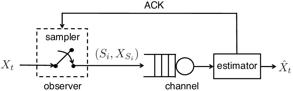
As shown in Fig. 1, samples of an OU process are forwarded to a remote estimator through a channel in a first-come, first-served (FCFS) fashion. The samples experience i.i.d. random transmission times over the channel, which is caused by random sample size, channel fading, interference, congestions, and etc. For example, UAVs flying close to WiFi access points may suffer from long communication delay and instability issues, because they receive strong interference from the WiFi access points [11]. We assume that at any time only one sample can be served by the channel. The samples that are waiting to be sent are stored in a queue at the transmitter. Hence, the channel is modeled as an FCFS queue with i.i.d. service times. The service time distributions considered in this paper are quite general: they are only required to have a finite mean. This queueing model is helpful to analyze the robustness of remote estimation systems with occasionally long transmission times.
Refer to caption
Fig. 1: System model.

The estimator utilizes causally received samples to construct an estimate X^t\hat{X}_{t} of the real-time signal value XtX_{t}. The quality of remote estimation is measured by the time-average mean-squared estimation error, i.e.,

𝗆𝗌𝖾=lim supT→∞1T​𝔼​[∫0T(Xt−X^t)2​𝑑t].\displaystyle{\mathsf{mse}}=\limsup_{T\rightarrow\infty}\frac{1}{T}\mathbb{E}\left[\int_{0}^{T}(X_{t}-\hat{X}_{t})^{2}dt\right]. (2)

Our goal is to find the optimal sampling policy that minimizes 𝗆𝗌𝖾\mathsf{mse} by causally choosing the sampling times subject to a maximum sampling rate constraint. In practice, the cost (e.g., energy, CPU cycle, storage) for state updates increases with the average sampling rate. Hence, we are striking to find the optimum tradeoff between estimation error and update cost. In addition, the unconstrained problem is also solved. The contributions of this paper are summarized as follows:

  • •

    The optimal sampling problem for minimize the 𝗆𝗌𝖾{\mathsf{mse}} under a sampling rate constraint is formulated as a constrained continuous-time Markov decision process (MDP) with an uncountable state space. Because of the curse of dimensionality, such problems are often lack of low-complexity solutions that are arbitrarily accurate. However, we were able to solve this MDP exactly: The optimal sampling policy is proven to be a threshold policy on instantaneous estimation error, where the threshold is a non-linear function v⁡(β)v(\beta) of a parameter β\beta. The value of β\beta is equal to the summation of the optimal objective value of the MDP and the optimal Lagrangian dual variable associated to the sampling rate constraint. If there is no sampling rate constraint, the Lagrangian dual variable is zero and hence β\beta is exactly the optimal objective value. Among the technical tools developed to prove this result is a free boundary method [12], [13] for finding the optimal stopping time of the OU process.

  • •

    The optimal sampler design of Wiener process in [4] is a limiting case of the above result. By comparing the optimal sampling policies of OU process and Wiener process, we find that the threshold function v⁡(β)v(\beta) changes according to the signal model, where the parameter β\beta is determined in the same way for both signal models.

  • •

    Further, we consider a class of signal-agnostic sampling policies, where the sampling times are determined without using knowledge of the signal value of the observed OU process; the parameters of the OU process are known. The optimal signal-agnostic sampling problem is equivalent to an MDP for minimizing the time-average of a nonlinear age function p⁡(Δt)p(\Delta_{t}), which has been solved recently in [14]. The age-optimal sampling policy is a threshold policy on expected estimation error, where the threshold function is simply v⁡(β)=βv(\beta)=\beta and the parameter β\beta is determined in the same way as above.

  • •

    The above results hold for (i) general service time distributions with a finite mean and (ii) sampling problems both with and without a sampling rate constraint. Numerical results suggest that the optimal sampling policy is better than zero-wait sampling and the classic uniform sampling.

One interesting observation from these results is that the threshold function v⁡(β)v(\beta) varies with respect to the signal model and sampling problem, but the parameter β\beta is determined in the same way.

I-A Related Work

The results in this paper are tightly related to recent studies on the age of information Δt\Delta_{t}, e.g., [1, 15, 14, 16, 17, 18, 19, 20, 21, 22, 23, 24, 25, 26, 27, 28, 29, 30, 31, 32, 33, 34, 35], which does not have a signal model. The average age and average peak age have been analyzed for various queueing systems in, e.g., [1, 18, 20, 21]. The optimality of the Last-Come, First-Served (LCFS) policy, or more generally the Last-Generated, First-Served (LGFS) policy, was established for various queueing system models in [24, 25, 26, 30]. Optimal sampling policies for minimizing non-linear age functions were developed in, e.g., [19, 15, 14, 35]. Age-optimal transmission scheduling of wireless networks were investigated in, e.g., [22, 23, 27, 28, 29, 31, 32].

On the other hand, this paper is also a contribution to the area of remote estimation, e.g., [36, 10, 37, 38, 39, 40, 41]. In [37, 39], optimal sampling of Wiener processes was studied, where the transmission time from the sampler to the estimator is zero. Optimal sampling of OU processes was also considered in [37], which is solved by discretizing time and using dynamic programming to solve the discrete-time optimal stopping problems. However, our optimal sampler of OU processes is obtained analytically. Remote estimation over several different channel models was recently studied in, e.g., [40, 41]. In [36, 10, 37, 38, 39, 40, 41], the optimal sampling policies were proven to be threshold policies. Because of the queueing model, our optimal sampling policy has a different structure from those in [36, 10, 37, 38, 39, 40, 41]. Specifically, in our optimal sampling policy, sampling is suspended when the server is busy and is reactivated once the server becomes idle. In addition, we are able to characterize the threshold precisely. The optimal sampling policy for the Wiener process in [4] is a limiting case of ours. Remote estimation of the Wiener process with random two-way delay was recently considered in [42]. In [43], a jointly optimal sampler, quantizer, and estimator design was found for a class of continuous-time Markov processes under a bit-rate constraint. A recent survey on remote estimation systems was presented in [44].

II Model and Formulation

II-A System Model

We consider the remote estimation system illustrated in Fig. 1, where an observer takes samples from an OU process XtX_{t} and forwards the samples to an estimator through a communication channel. The channel is modeled as a single-server FCFS queue with i.i.d. service times. The system starts to operate at time t=0t=0. The ii-th sample is generated at time SiS_{i} and is delivered to the estimator at time DiD_{i} with a service time YiY_{i}, which satisfy Si≤Si+1S_{i}\leq S_{i+1}, Si+Yi≤DiS_{i}+Y_{i}\leq D_{i}, Di+Yi+1≤Di+1D_{i}+Y_{i+1}\leq D_{i+1}, and 0<𝔼⁡[Yi]<∞0<\mathbb{E}[Y_{i}]<\infty for all ii. Each sample packet (Si,XSi)(S_{i},X_{S_{i}}) contains the sampling time SiS_{i} and the sample value XSiX_{S_{i}}. Let Ut=max⁡{Si:Di≤t}U_{t}=\max\{S_{i}:D_{i}\leq t\} be the sampling time of the latest received sample at time tt. The age of information, or simply age, at time tt is defined as [1, 2]

Δt=t−Ut=t−max⁡{Si:Di≤t},\displaystyle\Delta_{t}=t-U_{t}=t-\max\{S_{i}:D_{i}\leq t\}, (3)

which is shown in Fig. 2. Because Di≤Di+1D_{i}\leq D_{i+1}, Δt\Delta_{t} can be also expressed as

Δt=t−Si,ift∈[Di,Di+1),i=0,1,2,…\displaystyle\Delta_{t}=t-S_{i},~\text{if}~t\in[D_{i},D_{i+1}),~i=0,1,2,\ldots (4)

The initial state of the system is assumed to satisfy S0=0S_{0}=0, D0=Y0D_{0}=Y_{0}, X0X_{0} and Δ0\Delta_{0} are finite constants. The parameters μ\mu, θ\theta, and σ\sigma in (1) are known at both the sampler and estimator.

Let It∈{0,1}I_{t}\in\{0,1\} represent the idle/busy state of the server at time tt. We assume that whenever a sample is delivered, an acknowledgement is sent back to the sampler with zero delay. By this, the idle/busy state ItI_{t} of the server is known at the sampler. Therefore, the information that is available at the sampler at time tt can be expressed as {Xs,Is:0≤s≤t}\{X_{s},I_{s}:0\leq s\leq t\}.

ttΔt\Delta_{t}S0S_{0}S1S_{1}Sj−1S_{j-1}SjS_{j}D0D_{0}D1D_{1}Dj−1D_{j-1}DjD_{j}
Fig. 2: Evolution of the age Δt\Delta_{t} over time.

II-B Sampling Policies

In causal sampling policies, each sampling time SiS_{i} is determined based on the up-to-date information that is available at the sampler, without using any future information. In probability theory, such sampling times are represented by stopping times.

To define stopping time precisely, the concepts of σ\sigma-field and filtration are needed. Let us define the σ\sigma-field

𝒩t\displaystyle\mathcal{N}_{t} =σ(Xs,Is:0≤s≤t),\displaystyle=\sigma(X_{s},I_{s}:0\leq s\leq t),

which is the set of events whose occurrence are determined by the realization of the process {Xs,Is,0≤s≤t}\{X_{s},I_{s},0\leq s\leq t\} up to time tt. A filtration is a non-decreasing sequence of σ\sigma-fields. Our analysis requires a strong Markov property, which is satisfied when the filtration is right-continuous. Define

𝒩t+=∩s>t𝒩s,\displaystyle\mathcal{N}_{t}^{+}=\cap_{s>t}\mathcal{N}_{s}, (5)

then {𝒩t+,t≥0}\{\mathcal{N}_{t}^{+},t\geq 0\} is a right-continuous filtration of the information process {Xs,Is,t≥0}\{X_{s},I_{s},t\geq 0\} [45]. In a causal sampling policy, each sampling time is a stopping time with respect to {𝒩t+,t≥0}\{\mathcal{N}_{t}^{+},t\geq 0\}, i.e.,

{Si≤t}∈𝒩t+,∀t≥0.\displaystyle\{S_{i}\leq t\}\in\mathcal{N}_{t}^{+},~\forall t\geq 0. (6)

In other words, whether sample ii has been generated by time tt (i.e., whether {Si≤tS_{i}\leq t} or {Si>tS_{i}>t}) is determined by the realization of the process {Xs,Is,0≤s≤t}\{X_{s},I_{s},0\leq s\leq t\} up to time tt.

Let π=(S1,S2,…)\pi=(S_{1},S_{2},...) represent a sampling policy. We use Π\Pi to represent the set of causal sampling policies that satisfy two conditions: (i) Each sampling policy π∈Π\pi\in\Pi satisfies (6) for all ii. (ii) The sequence of inter-sampling times {Ti=Si+1−Si,i=0,1,…}\{T_{i}=S_{i+1}-S_{i},i=0,1,\ldots\} forms a regenerative process [46, Section 6.1]: There exists an increasing sequence 0≤k1<k2<…0\leq{k_{1}}<k_{2}<\ldots of almost surely finite random integers such that the post-kj{k_{j}} process {Tkj+i,i=0,1,…}\{T_{k_{j}+i},i=0,1,\ldots\} has the same distribution as the post-k0{k_{0}} process {Tk0+i,i=0,1,…}\{T_{k_{0}+i},i=0,1,\ldots\} and is independent of the pre-kjk_{j} process {Ti,i=0,1,…,kj−1}\{T_{i},i=0,1,\ldots,k_{j}-1\}; further, we assume that 𝔼⁡[kj+1−kj]<∞\mathbb{E}[{k_{j+1}}-{k_{j}}]<\infty, 𝔼⁡[Sk1]<∞\mathbb{E}[S_{k_{1}}]<\infty, and 0<𝔼[Skj+1−Skj]<∞,j=1,2,…0<\mathbb{E}[S_{k_{j+1}}-S_{k_{j}}]<\infty,~j=1,2,\ldots11 1 We will optimize lim supT→∞𝔼⁡[∫0T(Xt−X^t)2​𝑑t]/T\limsup_{T\rightarrow\infty}\mathbb{E}[\int_{0}^{T}(X_{t}-\hat{X}_{t})^{2}dt]/T, but operationally a nicer criterion is lim supi→∞𝔼⁡[∫0Di(Xt−X^t)2​𝑑t]/𝔼⁡[Di]\limsup_{i\rightarrow\infty}\mathbb{E}[\int_{0}^{D_{i}}(X_{t}-\hat{X}_{t})^{2}dt]/{\mathbb{E}[D_{i}]}. These criteria are corresponding to two definitions of “average cost per unit time” that are widely used in the literature of semi-Markov decision processes. These two criteria are equivalent, if {T1,T2,…}\{T_{1},T_{2},\ldots\} is a regenerative process, or more generally, if {T1,T2,…}\{T_{1},T_{2},\ldots\} has only one ergodic class. If not condition is imposed, however, they are different. The interested readers are referred to [47, 48, 49, 50, 51] for more discussions.

From this, we can obtain that SiS_{i} is finite almost surely for all ii. We assume that the OU process {Xt,t≥0}\{X_{t},t\geq 0\} and the service times {Yi,i=1,2,…}\{Y_{i},i=1,2,\dots\} are mutually independent, and do not change according to the sampling policy.

A sampling policy π∈Π\pi\in\Pi is said to be signal-agnostic (signal-aware), if π\pi is (not necessarily) independent of {Xt,t≥0}\{X_{t},t\geq 0\}. Let Πsignal-agnostic⊂Π\Pi_{\text{signal-agnostic}}\subset\Pi denote the set of signal-agnostic sampling policies, defined as

Πsignal-agnostic={π∈Π:π​ is independent of ​{Xt,t≥0}}.\displaystyle\!\!\Pi_{\text{signal-agnostic}}\!=\!\{\pi\!\in\Pi:\pi\text{ is independent of }\{X_{t},t\geq 0\}\}.\!\!\! (7)

II-C MMSE Estimator

According to (6), SiS_{i} is a finite stopping time. By using [52, Eq. (3)] and the strong Markov property of the OU process [12, Eq. (4.3.27)], XtX_{t} is expressed as

Xt=\displaystyle X_{t}= XSi​e−θ⁡(t−Si)+μ⁡[1−e−θ⁡(t−Si)]\displaystyle X_{S_{i}}e^{-\theta(t-S_{i})}+\mu\big[1-e^{-\theta(t-S_{i})}\big]
+σ2​θ​e−θ⁡(t−Si)​We2​θ​(t−Si)−1, if ​t∈[Si,∞).\displaystyle+\frac{\sigma}{\sqrt{2\theta}}e^{-\theta(t-S_{i})}W_{e^{2\theta(t-S_{i})}-1},\text{ if }t\in[S_{i},\infty). (8)

At any time t≥0t\geq 0, the estimator uses causally received samples to construct an estimate X^t\hat{X}_{t} of the real-time signal value XtX_{t}. The information available to the estimator consists of two parts: (i) Mt={(Si,XSi,Di):Di≤t}M_{t}=\{(S_{i},X_{S_{i}},D_{i}):D_{i}\leq t\}, which contains the sampling time SiS_{i}, sample value XSiX_{S_{i}}, and delivery time DiD_{i} of the samples that have been delivered by time tt and (ii) the fact that no sample has been received after the last delivery time max⁡{Di:Di≤t}\max\{D_{i}:D_{i}\leq t\}. Similar to [37, 53, 4], we assume that the estimator neglects the second part of information.22 2 We note that this assumption can be removed by considering a joint sampler and estimator design problem. Specifically, it was shown in [36, 10, 38, 40, 41] that when the sampler and estimator are jointly optimized in discrete-time systems, the optimal estimator has the same expression no matter with or without the second part of information. As pointed out in [36, p. 619], such a structure property of the MMSE estimator can be also established for continuous-time systems. The goal of this paper is to find the closed-form expression of the optimal sampler under this assumption. The remaining task of finding the jointly optimal sampler and estimator design can be done by further using the majorization techniques developed in [36, 10, 38, 40, 41]; see [43] for a recent treatment on this task. Then, as shown in Appendix C, the minimum mean square error (MMSE) estimator is determined by

X^t=𝔼⁡[Xt|Mt]=\displaystyle\hat{X}_{t}=\mathbb{E}[{X}_{t}|M_{t}]= XSi​e−θ⁡(t−Si)+μ⁡[1−e−θ⁡(t−Si)],\displaystyle X_{S_{i}}e^{-\theta(t-S_{i})}+\mu\big[1-e^{-\theta(t-S_{i})}\big],
ift∈[Di,Di+1),i=0,1,2,…\displaystyle\text{if}~t\in[D_{i},D_{i+1}),~i=0,1,2,\ldots (9)

Hence, the estimation error of the MMSE estimator is

Xt−X^t=\displaystyle X_{t}-\hat{X}_{t}= σ2​θ​e−θ​t​We2​θ​t−1,\displaystyle\frac{\sigma}{\sqrt{2\theta}}e^{-\theta t}W_{e^{2\theta t}-1},
ift∈[Di,Di+1),i=0,1,2,…\displaystyle\text{if}~t\in[D_{i},D_{i+1}),i=0,1,2,\ldots\!\!\!\!\!\!\!\!\!\!\!\! (10)

II-D Problem Formulation

The goal of this paper is to find the optimal sampling policy that minimizes the mean-squared estimation error subject to an average sampling-rate constraint, which is formulated as the following problem:

𝗆𝗌𝖾opt=infπ∈Π\displaystyle{\mathsf{mse}}_{\text{opt}}=\inf_{\pi\in\Pi}~ lim supT→∞1T​𝔼​[∫0T(Xt−X^t)2​𝑑t]\displaystyle\limsup_{T\rightarrow\infty}\frac{1}{T}\mathbb{E}\left[\int_{0}^{T}(X_{t}-\hat{X}_{t})^{2}dt\right] (11)
 s.t.  lim infn→∞1n​𝔼​[∑i=1n(Si+1−Si)]≥1fmax,\displaystyle\liminf_{n\rightarrow\infty}\frac{1}{n}\mathbb{E}\left[\sum_{i=1}^{n}(S_{i+1}-S_{i})\right]\geq\frac{1}{f_{\max}}, (12)

where 𝗆𝗌𝖾opt{\mathsf{mse}}_{\text{opt}} is the optimum value of (11) and fmaxf_{\max} is the maximum allowed sampling rate. When fmax=∞f_{\max}=\infty, this problem becomes an unconstrained problem.

III Main Results

III-A Signal-aware Sampling without Rate Constraint

Problem (11) is a constrained continuous-time MDP with a continuous state space. However, we found an exact solution to this problem. To present this solution, let us consider an OU process OtO_{t} with the initial state Ot=0O_{t}=0 and parameter μ=0\mu=0. According to (II-C), OtO_{t} can be expressed as

Ot=σ2​θ​e−θ​t​We2​θ​t−1.\displaystyle O_{t}=\frac{\sigma}{\sqrt{2\theta}}e^{-\theta t}W_{e^{2\theta t}-1}. (13)

Define

𝗆𝗌𝖾Yi=𝔼⁡[OYi2]=σ22​θ​𝔼​[1−e−2​θ​Yi],\displaystyle\mathsf{mse}_{Y_{i}}=\mathbb{E}[O_{Y_{i}}^{2}]=\frac{\sigma^{2}}{2\theta}\mathbb{E}[1-e^{-{2\theta{Y_{i}}}}], (14)
𝗆𝗌𝖾∞=𝔼⁡[O∞2]=σ22​θ.\displaystyle\mathsf{mse}_{\infty}=\mathbb{E}[O_{\infty}^{2}]=\frac{\sigma^{2}}{2\theta}. (15)

In the sequel, we will see that 𝗆𝗌𝖾Yi\mathsf{mse}_{Y_{i}} and 𝗆𝗌𝖾∞\mathsf{mse}_{\infty} are the lower and upper bounds of 𝗆𝗌𝖾opt\mathsf{mse}_{\text{opt}}, respectively. According to (II-C) and (13)-(15), 𝗆𝗌𝖾Yi\mathsf{mse}_{Y_{i}} represents the estimation error when the estimation is made based on a sample that was generated YiY_{i} seconds ago, and 𝗆𝗌𝖾∞\mathsf{mse}_{\infty} represents the estimation error for the case that no sample has been delivered to the estimator before. We will also need to use the function33 3 If x=0x=0, G⁡(x)G(x) is defined as its right limit G⁡(0)=limx→0+G⁡(x)=1G(0)=\lim_{x\rightarrow 0^{+}}G(x)=1.

G⁡(x)=ex2x​∫0xe−t2​𝑑t=ex2x​π2​erf​(x),x∈[0,∞),\displaystyle G(x)=\!\!\frac{e^{x^{2}}}{x}{\int_{0}^{x}e^{-{t^{2}}}dt}\!\!\thinspace=\thinspace\frac{e^{x^{2}}}{x}\frac{\sqrt{\pi}}{2}\thinspace{\text{erf}}(x),~x\in[0,\infty), (16)

where erf​(⋅)\text{erf}(\cdot) is the error function [54], defined as

erf​(x)=2π​∫0xe−t2​𝑑t.\displaystyle{\text{erf}}(x)=\frac{2}{\sqrt{\pi}}\int_{0}^{x}e^{-t^{2}}dt. (17)

We first consider the unconstrained optimal sampling problem, i.e., fmax=∞f_{\max}={\infty}, such that the rate constraint (12) can be removed. In this scenario, the optimal sampler is provided in the following theorem.

Theorem 1.

(Sampling without Rate Constraint). If fmax=∞f_{\max}={\infty} and the YiY_{i}’s are i.i.d. with 0<𝔼⁡[Yi]<∞0<\mathbb{E}[Y_{i}]<\infty, then (S1​(β),S2​(β),…)(S_{1}(\beta),S_{2}(\beta),\ldots) with a parameter β\beta is an optimal solution to (11), where

Si+1​(β)=inf{t≥Di​(β):|Xt−X^t|≥v⁡(β)},\displaystyle S_{i+1}(\beta)=\inf\left\{t\geq D_{i}(\beta):\!\big|X_{t}-\hat{X}_{t}\big|\!\geq\!{v}(\beta)\right\}, (18)

Di​(β)=Si​(β)+YiD_{i}(\beta)=S_{i}(\beta)+Y_{i}, v⁡(β){v}(\beta) is defined by

v⁡(β)=σθ​G−1​(𝗆𝗌𝖾∞−𝗆𝗌𝖾Yi𝗆𝗌𝖾∞−β),\displaystyle{v}(\beta)=\frac{\sigma}{\sqrt{\theta}}G^{-1}\left(\frac{\mathsf{mse}_{\infty}-\mathsf{mse}_{Y_{i}}}{\mathsf{mse}_{\infty}-{\beta}}\right), (19)

G−1​(⋅)G^{-1}(\cdot) is the inverse function of G⁡(⋅)G(\cdot) in (16) and β\beta is the unique root of

𝔼⁡[∫Di​(β)Di+1​(β)(Xt−X^t)2​𝑑t]−β​𝔼​[Di+1​(β)−Di​(β)]=\displaystyle\!\!\!\mathbb{E}\left[\int_{D_{i}(\beta)}^{D_{i+1}(\beta)}(X_{t}-\hat{X}_{t})^{2}dt\right]\!-\!{\beta}{\mathbb{E}[D_{i+1}(\beta)\!-\!D_{i}(\beta)]}\!=\!0.\!\!\! (20)

The optimal objective value to (11) is given by

𝗆𝗌𝖾opt=𝔼⁡[∫Di​(β)Di+1​(β)(Xt−X^t)2​𝑑t]𝔼⁡[Di+1​(β)−Di​(β)].\displaystyle\mathsf{mse}_{\text{opt}}=\frac{\mathbb{E}\left[\int_{D_{i}(\beta)}^{D_{i+1}(\beta)}\!(X_{t}-\hat{X}_{t})^{2}dt\right]}{\mathbb{E}[D_{i+1}(\beta)\!-\!D_{i}(\beta)]}.{\noindent} (21)

​​Furthermore, β\beta is exactly the optimal value to (11), i.e., β=𝗆𝗌𝖾opt{\beta}={\mathsf{mse}}_{\text{opt}}.

The proof of Theorem 1 is explained in Section IV. The optimal sampling policy in Theorem 1 has a nice structure. Specifically, the (i+1)(i+1)-th sample is taken at the earliest time tt satisfying two conditions: (i) The ii-th sample has already been delivered by time tt, i.e., t≥Di​(β)t\geq D_{i}(\beta), and (ii) the estimation error |Xt−X^t||X_{t}-\hat{X}_{t}| is no smaller than a pre-determined threshold v⁡(β){v}(\beta), where v⁡(⋅)v(\cdot) is a non-linear function defined in (19). In Section IV, it is shown that 𝗆𝗌𝖾Yi≤β<𝗆𝗌𝖾∞\mathsf{mse}_{Y_{i}}\leq\beta<\mathsf{mse}_{\infty}. Further, it is not hard to show that G⁡(x)G(x) is strictly increasing on [0,∞)[0,\infty) and G⁡(0)=1G(0)=1. Hence, its inverse function G−1​(⋅)G^{-1}(\cdot) and the threshold v⁡(β)v(\beta) are properly defined and v⁡(β)≥0v(\beta)\geq 0.

III-A1 Three Algorithms for Solving (20)

We now present three algorithms for computing the root of (20). Because the Si​(β)S_{i}(\beta)’s are stopping times, numerically calculating the expectations in (20) appears to be a difficult task. Nonetheless, this challenge can be solved by resorting to the following lemma, which is obtained by using Dynkin’s formula [13, Theorem 7.4.1] and the optional stopping theorem.

Refer to caption
Fig. 3: f⁡(β)f(\beta) in (30) for i.i.d. exponential service time with 𝔼⁡[Yi]=1\mathbb{E}[Y_{i}]=1, where the parameters of the OU process are σ=1\sigma=1 and θ=0.5\theta=0.5. For these parameters, 𝗆𝗌𝖾Yi=0.5\mathsf{mse}_{Y_{i}}=0.5 and 𝗆𝗌𝖾∞=1\mathsf{mse}_{\infty}=1.
Lemma 1.

In Theorem 1, it holds that

𝔼⁡[Di+1​(β)−Di​(β)]\displaystyle\mathbb{E}[D_{i+1}(\beta)-D_{i}(\beta)]
=\displaystyle= 𝔼⁡[max⁡{R1​(v⁡(β))−R1​(OYi),0}]+𝔼⁡[Yi],\displaystyle\mathbb{E}[\max\{R_{1}(v(\beta))-R_{1}(O_{Y_{i}}),0\}]+\mathbb{E}[Y_{i}],\!\!\!\!\!\! (22)
𝔼⁡[∫Di​(β)Di+1​(β)(Xt−X^t)2​𝑑t]\displaystyle{\mathbb{E}\left[\int_{D_{i}(\beta)}^{D_{i+1}(\beta)}\!(X_{t}-\hat{X}_{t})^{2}dt\right]}
=\displaystyle= 𝔼⁡[max⁡{R2​(v⁡(β))−R2​(OYi),0}]\displaystyle\mathbb{E}[\max\{R_{2}(v(\beta))-R_{2}(O_{Y_{i}}),0\}]
+𝗆𝗌𝖾∞​[𝔼⁡(Yi)−γ]+𝔼⁡[max⁡{v2​(β),OYi2}]​γ,\displaystyle+\mathsf{mse}_{\infty}[\mathbb{E}(Y_{i})-\gamma]+\mathbb{E}\left[\max\{v^{2}(\beta),O_{Y_{i}}^{2}\}\right]\gamma,\!\!\!\!\!\! (23)

where

γ=12​θ​𝔼​[1−e−2​θ​Yi],\displaystyle\gamma=\frac{1}{2\theta}\mathbb{E}[1-e^{-2\theta Y_{i}}], (24)
R1​(v)=v2σ2​F22​(1,1,32,2,θσ2​v2),\displaystyle R_{1}(v)={\frac{v^{2}}{\sigma^{2}}}\thinspace{}_{2}F_{2}\left(1,1;\frac{3}{2},2;\frac{\theta}{\sigma^{2}}v^{2}\right), (25)
R2​(v)=−v22​θ+v22​θ​F22​(1,1,32,2,θσ2​v2).\displaystyle R_{2}(v)=-\frac{v^{2}}{2\theta}+{\frac{v^{2}}{2\theta}}\thinspace{}_{2}F_{2}\left(1,1;\frac{3}{2},2;\frac{\theta}{\sigma^{2}}v^{2}\right). (26)
Proof.

See Appendix I. ∎

In (25) and (26), we have used the generalized hypergeometric function, which is defined by [55, Eq. 16.2.1]

Fqp(a1,a2,⋯,ap;b1,b2,⋯bq;z)\displaystyle{}{{}_{p}F_{q}}(a_{1},a_{2},\cdots,a_{p};b_{1},b_{2},\cdots b_{q};z)
=\displaystyle= ∑n=0∞(a1)n(a2)n⋯(ap)n(b1)n(b2)n⋯(bp)n​znn!,\displaystyle{\sum_{n=0}^{\infty}}{\frac{{(a_{1})_{n}}{(a_{2})_{n}}\cdots{(a_{p})_{n}}}{{(b_{1})_{n}}{(b_{2})_{n}}\cdots{(b_{p})_{n}}}}{\frac{z^{n}}{n!}}, (27)

where

(a)0=1,\displaystyle(a)_{0}=1, (28)
(a)n=a(a+1)(a+2)⋯(a+n−1),n≥1.\displaystyle(a)_{n}=a(a+1)(a+2){\cdots}(a+n-1),~n\geq 1. (29)

Using Lemma 1, the expectations in (20) can be evaluated by Monte Carlo simulations of scalar random variables OYiO_{Y_{i}} and YiY_{i}, which is much simpler than directly simulating the entire random process {Ot,t≥0}\{O_{t},t\geq 0\}.

For notational simplicity, we rewrite (20) as

f⁡(β)=f1​(β)−β​f2​(β)=0,\displaystyle f(\beta)={f_{1}(\beta)-{\beta}f_{2}(\beta)}=0, (30)

where f1​(β)=𝔼⁡[∫Di​(β)Di+1​(β)(Xt−X^t)2​𝑑t]f_{1}(\beta)={\mathbb{E}\left[\int_{D_{i}(\beta)}^{D_{i+1}(\beta)}\!(X_{t}-\hat{X}_{t})^{2}dt\right]} and f2​(β)=𝔼⁡[Di+1​(β)−Di​(β)]f_{2}(\beta)={\mathbb{E}[D_{i+1}(\beta)\!-\!D_{i}(\beta)]}. The function f⁡(β)f(\beta) has several nice properties, which are asserted in the following lemma and illustrated in Fig. 3.

Lemma 2.

The function f⁡(β)f(\beta) has the following properties:

(i) f⁡(β)f(\beta) is concave, continuous, and strictly decreasing in β\beta,

(ii) f⁡(𝗆𝗌𝖾Yi)>0f(\mathsf{mse}_{Y_{i}})>0 and limβ→𝗆𝗌𝖾∞−f⁡(β)=−∞\displaystyle\lim_{{{\beta}{\to}{\mathsf{mse}^{-}_{\infty}}}}f(\beta)=-{\infty}.

Proof.

See Appendix A. ∎

The uniqueness of the root of f⁡(β)f(\beta) follows immediately from Lemma 2.

Because f⁡(β)f(\beta) is decreasing and has a unique root, one can use a bisection search method to solve (20), which is illustrated in Algorithm 1. The bisection search method has a globally linear convergence speed.

Algorithm 1 Bisection search method for solving (20)
 given l=𝗆𝗌𝖾Yil=\mathsf{mse}_{Y_{i}}, u=𝗆𝗌𝖾∞u=\mathsf{mse}_{\infty}, tolerance ϵ>0\epsilon>0.
 repeat
  β:=(l+u)/2\beta:=(l+u)/2.
  o:=f1​(β)−β​f2​(β).o:={f_{1}(\beta)-{\beta}f_{2}(\beta)}.
  if o≥0o\geq 0, l:=βl:=\beta; else, u:=βu:=\beta.
 until u−l≤ϵu-l\leq\epsilon.
 return β\beta.
Algorithm 2 Newton’s method for solving (20)
 given tolerance ϵ>0\epsilon>0.
 Pick initial value β0∈[𝗆𝗌𝖾opt,𝗆𝗌𝖾∞){\beta}_{0}{\in}[\mathsf{mse}_{\text{opt}},\mathsf{mse}_{\infty}).
 repeat
  βk+1:=βk−f⁡(βk)f′​(βk)\beta_{k+1}:={\beta}_{k}-\frac{f({\beta}_{k})}{f^{\prime}({\beta}_{k})}.
 until |f⁡(βk)f′​(βk)|≤ϵ|\frac{f({\beta_{k}})}{f^{\prime}({\beta_{k}})}|\leq\epsilon.
 return βk+1\beta_{k+1}.
Algorithm 3 Fixed-point iterations for solving (20)
 given tolerance ϵ>0\epsilon>0.
 Pick initial value β0∈[𝗆𝗌𝖾opt,𝗆𝗌𝖾∞)\beta_{0}{\in}[{\mathsf{mse}}_{\text{opt}},\mathsf{mse}_{\infty}).
 repeat
  βk+1:=f1​(βk)f2​(βk){\beta}_{k+1}:={\frac{f_{1}(\beta_{k})}{f_{2}(\beta_{k})}}.
 until |βk+1−f1​(βk)f2​(βk)|≤ϵ|{\beta}_{k+1}-{\frac{f_{1}(\beta_{k})}{f_{2}(\beta_{k})}}|\leq\epsilon.
 return βk+1\beta_{k+1}.

To achieve an even faster convergence speed, we can use Newton’s method [56]

βk+1=βk−f⁡(βk)f′​(βk)\displaystyle{\beta}_{k+1}={\beta}_{k}-\frac{f({\beta}_{k})}{f^{\prime}({\beta}_{k})} (31)

to solve (20), as shown in Algorithm 2. We suggest choosing the initial value β0\beta_{0} of Newton’s method from the set [𝗆𝗌𝖾opt,𝗆𝗌𝖾∞)[\mathsf{{mse}_{\text{opt}}},\mathsf{mse}_{\infty}), i.e., β0\beta_{0} is larger than the root 𝗆𝗌𝖾opt\mathsf{mse}_{\text{opt}}. Such an initial value β0\beta_{0} can be found by taking a few bisection search iterations, or by using the 𝗆𝗌𝖾{\mathsf{mse}} of a sub-optimal sampling policy [57]. Because f⁡(β)f(\beta) is a concave function, the choice of initial value β0∈[𝗆𝗌𝖾opt,𝗆𝗌𝖾∞)\beta_{0}\in[\mathsf{{mse}_{\text{opt}}},\mathsf{mse}_{\infty}) ensures that βk\beta_{k} is a decreasing sequence converging to 𝗆𝗌𝖾opt\mathsf{mse}_{\text{opt}} [58]. Moreover, because R1​(⋅)R_{1}(\cdot) and R2​(⋅)R_{2}(\cdot) are twice continuously differentiable, the function f⁡(β)f(\beta) is twice continuously differentiable. Therefore, Newton’s method is known to have a locally quadratic convergence speed in the neighborhood of the root 𝗆𝗌𝖾opt\mathsf{mse}_{\text{opt}} [56, Chapter 2].

Refer to caption
Fig. 4: Convergence of three algorithms for solving (20), where the service times are i.i.d. exponential with mean 𝔼⁡[Yi]=1\mathbb{E}[Y_{i}]=1, the parameters of the OU process are σ=1\sigma=1 and θ=0.5\theta=0.5.
Refer to caption
Fig. 5: Convergence of three algorithms for solving (20), where the service times are i.i.d. exponential with mean 𝔼⁡[Yi]=1\mathbb{E}[Y_{i}]=1, the parameters of the OU process are σ=1\sigma=1 and θ=0.5\theta=0.5. For bisection search, we plot the difference |u−l||u-l| between the upper bound uu and lower bound ll, which is an upper bound of |βk−𝗆𝗌𝖾opt||\beta_{k}-\mathsf{mse}_{\text{opt}}|.

Newton’s method requires to compute the gradient f′​(βk)f^{\prime}(\beta_{k}), which can be solved by a finite-difference approximation, as in the secant method [56]. In the sequel, we introduce another approximation approach of Newton’s method, which is of independent interest. In Theorem 1, we have shown that

𝗆𝗌𝖾opt=argmaxβ∈[𝗆𝗌𝖾Yi,𝗆𝗌𝖾∞)f1​(β)f2​(β).\displaystyle{\mathsf{mse}_{\text{opt}}}=\displaystyle\argmax_{{\beta}\in[\mathsf{{mse}_{\it{Y_{i}}}},\mathsf{{mse}_{\infty}})}\frac{f_{1}(\beta)}{f_{2}(\beta)}. (32)

Hence, the gradient of f1​(β)/f2​(β){f_{1}(\beta)}/{f_{2}(\beta)} is equal to zero at the optimal solution β=𝗆𝗌𝖾opt\beta=\mathsf{mse}_{\text{opt}}, which leads to

f1′​(𝗆𝗌𝖾opt)​f2​(𝗆𝗌𝖾opt)−f1​(𝗆𝗌𝖾opt)​f2′​(𝗆𝗌𝖾opt)=0.\displaystyle f_{1}^{\prime}(\mathsf{mse}_{\text{opt}})f_{2}(\mathsf{mse}_{\text{opt}})-f_{1}(\mathsf{mse}_{\text{opt}})f_{2}^{\prime}(\mathsf{mse}_{\text{opt}})=0. (33)

Therefore,

𝗆𝗌𝖾opt=f1​(𝗆𝗌𝖾opt)f2​(𝗆𝗌𝖾opt)=f1′​(𝗆𝗌𝖾opt)f2′​(𝗆𝗌𝖾opt).\displaystyle\mathsf{mse}_{\text{opt}}=\frac{f_{1}(\mathsf{mse}_{\text{opt}})}{f_{2}(\mathsf{mse}_{\text{opt}})}=\frac{f_{1}^{\prime}(\mathsf{mse}_{\text{opt}})}{f_{2}^{\prime}(\mathsf{mse}_{\text{opt}})}. (34)

Because f1​(β)f_{1}(\beta) and f2​(β)f_{2}(\beta) are smooth functions, when βk\beta_{k} is in the neighborhood of 𝗆𝗌𝖾opt\mathsf{mse}_{\text{opt}}, (34) implies that f1′​(βk)−βk​f2′​(βk)≈f1′​(𝗆𝗌𝖾opt)−𝗆𝗌𝖾opt​f2′​(𝗆𝗌𝖾opt)=0f_{1}^{\prime}(\beta_{k})-{\beta_{k}}f_{2}^{\prime}(\beta_{k})\approx{f_{1}^{\prime}(\mathsf{mse}_{\text{opt}})}-{\mathsf{mse}_{\text{opt}}}{f_{2}^{\prime}(\mathsf{mse}_{\text{opt}})}=0. Substituting this into (31), yields

βk+1=\displaystyle{\beta}_{k+1}= βk−f1​(βk)−βk​f2​(βk)f1′​(βk)−f2​(βk)−βk​f2′​(βk)\displaystyle{\beta}_{k}-\frac{f_{1}({\beta}_{k})-{{\beta}_{k}}f_{2}({\beta}_{k})}{f^{\prime}_{1}({\beta}_{k})-f_{2}(\beta_{k})-{\beta_{k}}f^{\prime}_{2}(\beta_{k})}
≈\displaystyle{\approx} βk−f1​(βk)−βk​f2​(βk)−f2​(βk)\displaystyle{\beta}_{k}-\frac{f_{1}({\beta}_{k})-{{\beta}_{k}}f_{2}({\beta}_{k})}{-f_{2}(\beta_{k})}
=\displaystyle= f1​(βk)f2​(βk),\displaystyle\frac{f_{1}({\beta}_{k})}{f_{2}({\beta}_{k})}, (35)

which is a fixed-point iterative algorithm (see Algorithm 3) that was recently proposed in [57]. Similar to Newton’s method, the fixed-point updates in (III-A1) converge to 𝗆𝗌𝖾opt\mathsf{mse}_{\text{opt}} if the initial value β0∈[𝗆𝗌𝖾opt,𝗆𝗌𝖾∞){\beta_{0}}{\in}[\mathsf{mse}_{\text{opt}},\mathsf{mse}_{\infty}). Moreover, (III-A1) has a locally quadratic convergence speed, see [57] for a proof of this result. A numerical comparison of these three algorithms is shown in Fig. 4 and Fig. 5. One can observe that the fixed-point updates and Newton’s method converge faster than bisection search.

Refer to caption
Fig. 6: The function h⁡(β)h(\beta) in (36) for i.i.d. exponential service time with 𝔼⁡[Yi]=1\mathbb{E}[Y_{i}]=1, where the parameters of the OU process are σ=1\sigma=1 and θ=0.5\theta=0.5. For these parameters, 𝗆𝗌𝖾Yi=0.5\mathsf{mse}_{Y_{i}}=0.5 and 𝗆𝗌𝖾∞=1\mathsf{mse}_{\infty}=1.
Refer to caption
Fig. 7: The function g⁡(β)g(\beta) in (40) for i.i.d. exponential service time with 𝔼⁡[Yi]=1\mathbb{E}[Y_{i}]=1 and fmax=0.8f_{\max}=0.8, where the parameters of the OU process are σ=1\sigma=1 and θ=0.5\theta=0.5. For these parameters, 𝗆𝗌𝖾Yi=0.5\mathsf{mse}_{Y_{i}}=0.5 and 𝗆𝗌𝖾∞=1\mathsf{mse}_{\infty}=1.

We note that although (20), and equivalently (30), has a unique root 𝗆𝗌𝖾opt\mathsf{mse}_{\text{opt}}, the fixed-point equation

h⁡(β)=f1​(β)f2​(β)−β=f1​(β)−β​f2​(β)f2​(β)=0\displaystyle h(\beta)=\frac{f_{1}(\beta)}{f_{2}(\beta)}-{\beta}=\frac{f_{1}(\beta)-\beta f_{2}(\beta)}{f_{2}(\beta)}=0 (36)

has two roots 𝗆𝗌𝖾opt\mathsf{mse}_{\text{opt}} and 𝗆𝗌𝖾∞\mathsf{mse}_{\infty}. See Fig. 6 for an illustration of the two roots of h⁡(β)h(\beta). As shown in Appendix O, the correct root for computing the optimal threshold is 𝗆𝗌𝖾opt\mathsf{mse}_{\text{opt}}. Interestingly, Algorithms 1-3 converge to the desired root 𝗆𝗌𝖾opt\mathsf{mse}_{\text{opt}}, instead of 𝗆𝗌𝖾∞\mathsf{mse}_{\infty}. Finally, we remark that these three algorithms can be used to find the optimal threshold in the age-optimal sampling problem studied in, e.g., [15, 14].

III-B Signal-aware Sampling with Rate Constraint

When the sampling rate constraint (12) is taken into consideration, a solution to (11) is expressed in the following theorem:

Theorem 2.

(Sampling with Rate Constraint). If the YiY_{i}’s are i.i.d. with 0<𝔼⁡[Yi]<∞0<\mathbb{E}[Y_{i}]<\infty, then (18)-(20) is an optimal solution to (11). The value of β≥0\beta\geq 0 is determined in two cases: β\beta is the unique root of (20) if the root of (20) satisfies

𝔼⁡[Di+1​(β)−Di​(β)]>1/fmax;\displaystyle\mathbb{E}[D_{i+1}(\beta)-D_{i}(\beta)]>{1}/{f_{\max}}; (37)

otherwise, β\beta is the unique root of

𝔼⁡[Di+1​(β)−Di​(β)]=1/fmax.\displaystyle\mathbb{E}[D_{i+1}(\beta)-D_{i}(\beta)]={1}/{f_{\max}}. (38)

The optimal objective value to (11) is given by

𝗆𝗌𝖾opt=𝔼⁡[∫Di​(β)Di+1​(β)(Xt−X^t)2​𝑑t]𝔼⁡[Di+1​(β)−Di​(β)].\displaystyle{\mathsf{mse}}_{\text{opt}}=\frac{\mathbb{E}\left[\int_{D_{i}(\beta)}^{D_{i+1}(\beta)}\!(X_{t}-\hat{X}_{t})^{2}dt\right]}{\mathbb{E}[D_{i+1}(\beta)\!-\!D_{i}(\beta)]}. (39)

The proof of Theorem 2 is explained in Section IV. One can see that Theorem 1 is a special case of Theorem 2 when fmax=∞f_{\max}=\infty.

In Theorem 2, the calculation of β\beta falls into two cases: In one case, β\beta can be computed by solving (20) via Algorithms 1-3. For this case to occur, the sampling rate constraint (12) needs to be inactive at the root of (20). Because Di​(β)=Si​(β)+YiD_{i}(\beta)=S_{i}(\beta)+Y_{i}, we can obtain 𝔼⁡[Di+1​(β)−Di​(β)]=𝔼⁡[Si+1​(β)−Si​(β)]\mathbb{E}[D_{i+1}(\beta)-D_{i}(\beta)]=\mathbb{E}[S_{i+1}(\beta)-S_{i}(\beta)] and hence (37) holds when the sampling rate constraint (12) is inactive.

In the other case, β\beta is selected to satisfy the sampling rate constraint (12) with equality, as required in (38). Before we solve (38), let us first use f2​(β)f_{2}(\beta) to express (38) as

g⁡(β)=1fmax−f2​(β)=0.\displaystyle g(\beta)=\frac{1}{f_{\max}}-f_{2}(\beta)=0. (40)
Lemma 3.

The function g⁡(β)g(\beta) has the following properties:

(i) g⁡(β)g(\beta) is continuous and strictly decreasing in β\beta,

(ii) g⁡(𝗆𝗌𝖾Yi)≥0g(\mathsf{mse}_{Y_{i}})\geq 0 and limβ→𝗆𝗌𝖾∞−g⁡(β)=−∞\displaystyle\lim_{{\beta}{\to}{\mathsf{mse}_{\infty}^{-}}}g(\beta)=-{\infty} if the root of (20) does not satisfy (37).

Proof.

See Appendix B. ∎

According to Lemma 3, (38) has a unique root in [𝗆𝗌𝖾Yi,𝗆𝗌𝖾∞)[\mathsf{mse}_{Y_{i}},\mathsf{mse}_{\infty}), which is denoted as β∗\beta^{*}. In addition, the numerical results in Fig. 7 suggest that g⁡(β)g(\beta) should be concave, for which we do not have a proof.

The root β∗\beta^{*} can be solved by using bisection search and Newton’s method, which are explained in Algorithms 4-5, respectively. Similar to the discussions in Section III-A1, the convergence of Algorithm 4 is ensured by Lemma 3. Moreover, if g⁡(β)g(\beta) is concave and β0∈[β∗,𝗆𝗌𝖾∞)\beta_{0}\in[\beta^{*},\mathsf{mse}_{\infty}), βk\beta_{k} in Algorithm 5 is a decreasing sequence converging to the root β∗\beta^{*} of (38) [58].

Algorithm 4 Bisection search method for solving (38)
 given l=𝗆𝗌𝖾Yil=\mathsf{mse}_{Y_{i}}, u=𝗆𝗌𝖾∞u=\mathsf{mse}_{\infty}, tolerance ϵ>0\epsilon>0.
 repeat
  β:=(l+u)/2\beta:=(l+u)/2.
  o:=𝔼⁡[Di+1​(β)−Di​(β)]o:=\mathbb{E}[D_{i+1}(\beta)-D_{i}(\beta)].
  if o≥1/fmaxo\geq{1}/{f_{\max}}, u:=βu:=\beta; else, l:=βl:=\beta.
 until u−l≤ϵu-l\leq\epsilon.
 return β\beta.
Algorithm 5 Newton’s method for solving (38)
 given tolerance ϵ>0\epsilon>0.
 Pick initial value β0∈[β∗,𝗆𝗌𝖾∞){\beta}_{0}{\in}[\beta^{*},\mathsf{mse}_{\infty}).
 repeat
  βk+1:=βk−g⁡(βk)g′​(βk)\beta_{k+1}:={\beta}_{k}-\frac{g({\beta}_{k})}{g^{\prime}({\beta}_{k})}.
 until |g⁡(βk)g′​(βk)|≤ϵ|\frac{g({\beta_{k}})}{g^{\prime}({\beta_{k}})}|\leq\epsilon.
 return βk+1\beta_{k+1}.

​​ter

III-C Special Case: Sampling of the Wiener Process

In the limiting case that σ=1\sigma=1 and θ→0{\theta}\rightarrow 0, the OU process XtX_{t} in (1) becomes a Wiener process Xt=WtX_{t}=W_{t}. In this case, the MMSE estimator in (II-C) is given by

X^t=WSi,if​t∈[Di,Di+1).\displaystyle\hat{X}_{t}=W_{S_{i}},~\text{if}~t\in[D_{i},D_{i+1}). (41)

As shown in Appendix E, v⁡(⋅)v(\cdot) defined by (19) tends to

v⁡(β)=3​(β−𝔼​[Yi]).\displaystyle v(\beta)=\sqrt{3{(\beta-\mathbb{E}[Y_{i}])}}. (42)
Theorem 3.

If σ=1\sigma=1, θ→0{\theta}\rightarrow 0, and the YiY_{i}’s are i.i.d. with 0<𝔼⁡[Yi]<∞0<\mathbb{E}[Y_{i}]<\infty, then (S1​(β),S2​(β),…)(S_{1}(\beta),S_{2}(\beta),\ldots) with a parameter β\beta is an optimal solution to (11), where

Si+1​(β)=inf{t≥Di​(β):|Xt−X^t|≥3​(β−𝔼​[Yi])},\displaystyle S_{i+1}(\beta)=\inf\left\{t\geq D_{i}(\beta):\!\big|X_{t}-\hat{X}_{t}\big|\!\geq\!\sqrt{3(\beta-\mathbb{E}[Y_{i}])}\right\}, (43)

Di​(β)=Si​(β)+YiD_{i}(\beta)=S_{i}(\beta)+Y_{i}. The value of β≥0{\beta}{\geq}0 is determined in two cases: β\beta is the unique root of

𝔼⁡[∫Di​(β)Di+1​(β)(Xt−X^t)2​𝑑t]−β​𝔼​[Di+1​(β)−Di​(β)]=0,\displaystyle\!\!\!\mathbb{E}\left[\int_{D_{i}(\beta)}^{D_{i+1}(\beta)}(X_{t}-\hat{X}_{t})^{2}dt\right]\!-\!{\beta}{\mathbb{E}[D_{i+1}(\beta)\!-\!D_{i}(\beta)]}\!=\!0,\!\!\! (44)

if the root of (44) satisfies 𝔼⁡[Di+1​(β)−Di​(β)]>1/fmax\mathbb{E}[D_{i+1}(\beta)-D_{i}(\beta)]>{1}/{f_{\max}}; otherwise, β\beta is the unique root of 𝔼⁡[Di+1​(β)−Di​(β)]=1/fmax\mathbb{E}[D_{i+1}(\beta)-D_{i}(\beta)]={1}/{f_{\max}}. The optimal objective value to (11) is given by

𝗆𝗌𝖾opt=𝔼⁡[∫Di​(β)Di+1​(β)(Xt−X^t)2​𝑑t]𝔼⁡[Di+1​(β)−Di​(β)].\displaystyle{\mathsf{mse}}_{\text{opt}}=\frac{\mathbb{E}\left[\int_{D_{i}(\beta)}^{D_{i+1}(\beta)}\!(X_{t}-\hat{X}_{t})^{2}dt\right]}{\mathbb{E}[D_{i+1}(\beta)\!-\!D_{i}(\beta)]}. (45)

Theorem 3 is an alternative form of Theorem 1 in [4] and hence its proof is omitted. The benefit of the new expression in Theorem 3 is that it allows to character β\beta based on the optimal objective value 𝗆𝗌𝖾opt{\mathsf{mse}}_{\text{opt}} and the sampling rate constraint (12), in the same way as in Theorems 1-2. This appears to be more fundamental than the expression in [4]. The new form of optimal sampling policy of Wiener processes was also discovered in [42] without considering the constraint on (12).

III-D Signal-agnostic Sampling

In signal-agnostic sampling policies, the sampling times SiS_{i} are determined based only on the service times YiY_{i}, but not on the observed OU process {Xt,t≥0}\{X_{t},t\geq 0\}.

Lemma 4.

If π∈Πsignal-agnostic\pi\in\Pi_{\text{signal-agnostic}}, then the mean-squared estimation error of the OU process XtX_{t} at time tt is

p(Δt)=𝔼[(Xt−X^t)2|π,Y1,Y2,…]=σ22​θ(1−e−2​θ​Δt),\displaystyle p(\Delta_{t})=\!\!\mathbb{E}\left[(X_{t}-\hat{X}_{t})^{2}\big|\pi,Y_{1},Y_{2},\dots\right]=\frac{\sigma^{2}}{{2\theta}}\left(1-e^{-2\theta\Delta_{t}}\right),\!\! (46)

which is a strictly increasing function of the age Δt\Delta_{t}.

Proof.

See Appendix D. ∎

According to Lemma 4, for every policy π∈Πsignal-agnostic\pi\in\Pi_{\text{signal-agnostic}},

𝔼⁡[∫0T(Xt−X^t)2​𝑑t]=𝔼⁡[∫0Tp⁡(Δt)​𝑑t].\displaystyle\mathbb{E}\left[\int_{0}^{T}(X_{t}-\hat{X}_{t})^{2}dt\right]\!\!=\mathbb{E}\left[\int_{0}^{T}p(\Delta_{t})dt\right]. (47)

Hence, minimizing the mean-squared estimation error among signal-agnostic sampling policies can be formulated as the following MDP for minimizing the expected time-average of the nonlinear age function p⁡(Δt)p(\Delta_{t}) in (46):

𝗆𝗌𝖾age-opt=infπ∈Πsignal-agnostic\displaystyle\mathsf{mse}_{\text{age-opt}}=\inf_{\pi\in\Pi_{\text{signal-agnostic}}}\!\! lim supT→∞1T​𝔼​[∫0Tp⁡(Δt)​𝑑t]\displaystyle\limsup_{T\rightarrow\infty}\frac{1}{T}\mathbb{E}\left[\int_{0}^{T}p(\Delta_{t})dt\right] (48)
 s.t. lim infn→∞1n​𝔼​[∑i=1n(Si+1−Si)]≥1fmax,\displaystyle\liminf_{n\rightarrow\infty}\frac{1}{n}\mathbb{E}\left[\sum_{i=1}^{n}(S_{i+1}-S_{i})\right]\!\!\geq\frac{1}{f_{\max}}, (49)

where 𝗆𝗌𝖾age-opt\mathsf{mse}_{\text{age-opt}} is the optimal value of (48). By (46), p⁡(Δt)p(\Delta_{t}) and 𝗆𝗌𝖾age-opt\mathsf{mse}_{\text{age-opt}} are bounded. Because Πsignal-agnostic⊂Π\Pi_{\text{signal-agnostic}}\subset\Pi, it follows immediately that 𝗆𝗌𝖾opt≤𝗆𝗌𝖾age-opt\mathsf{mse}_{\text{opt}}\leq\mathsf{mse}_{\text{age-opt}}.

Problem (48) is one instance of the problems recently solved in Corollary 3 of [14] for general strictly increasing functions p⁡(⋅)p(\cdot). From this, a solution to (48) for signal-agnostic sampling is given by

Theorem 4.

If the YiY_{i}’s are i.i.d. with 0<𝔼⁡[Yi]<∞0<\mathbb{E}[Y_{i}]<\infty, then (S1​(β),S2​(β),…)(S_{1}(\beta),S_{2}(\beta),\ldots) with a parameter β\beta is an optimal solution to (48), where

Si+1​(β)=inf{t≥Di​(β):𝔼⁡[(Xt+Yi+1−X^t+Yi+1)2]≥β},\displaystyle S_{i+1}(\beta)=\inf\left\{t\geq D_{i}(\beta):\!\mathbb{E}[(X_{t+Y_{i+1}}\!-\!\hat{X}_{t+Y_{i+1}})^{2}]\!\geq\!\beta\right\}\!,\!\! (50)

Di​(β)=Si​(β)+YiD_{i}(\beta)=S_{i}(\beta)+Y_{i} and β\beta is the unique root of

𝔼⁡[∫Di​(β)Di+1​(β)(Xt−X^t)2​𝑑t]−β​𝔼​[Di+1​(β)−Di​(β)]=0,\displaystyle\!\!\!\mathbb{E}\left[\int_{D_{i}(\beta)}^{D_{i+1}(\beta)}(X_{t}-\hat{X}_{t})^{2}dt\right]\!-\!{\beta}{\mathbb{E}[D_{i+1}(\beta)\!-\!D_{i}(\beta)]}\!=\!0,\!\!\! (51)

if the root of (51) satisfies 𝔼⁡[Di+1​(β)−Di​(β)]>1/fmax\mathbb{E}[D_{i+1}(\beta)-D_{i}(\beta)]>{1}/{f_{\max}}; otherwise, β\beta is the unique root of

𝔼⁡[Di+1​(β)−Di​(β)]=1/fmax.\displaystyle\mathbb{E}[D_{i+1}(\beta)-D_{i}(\beta)]={1}/{f_{\max}}. (52)

The optimal objective value to (48) is given by

𝗆𝗌𝖾age-opt=𝔼⁡[∫Di​(β)Di+1​(β)(Xt−X^t)2​𝑑t]𝔼⁡[Di+1​(β)−Di​(β)].\displaystyle{\mathsf{mse}}_{\text{age-opt}}=\frac{\mathbb{E}\left[\int_{D_{i}(\beta)}^{D_{i+1}(\beta)}\!(X_{t}-\hat{X}_{t})^{2}dt\right]}{\mathbb{E}[D_{i+1}(\beta)\!-\!D_{i}(\beta)]}. (53)

Theorem 4 follows from Corollary 3 of [14] and Lemma 4. Similar to the case of signal-aware sampling, the roots of (51) and (52) can be solved by using Algorithms 1-5. In fact, Algorithms 1-5 can be used for minimizing general non-decreasing age penalty [14].

III-E Discussions of the Results

The difference among Theorems 1-4 is only in the expressions (18), (43), (50) of threshold policies. In signal-aware sampling policies (18) and (43), the sampling time is determined by the instantaneous estimation error |Xt−X^t|\big|X_{t}-\hat{X}_{t}\big|, and the threshold function v⁡(⋅)v(\cdot) is determined by the specific signal model. In the signal-agnostic sampling policy (50), the sampling time is determined by the expected estimation error 𝔼⁡[(Xt+Yi+1−X^t+Yi+1)2]\mathbb{E}[(X_{t+Y_{i+1}}\!-\!\hat{X}_{t+Y_{i+1}})^{2}] at time t+Yi+1t+Y_{i+1}. We note that if t=Si+1​(β)t=S_{i+1}(\beta), then t+Yi+1=Si+1​(β)+Yi+1=Di+1​(β)t+Y_{i+1}=S_{i+1}(\beta)+Y_{i+1}=D_{i+1}(\beta) is the delivery time of the new sample. Hence, (50) requires that the expected estimation error upon the delivery of the new sample is no less than β\beta. The parameter β\beta in Theorems 1-4 is determined by the optimal objective value and the sampling rate constraint in the same manner. Later on in (69), we will further see that β\beta is exactly equal to the summation of the optimal objective value of the MDP and the optimal Lagrangian dual variable associated to the sampling rate constraint. Finally, it is worth noting that Theorems 1-4 hold for all distributions of the service times YiY_{i} satisfying 0<𝔼⁡[Yi]<∞0<\mathbb{E}[Y_{i}]<\infty, and for both constrained and unconstrained sampling problems.

IV Proof of the Main Results

We first provide the proof of Theorem 2. After that Theorem 1 follows immediately because it is a special case of Theorem 2. We prove Theorem 2 in four steps: (i) We first show that sampling should be suspended when the server is busy, which can be used to simplify (11). (ii) We use an extended Dinkelbach’s method [59] and Lagrangian duality method to decompose the simplified problem into a series of mutually independent per-sample MDP. (iii) We utilize the free boundary method from optimal stopping theory [12] to solve the per-sample MDPs analytically. (iv) Finally, we use a geometric multiplier method [60] to show that the duality gap is zero. The above proof framework is an extension to that used in [14, 4], and the most challenging part is Step (iii).

IV-A Preliminaries

The OU process OtO_{t} in (13) with initial state Ot=0O_{t}=0 and parameter μ=0\mu=0 is the solution to the SDE

d​Ot=−θ​Ot​d​t+σ​d​Wt.\displaystyle dO_{t}=-\theta O_{t}dt+\sigma dW_{t}. (54)

In addition, the infinitesimal generator of OtO_{t} is [61, Eq. A1.22]

𝒢=−θ​u​∂∂u+σ22​∂2∂u2.\displaystyle\mathcal{G}=-\theta u\frac{\partial}{\partial u}+\frac{\sigma^{2}}{2}\frac{\partial^{2}}{\partial u^{2}}. (55)

According to (II-C) and (II-C), the estimation error (Xt−X^t)(X_{t}-\hat{X}_{t}) is of the same distribution with Ot−SiO_{t-S_{i}}, if t∈[Di,Di+1)t\in[D_{i},D_{i+1}). By using Dynkin’s formula and the optional stopping theorem, we obtain the following lemma.

Lemma 5.

Let τ≥0\tau\geq 0 be a stopping time of the OU process OtO_{t} with 𝔼⁡[τ]<∞\mathbb{E}\left[\tau\right]<\infty, then

𝔼⁡[∫0τOt2​𝑑t]\displaystyle\mathbb{E}\left[\int_{0}^{\tau}O_{t}^{2}dt\right] =𝔼⁡[σ22​θ​τ−12​θ​Oτ2].\displaystyle=\mathbb{E}\left[\frac{\sigma^{2}}{2\theta}\tau-\frac{1}{2\theta}O_{\tau}^{2}\right]. (56)

If, in addition, τ\tau is the first exit time of a bounded set, then

𝔼⁡[τ]=𝔼⁡[R1​(Oτ)],\displaystyle\mathbb{E}\left[\tau\right]=\mathbb{E}[R_{1}(O_{\tau})], (57)
𝔼⁡[∫0τOt2​𝑑t]=𝔼⁡[R2​(Oτ)],\displaystyle\mathbb{E}\left[\int_{0}^{\tau}O_{t}^{2}dt\right]=\mathbb{E}[R_{2}(O_{\tau})], (58)

where R1​(⋅)R_{1}(\cdot) and R2​(⋅)R_{2}(\cdot) are defined in (25) and (26), respectively.

Proof.

See Appendix F. ∎

IV-B Suspend Sampling When the Server is Busy

By using the strong Markov property of the OU process XtX_{t} and the orthogonality principle of MMSE estimation, we obtain the following useful lemma:

Lemma 6.

Suppose that a feasible sampling policy for problem (11) is π\pi, in which at least one sample is taken when the server is busy processing an earlier generated sample. Then, there exists another feasible policy π′\pi^{\prime} for problem (11) which has a smaller estimation error than policy π\pi. Therefore, in (11), it is suboptimal to take a new sample before the previous sample is delivered.

Proof.

See Appendix G. ∎

A similar result was obtained in [4] for the sampling of Wiener processes. By Lemma 6, there is no loss to consider a sub-class of sampling policies Π1⊂Π\Pi_{1}\subset\Pi such that each sample is generated and sent out after all previous samples are delivered, i.e.,

Π1={π∈Π:Si=Gi≥Di−1​ for all i}.\displaystyle\Pi_{1}=\{\pi\in\Pi:S_{i}=G_{i}\geq D_{i-1}\text{ for all $i$}\}.

For any policy π∈Π1\pi\in\Pi_{1}, the information used for determining SiS_{i} includes: (i) the history of signal values (Xt:t∈[0,Si])(X_{t}:t\in[0,S_{i}]) and (ii) the service times (Y1,…,Yi−1)(Y_{1},\ldots,Y_{i-1}) of previous samples. Let us define the σ\sigma-fields ℱt=σ(Xs:s∈[0,t])\mathcal{F}_{t}=\sigma(X_{s}:s\in[0,t]) and ℱt+=∩r>tℱr\mathcal{F}_{t}^{+}=\cap_{r>t}\mathcal{F}_{r}. Then, {ℱt+,t≥0}\{\mathcal{F}_{t}^{+},t\geq 0\} is the filtration (i.e., a non-decreasing and right-continuous family of σ\sigma-fields) of the OU process XtX_{t}. Given the service times (Y1,…,Yi−1)(Y_{1},\ldots,Y_{i-1}) of previous samples, SiS_{i} is a stopping time with respect to the filtration {ℱt+,t≥0}\{\mathcal{F}_{t}^{+},t\geq 0\} of the OU process XtX_{t}, that is

[{Si≤t}|Y1,…,Yi−1]∈ℱt+.\displaystyle[\{S_{i}\leq t\}|Y_{1},\ldots,Y_{i-1}]\in\mathcal{F}_{t}^{+}. (59)

Hence, the policy space Π1\Pi_{1} can be expressed as

Π1=\displaystyle\!\!\!\!\Pi_{1}= {Si:[{Si≤t}|Y1,…,Yi−1]∈ℱt+,\displaystyle\{S_{i}:[\{S_{i}\leq t\}|Y_{1},\ldots,Y_{i-1}]\in\mathcal{F}_{t}^{+},
Ti is a regenerative process}.\displaystyle~~~~~~~\text{$T_{i}$ is a regenerative process}\}.\!\! (60)

Let Zi=Si+1−Di≥0Z_{i}=S_{i+1}-D_{i}\geq 0 represent the waiting time between the delivery time DiD_{i} of the ii-th sample and the generation time Si+1S_{i+1} of the (i+1)(i+1)-th sample. Then, Si=∑j=0i−1(Yj+Zj)S_{i}=\sum_{j=0}^{i-1}(Y_{j}+Z_{j}) and Di=∑j=0i−1(Yj+Zj)+YiD_{i}=\sum_{j=0}^{i-1}(Y_{j}+Z_{j})+Y_{i} for each i=1,2,…i=1,2,\ldots Given (Y0,Y1,…)(Y_{0},Y_{1},\ldots), (S1,S2,…)(S_{1},S_{2},\ldots) is uniquely determined by (Z0,Z1,…)(Z_{0},Z_{1},\ldots). Hence, one can also use π=(Z0,Z1,…)\pi=(Z_{0},Z_{1},\ldots) to represent a sampling policy.

Because {Xt−X^t,t∈[Di,Di+1)}\{X_{t}-\hat{X}_{t},t\in[D_{i},D_{i+1})\} and {Ot−Si,t∈[Di,Di+1)}\{O_{t-S_{i}},t\in[D_{i},D_{i+1})\} are of the same distribution, for each i=1,2,…i=1,2,\ldots,

𝔼⁡[∫DiDi+1(Xt−X^t)2​𝑑t]\displaystyle\mathbb{E}\left[\int_{D_{i}}^{D_{i+1}}(X_{t}-\hat{X}_{t})^{2}dt\right]
=\displaystyle= 𝔼⁡[∫DiDi+1Ot−Si2​𝑑t]=𝔼⁡[∫YiYi+Zi+Yi+1Os2​𝑑s].\displaystyle\mathbb{E}\left[\int_{D_{i}}^{D_{i+1}}O_{t-S_{i}}^{2}dt\right]=\mathbb{E}\left[\int_{Y_{i}}^{Y_{i}+Z_{i}+Y_{i+1}}O_{s}^{2}ds\right]. (61)

Because TiT_{i} is a regenerative process, the renewal theory [62] tells us that 1n​𝔼​[Sn]\frac{1}{n}\mathbb{E}[S_{n}] is a convergent sequence and

lim supT→∞1T​𝔼​[∫0T(Xt−X^t)2​𝑑t]\displaystyle\limsup_{T\rightarrow\infty}\frac{1}{T}\mathbb{E}\left[\int_{0}^{T}(X_{t}-\hat{X}_{t})^{2}dt\right]
=\displaystyle= limn→∞𝔼⁡[∫0Dn(Xt−X^t)2​𝑑t]𝔼⁡[Dn]\displaystyle\lim_{n\rightarrow\infty}\frac{\mathbb{E}\left[\int_{0}^{D_{n}}(X_{t}-\hat{X}_{t})^{2}dt\right]}{\mathbb{E}[D_{n}]}
=\displaystyle= limn→∞∑i=1n𝔼⁡[∫YiYi+Zi+Yi+1Os2​𝑑s]∑i=1n𝔼⁡[Yi+Zi].\displaystyle\lim_{n\rightarrow\infty}\frac{\sum_{i=1}^{n}\mathbb{E}\left[\int_{Y_{i}}^{Y_{i}+Z_{i}+Y_{i+1}}O_{s}^{2}ds\right]}{\sum_{i=1}^{n}\mathbb{E}\left[Y_{i}+Z_{i}\right]}. (62)

Hence, (11) can be rewritten as the following MDP:

𝗆𝗌𝖾opt=\displaystyle{\mathsf{mse}}_{\text{opt}}= infπ∈Π1limn→∞∑i=1n𝔼⁡[∫YiYi+Zi+Yi+1Os2​𝑑s]∑i=1n𝔼⁡[Yi+Zi]\displaystyle\inf_{\pi\in\Pi_{1}}\lim_{n\rightarrow\infty}\frac{\sum_{i=1}^{n}\mathbb{E}\left[\int_{Y_{i}}^{Y_{i}+Z_{i}+Y_{i+1}}O_{s}^{2}ds\right]}{\sum_{i=1}^{n}\mathbb{E}\left[Y_{i}+Z_{i}\right]} (63)
s.t.​limn→∞1n​∑i=1n𝔼⁡[Yi+Zi]≥1fmax,\displaystyle~\text{s.t.}~\lim_{n\rightarrow\infty}\frac{1}{n}\sum_{i=1}^{n}\mathbb{E}\left[Y_{i}+Z_{i}\right]\geq\frac{1}{f_{\max}},

where 𝗆𝗌𝖾opt{\mathsf{mse}}_{\text{opt}} is the optimal value of (63).

IV-C Reformulation of Problem (63)

In order to solve (63), let us consider the following MDP with a parameter c≥0c\geq 0:

h(c)=infπ∈Π1\displaystyle\!\!\!\!\!\!h(c)\!=\!\inf_{\pi\in\Pi_{1}}\! limn→∞1n​∑i=1n𝔼⁡[∫YiYi+Zi+Yi+1Os2​𝑑s−c⁡(Yi+Zi)]\displaystyle\lim_{n\rightarrow\infty}\frac{1}{n}\sum_{i=1}^{n}\!\mathbb{E}\!\left[\int_{Y_{i}}^{Y_{i}+Z_{i}+Y_{i+1}}\!\!O_{s}^{2}ds-c(Y_{i}+Z_{i})\right]\!\!\!\! (64)
s.t.  limn→∞1n​∑i=1n𝔼⁡[Yi+Zi]≥1fmax,\displaystyle\lim_{n\rightarrow\infty}\frac{1}{n}\sum_{i=1}^{n}\mathbb{E}\left[Y_{i}+Z_{i}\right]\geq\frac{1}{f_{\max}},

where h⁡(c)h(c) is the optimum value of (64). Similar with Dinkelbach’s method [59] for nonlinear fractional programming, the following lemma holds for the MDP (63):

Lemma 7.

[4] The following assertions are true:

  • (a).

    𝗆𝗌𝖾opt⪌c{\mathsf{mse}}_{\text{opt}}\gtreqqless c if and only if h⁡(c)⪌0h(c)\gtreqqless 0.

  • (b).

    If h⁡(c)=0h(c)=0, the solutions to (63) and (64) are identical.

Hence, the solution to (63) can be obtained by solving (64) and seeking c=𝗆𝗌𝖾opt≥0c=\mathsf{mse}_{\text{opt}}\geq 0 such that

h⁡(𝗆𝗌𝖾opt)=0.\displaystyle h(\mathsf{mse}_{\text{opt}})=0. (65)

IV-D Lagrangian Dual Problem of (64)

Next, we use the Lagrangian dual approach to solve (64) with c=𝗆𝗌𝖾optc=\mathsf{mse}_{\text{opt}}. We define the Lagrangian associated with (64) as

L⁡(π,λ)\displaystyle L(\pi;\lambda)
=\displaystyle= limn→∞1n​∑i=1n𝔼⁡[∫YiYi+Zi+Yi+1Os2​𝑑s−(𝗆𝗌𝖾opt+λ)​(Yi+Zi)]\displaystyle\lim_{n\rightarrow\infty}\frac{1}{n}\sum_{i=1}^{n}\mathbb{E}\bigg[\int_{Y_{i}}^{Y_{i}+Z_{i}+Y_{i+1}}\!\!O_{s}^{2}ds-(\mathsf{mse}_{\text{opt}}+\lambda)(Y_{i}\!+\!Z_{i})\bigg]
+λfmax,\displaystyle+\frac{\lambda}{f_{\max}}, (66)

where λ≥0\lambda\geq 0 is the dual variable. Let

e⁡(λ)=infπ∈Π1L⁡(π,λ).\displaystyle e(\lambda)=\inf_{\pi\in\Pi_{1}}L(\pi;\lambda). (67)

Then, the dual problem of (64) is defined by

d=maxλ≥0⁡e⁡(λ),\displaystyle d=\max_{\lambda\geq 0}e(\lambda), (68)

where dd is the optimum value of (68). Weak duality [60] implies d≤h⁡(𝗆𝗌𝖾opt)d\leq h(\mathsf{mse}_{\text{opt}}). In Section IV-F, we will establish strong duality, i.e., d=h⁡(𝗆𝗌𝖾opt)d=h(\mathsf{mse}_{\text{opt}}).

In the sequel, we decompose (67) into a sequence of mutually independent per-sample MDPs. Let us define

β\displaystyle\beta =𝗆𝗌𝖾opt+λ.\displaystyle=\mathsf{mse}_{\text{opt}}+\lambda. (69)

As shown in Appendix H, by using Lemma 5, we can obtain

𝔼⁡[∫YiYi+Zi+Yi+1Os2​𝑑s−β⁡(Yi+Zi)]\displaystyle\mathbb{E}\left[\int_{Y_{i}}^{Y_{i}+Z_{i}+Y_{i+1}}O_{s}^{2}ds\!-\!\beta(Y_{i}\!+\!Z_{i})\right]
=\displaystyle= 𝔼⁡[∫YiYi+Zi(Os2−β)​𝑑s+γ​OYi+Zi2]\displaystyle\mathbb{E}\left[\int_{Y_{i}}^{Y_{i}+Z_{i}}(O_{s}^{2}-\beta)ds+\gamma O_{Y_{i}+Z_{i}}^{2}\right]
+σ22​θ​[𝔼⁡(Yi+1)−γ]−β​𝔼​[Yi+1],\displaystyle+\frac{\sigma^{2}}{2\theta}[\mathbb{E}(Y_{i+1})-\gamma]-\beta\mathbb{E}[Y_{i+1}], (70)

where γ\gamma is defined in (24). For any s≥0s\geq 0, define the σ\sigma-fields ℱts=σ(Os+r−Os:r∈[0,t])\mathcal{F}^{s}_{t}=\sigma(O_{s+r}-O_{s}:r\in[0,t]) and the right-continuous filtration ℱts+=∩r>tℱrs\mathcal{F}_{t}^{s+}=\cap_{r>t}\mathcal{F}_{r}^{s}. Then, {ℱts+,t≥0}\{\mathcal{F}^{s+}_{t},t\geq 0\} is the filtration of the time-shifted OU process {Os+t−Os,t∈[0,∞)}\{O_{s+t}-O_{s},t\in[0,\infty)\}. Define 𝔐s{\mathfrak{M}}_{s} as the set of integrable stopping times of {Os+t−Os,t∈[0,∞)}\{O_{s+t}-O_{s},t\in[0,\infty)\}, i.e.,

𝔐s={τ≥0:{τ≤t}∈ℱts+,𝔼[τ]<∞}.\displaystyle\mathfrak{M}_{s}=\{\tau\geq 0:\{\tau\leq t\}\in\mathcal{F}^{s+}_{t},\mathbb{E}\left[\tau\right]<\infty\}. (71)

By using a sufficient statistic of (67), we can obtain

Lemma 8.

An optimal solution (Z0,Z1,…)(Z_{0},Z_{1},\ldots) to (67) satisfies

infZi∈𝔐Yi𝔼[∫YiYi+Zi(Os2−β)ds+γOYi+Zi2|OYi,Yi],\displaystyle\inf_{Z_{i}\in\mathfrak{M}_{Y_{i}}}\mathbb{E}\left[\int_{Y_{i}}^{Y_{i}+Z_{i}}\!\!\!(O_{s}^{2}-\beta)ds+\gamma O_{Y_{i}+Z_{i}}^{2}\bigg|O_{Y_{i}},Y_{i}\right], (72)

where β≥0\beta\geq 0 and γ≥0\gamma\geq 0 are defined in (69) and (24), respectively.

Proof.

See Appendix J. ∎

By this, (67) is decomposed as a series of per-sample MDP (72).

IV-E Analytical Solution to Per-Sample MDP (72)

We solve (72) by using the free-boundary approach for optimal stopping problems [12].

Let us consider an OU process VtV_{t} with initial state V0=vV_{0}=v and parameter μ=0\mu=0. Define the σ\sigma-fields ℱtV=σ(Vs:s∈[0,t])\mathcal{F}^{V}_{t}=\sigma(V_{s}:s\in[0,t]), ℱV+t=∩r>tℱrV\mathcal{F}^{V+}_{t}=\cap_{r>t}\mathcal{F}_{r}^{V}, and the filtration {ℱtV+,t≥0}\{\mathcal{F}^{V+}_{t},t\geq 0\} associated to {Vt,t≥0}\{V_{t},t\geq 0\}. Define 𝔐V{\mathfrak{M}}_{V} as the set of integrable stopping times of {Vt,t∈[0,∞)}\{V_{t},t\in[0,\infty)\}, i.e.,

𝔐V={τ≥0:{τ≤t}∈ℱtV+,𝔼[τ]<∞}.\displaystyle\mathfrak{M}_{V}=\{\tau\geq 0:\{\tau\leq t\}\in\mathcal{F}^{V+}_{t},\mathbb{E}\left[\tau\right]<\infty\}. (73)

Our goal is to solve the following optimal stopping problem for any given initial state v∈ℝv\in\mathbb{R}

supτ∈𝔐V𝔼v​[−γ​Vτ2−∫0τ(Vs2−β)​𝑑s],\displaystyle\!\sup_{\tau\in\mathfrak{M}_{V}}\mathbb{E}_{v}\left[-\gamma V_{\tau}^{2}-\int_{0}^{\tau}\!\!\!(V_{s}^{2}-\beta)ds\right], (74)

where 𝔼v​[⋅]\mathbb{E}_{v}[\cdot] is the conditional expectation for given initial state V0=vV_{0}=v, γ\gamma and β\beta are given by (24) and (69), respectively. Hence, (72) is one instance of (74) with v=OYiv=O_{Y_{i}}, where the supremum is taken over all stopping times τ\tau of VtV_{t}. In this subsection, we focus on the case that β\beta in (74) satisfies 𝗆𝗌𝖾Yi≤β<𝗆𝗌𝖾∞\mathsf{mse}_{Y_{i}}\leq{\beta}<\mathsf{mse}_{\infty}. Later on in Section IV-F, we will show that this condition is indeed satisfied by the optimal solution to (64).

In order to solve (74), we first find a candidate solution to (74) by solving a free boundary problem; then we prove that the free boundary solution is indeed the value function of (74):

IV-E1 A Candidate Solution to (74)

Now, we show how to solve (74). The general optimal stopping theory in Chapter I of [12] tells us that the following guess of the stopping time should be optimal for Problem (74):

τ∗=inf{t≥0:|Vt|≥v∗},\displaystyle\tau_{*}=\inf\{t\geq 0:|V_{t}|\geq v_{*}\}, (75)

where v∗≥0v_{*}\geq 0 is the optimal stopping threshold to be found. Observe that in this guess, the continuation region (−v∗,v∗)(-v_{*},v_{*}) is assumed symmetric around zero. This is because the OU process is symmetric, i.e., the process {−Vt,t≥0}\{-V_{t},t\geq 0\} is also an OU process started at −V0=−v-{V_{0}}=-v. Similarly, we can also argue that the value function of problem (74) should be even.

According to [12, Chapter 8], and [13, Chapter 10], the value function and the optimal stopping threshold v∗v_{*} should satisfy the following free boundary problem:

σ22​H′′​(v)−θ​v​H′​(v)=v2−β,v∈(−v∗,v∗),\displaystyle\frac{\sigma^{2}}{2}H^{\prime\prime}(v)-\theta vH^{\prime}(v)=v^{2}-\beta,~~~v\in(-v_{*},v_{*}), (76)
H⁡(±v∗)=−γ​v∗2,\displaystyle H(\pm v_{*})=-\gamma v_{*}^{2}, (77)
H′​(±v∗)=∓2​γ​v∗.\displaystyle H^{\prime}(\pm v_{*})=\mp 2\gamma v_{*}. (78)

In Appendix K, we use the integrating factor method [63, Sec. I.5] to find the general solution to (76), which is given by

H⁡(v)=\displaystyle H(v)= −v22​θ+(12​θ−βσ2)​F22​(1,1,32,2,θσ2​v2)​v2\displaystyle-\frac{v^{2}}{2\theta}+\left({\frac{1}{2{\theta}}}-{\frac{\beta}{{\sigma}^{2}}}\right){}_{2}F_{2}\left(1,1;\frac{3}{2},2;\frac{\theta}{\sigma^{2}}v^{2}\right){v^{2}}
+C1​erfi​(θσ​v)+C2,v∈(−v∗,v∗),\displaystyle+C_{1}\text{erfi}\left(\frac{\sqrt{\theta}}{\sigma}v\right)+C_{2},~\quad\quad v\in(-v_{*},v_{*}), (79)

where C1C_{1} and C2C_{2} are constants to be found for satisfying (77)-(78), and erfi(x)(x) is the imaginary error function, i.e.,

erfi​(x)=2π​∫0xet2​𝑑t.\displaystyle\text{erfi}(x)=\frac{2}{\sqrt{\pi}}\int_{0}^{x}e^{t^{2}}dt. (80)

Because H⁡(v)H(v) should be even but erfi(x)(x) is odd, we should choose C1=0C_{1}=0. Further, in order to satisfy the boundary condition (77), C2C_{2} is chosen as

C2=12​θ​𝔼​(e−2​θ​Yi)​v∗2−(12​θ−βσ2)​F22​(1,1,32,2,θσ2​v∗2)​v∗2,\displaystyle\!\!\!\!\!\!C_{2}=\!\!\frac{1}{2\theta}\mathbb{E}\left(e^{-2\theta Y_{i}}\right)v_{*}^{2}\!-\!\left({\frac{1}{2{\theta}}}\!-\!{\frac{\beta}{{\sigma^{2}}}}\right)\!\!{}_{2}F_{2}\big(1,1;\frac{3}{2},2;\frac{\theta}{\sigma^{2}}v_{*}^{2}\big){v_{*}^{2}},\!\!\!\!\!\! (81)

where we have used (24). With this, the expression of H⁡(v)H(v) is obtained in the continuation region (−v∗-v_{*}, v∗v_{*}). In the stopping region |v|≥v∗|v|\geq v_{*}, the stopping time in (75) is simply τ∗=0\tau_{*}=0, because |V0|=|v|≥v∗|V_{0}|=|v|\geq v_{*}. Hence, if |v|≥v∗|v|\geq v_{*}, the objective value achieved by the sampling time (75) is

𝔼v​[−γ​v2−∫00(Vs2−β)​𝑑s]=−γ​v2.\displaystyle\!\!\mathbb{E}_{v}\left[-\gamma v^{2}-\!\int_{0}^{0}\!\!\!(V_{s}^{2}-\beta)ds\right]\!=\!-\gamma v^{2}.\!\!\!\! (82)

Combining (IV-E1)-(82), we obtain a candidate of the value function for (74):

H⁡(v)={−v22​θ+(12​θ−βσ2)2F2(1,1;32,2;OPENθσ2​v2)​v2+C2, if ​|v|<v∗,−γ​v2, if ​|v|≥v∗.\displaystyle\!\!\!\!H(v)=\left\{\!\!\begin{array}[]{l l}-\frac{v^{2}}{2\theta}+\left({\frac{1}{2{\theta}}}-{\frac{\beta}{{\sigma}^{2}}}\right){}_{2}F_{2}\big(1,1;\frac{3}{2},2;&\!\!\!\!\frac{\theta}{\sigma^{2}}v^{2}\big){v^{2}}+C_{2},\\ &\text{ if }~|v|<v_{*},\\ -\gamma v^{2},&\text{ if }~|v|\geq v_{*}.\end{array}\right.\!\!\!\!\!\!

Next, we find a candidate value of the optimal stopping threshold v∗v_{*}. By taking the gradient of H⁡(v)H(v), we get

H′​(v)=−vθ+(σθ32−2​βσ​θ)​F​(θσ​v),v∈(−v∗,v∗),\displaystyle\!\!\!H^{\prime}(v)=-\frac{v}{\theta}+\left({\frac{\sigma}{{\theta}^{\frac{3}{2}}}}-{\frac{2\beta}{{\sigma}{\sqrt{\theta}}}}\right)F\left(\frac{\sqrt{\theta}}{\sigma}v\right),~~~v\in(-v_{*},v_{*}),\!\!\! (86)

where

F⁡(x)=ex2​∫0xe−t2​𝑑t.\displaystyle F(x)=e^{x^{2}}\int_{0}^{x}e^{-t^{2}}dt. (87)

The boundary condition (78) implies that v∗v_{*} is the root of

−vθ+(σθ32−2​βσ​θ)​F​(θσ​v)=−2​γ​v.\displaystyle-\frac{v}{\theta}+\left({\frac{\sigma}{{\theta}^{\frac{3}{2}}}}-{\frac{2\beta}{{\sigma}{\sqrt{\theta}}}}\right)F\left(\frac{\sqrt{\theta}}{\sigma}v\right)=-2\gamma v. (88)

Substituting (14), (15), and (24) into (88), yields that v∗v_{*} is the root of

(𝗆𝗌𝖾∞−β)​G​(θσ​v)=𝗆𝗌𝖾∞−𝗆𝗌𝖾Yi,\displaystyle\left({\mathsf{mse}_{\infty}-{\beta}}\right)G{\bigg(\frac{\sqrt{\theta}}{\sigma}v\bigg)}={\mathsf{mse}_{\infty}-\mathsf{mse}_{Y_{i}}}, (89)

where G⁡(⋅)G(\cdot) is defined in (16). Because 𝗆𝗌𝖾Yi≤β<𝗆𝗌𝖾∞\mathsf{mse}_{Y_{i}}\leq{\beta}<\mathsf{mse}_{\infty}, G⁡(x)G(x) is strictly increasing on [0,∞)[0,\infty), and G⁡(0)=1G(0)=1, we know that (89) has a unique non-negative root v∗v_{*}. Further, the root v∗v_{*} can be expressed as a function v⁡(β)v(\beta) of β\beta, where v⁡(β)v(\beta) is defined in (19). By this, we obtain a candidate solution to (74).

IV-E2 Verification of the Optimality of the Candidate Solution

Next, we use Itô’s formula to verify the above candidate solution is indeed optimal, as stated in the following theorem:

Theorem 5.

If 𝗆𝗌𝖾Yi≤β<𝗆𝗌𝖾∞\mathsf{mse}_{Y_{i}}\leq{\beta}<\mathsf{mse}_{\infty}, then for all v∈ℝv\in\mathbb{R}, H⁡(v)H(v) in (IV-E1) is the value function of the optimal stopping problem (74). In addition, the optimal stopping time for solving (74) is τ∗\tau_{*} in (75), where v∗=v⁡(β)v_{*}=v(\beta) is given by (19).

In order to prove Theorem 5, we need to establish the following properties of H⁡(v)H(v) in (IV-E1), for the case that 𝗆𝗌𝖾Yi≤β<𝗆𝗌𝖾∞\mathsf{mse}_{Y_{i}}\leq{\beta}<\mathsf{mse}_{\infty} is satisfied in (74):

Lemma 9.

H⁡(v)=𝔼v​[−γ​Vτ∗2−∫0τ∗(Vs2−β)​𝑑s].H(v)={\mathbb{E}_{v}}{\left[-\gamma V_{\tau_{*}}^{2}-\int_{0}^{\tau_{*}}(V_{s}^{2}-\beta)ds\right]}.

Proof.

See Appendix L. ∎

Lemma 10.

H⁡(v)≥−γ​v2H(v)\geq{-\gamma}v^{2} for all v∈ℝv\in{\mathbb{R}}.

Proof.

See Appendix M. ∎

A function f⁡(v)f(v) is said to be excessive for the process VtV_{t} if

𝔼v​f​(Vt)≤f⁡(v),∀t≥0,v∈ℝ.\displaystyle{\mathbb{E}_{v}}f(V_{t})\leq f(v),\forall t\geq 0,v\in{\mathbb{R}}. (90)

By using Itô’s formula in stochastic calculus, we can obtain

Lemma 11.

The function H⁡(v)H(v) is excessive for the process VtV_{t}.

Proof.

See Appendix N. ∎

Now, we are ready to prove Theorem 5.

Proof of Theorem 5.

In Lemmas 9-11, we have shown that H⁡(v)=𝔼v​[−γ​Vτ∗2−∫0τ∗(Vs2−β)​𝑑s]H(v)={\mathbb{E}_{v}}{\left[-\gamma V_{\tau_{*}}^{2}-\int_{0}^{\tau_{*}}(V_{s}^{2}-\beta)ds\right]}, H⁡(v)≥−γ​v2H(v)\geq-\gamma v^{2}, and H⁡(v)H(v) is an excessive function. Moreover, from the proof of Lemma 9, we know that 𝔼v​[τ∗]<∞\mathbb{E}_{v}[\tau_{*}]<\infty holds for all v∈ℝv\in\mathbb{R}. Hence, ℙv​(τ∗<∞)=1\mathbb{P}_{v}(\tau_{*}<{\infty})=1 for all v∈ℝv\in\mathbb{R}. These conditions and Theorem 1.11 in [12, Section 1.2] imply that τ∗\tau_{*} is an optimal stopping time of (74). This completes the proof. ∎

Because (72) is a special case of (74), we can get from Theorem 5 that

Corollary 1.

If 𝗆𝗌𝖾Yi≤β<𝗆𝗌𝖾∞\mathsf{mse}_{Y_{i}}\leq{\beta}<\mathsf{mse}_{\infty}, then a solution to (72) is (Z1​(β)𝐶𝐿𝑂𝑆𝐸,(Z_{1}(\beta), 𝑂𝑃𝐸𝑁Z2​(β),…)Z_{2}(\beta),\ldots), where

Zi​(β)=inf{t≥0:|OYi+t|≥v⁡(β)},\displaystyle Z_{i}(\beta)=\inf\{t\geq 0:|O_{Y_{i}+t}|\geq v(\beta)\}, (91)

and v⁡(β)v(\beta) is defined in (19).

IV-F Zero Duality Gap between (64) and (68)

Strong duality is established in the following thoerem:

Theorem 6.

If the service times YiY_{i} are i.i.d. with 0<𝔼⁡[Yi]<∞0<\mathbb{E}[Y_{i}]<\infty, then the duality gap between (64) and (68) is zero. Further, (Z0​(β)𝐶𝐿𝑂𝑆𝐸,(Z_{0}(\beta), 𝑂𝑃𝐸𝑁Z1​(β),…)Z_{1}(\beta),\ldots) is an optimal solution to both (64) and (68), where Zi​(β)Z_{i}(\beta) is determined by

Zi​(β)=inf{t≥0:|OYi+t|≥v⁡(β)},\displaystyle Z_{i}(\beta)=\inf\{t\geq 0:|O_{Y_{i}+t}|\geq v(\beta)\}, (92)

v⁡(β)v(\beta) is defined in (19), β≥0\beta\geq 0 is the root of

𝔼⁡[∫YiYi+Zi​(β)+Yi+1Ot2​𝑑t]−β​𝔼​[Yi+Zi​(β)]=0,\displaystyle{\mathbb{E}\left[\int_{Y_{i}}^{Y_{i}+Z_{i}(\beta)+Y_{i+1}}\!O_{t}^{2}dt\right]}-{\beta}{\mathbb{E}[Y_{i}+Z_{i}(\beta)]}=0, (93)

if 𝔼⁡[Yi+Zi​(β)]>1/fmax\mathbb{E}[Y_{i}+Z_{i}(\beta)]>{1}/{f_{\max}}; otherwise, β\beta is the root of 𝔼⁡[Yi+Zi​(β)]=1/fmax\mathbb{E}[Y_{i}+Z_{i}(\beta)]={1}/{f_{\max}}. In both cases, 𝗆𝗌𝖾Yi≤β<𝗆𝗌𝖾∞\mathsf{mse}_{Y_{i}}\leq{\beta}<\mathsf{mse}_{\infty} is satisfied, and hence (19) is well-defined. Further, the optimal objective value to (63) is given by

𝗆𝗌𝖾opt=𝔼⁡[∫YiYi+Zi​(β)+Yi+1Ot2​𝑑t]𝔼⁡[Yi+Zi​(β)].\displaystyle{\mathsf{mse}}_{\text{opt}}=\frac{\mathbb{E}\left[\int_{Y_{i}}^{Y_{i}+Z_{i}(\beta)+Y_{i+1}}\!O_{t}^{2}dt\right]}{\mathbb{E}[Y_{i}+Z_{i}(\beta)]}. (94)
Proof.

We use [60, Prop. 6.2.5] to find a geometric multiplier for (64). This suggests that the duality gap between (64) and (68) must be zero, because otherwise there exists no geometric multiplier [60, Prop. 6.2.3(b)]. The details are provided in Appendix O. ∎

Hence, Theorem 2 follows from Theorem 6. Because Theorem 1 is a special case of Theorem 2, Theorem 1 is also proven.

Refer to caption
Fig. 8: MSE vs fmaxf_{\max} tradeoff for i.i.d. exponential service time with 𝔼⁡[Yi]=1\mathbb{E}[Y_{i}]=1, where the parameters of the OU process are σ=1\sigma=1 and θ=0.5\theta=0.5.

V Numerical Comparisons

In this section, we evaluate the estimation error achieved by the following four sampling policies:

  • 1.

    Uniform sampling: Periodic sampling with a period given by Si+1−Si=1/fmaxS_{i+1}-S_{i}={1}/{f_{\max}}.

  • 2.

    Zero-wait sampling [19, 1]: The sampling policy given by

    Si+1=Si+Yi,\displaystyle S_{i+1}=S_{i}+Y_{i}, (95)

    which is infeasible when fmax<1/𝔼⁡[Yi].f_{\max}<1/\mathbb{E}[Y_{i}].

  • 3.

    Age-optimal sampling [14]: The sampling policy given by Theorem 4.

  • 4.

    MSE-optimal sampling: The sampling policy given by Theorem 1.

Let 𝗆𝗌𝖾uniform{\mathsf{mse}_{\text{uniform}}}, 𝗆𝗌𝖾zero-wait{\mathsf{mse}_{\text{zero-wait}}}, 𝗆𝗌𝖾age-opt{\mathsf{mse}_{\text{age-opt}}}, and 𝗆𝗌𝖾opt{\mathsf{mse}_{\text{opt}}}, be the MSEs of uniform sampling, zero-wait sampling, age-optimal sampling, MSE-optimal sampling, respectively. We can obtain

𝗆𝗌𝖾Yi≤𝗆𝗌𝖾opt≤𝗆𝗌𝖾age-opt≤𝗆𝗌𝖾uniform≤𝗆𝗌𝖾∞,\displaystyle{\mathsf{mse}_{Y_{i}}}\leq{\mathsf{mse}_{\text{opt}}}\leq{\mathsf{mse}_{\text{age-opt}}}\leq\mathsf{mse}_{\text{uniform}}\leq{\mathsf{mse}_{\infty}},
𝗆𝗌𝖾age-opt≤𝗆𝗌𝖾zero-wait≤𝗆𝗌𝖾∞,\displaystyle{\mathsf{mse}_{\text{age-opt}}}\leq{\mathsf{mse}_{\text{zero-wait}}}\leq{\mathsf{mse}_{\infty}}, (96)

whenever zero-wait sampling is feasible, which fit with our numerical results. The expectations in (25) and (26) are evaluated by taking the average over 1 million samples. The parameters of the OU process are given by σ=1\sigma=1, θ=0.5\theta=0.5, and μ\mu can be chosen arbitrarily because it does not affect the estimation error.

Figure 8 illustrates the tradeoff between the MSE and fmaxf_{\max} for i.i.d. exponential service times with mean 𝔼⁡[Yi]=1\mathbb{E}[Y_{i}]=1. Because 𝔼⁡[Yi]=1\mathbb{E}[Y_{i}]=1, the maximum throughput of the queue is 11. The lower bound 𝗆𝗌𝖾Yi\mathsf{mse}_{Y_{i}} is 0.5 and the upper bound 𝗆𝗌𝖾∞\mathsf{mse}_{\infty} is 11. In fact, as YiY_{i} is an exponential random variable with mean 1, σ22​θ​(1−e−2​θ​Yi)\frac{\sigma^{2}}{2\theta}(1-e^{-2\theta Y_{i}}) has a uniform distribution on [0,1][0,1]. Hence, 𝗆𝗌𝖾Yi=0.5\mathsf{mse}_{Y_{i}}=0.5. For small values of fmaxf_{\max}, age-optimal sampling is similar to uniform sampling, and hence 𝗆𝗌𝖾age-opt\mathsf{mse}_{\text{age-opt}} and 𝗆𝗌𝖾uniform\mathsf{mse}_{\text{uniform}} are close to each other in the regime. However, as fmaxf_{\max} grows, 𝗆𝗌𝖾uniform\mathsf{mse}_{\text{uniform}} reaches the upper bound 𝗆𝗌𝖾∞\mathsf{mse}_{\infty} and remains constant for fmax≥1f_{\max}\geq 1. This is because the queue length of uniform sampling is large at high sampling frequencies. In particular, when fmax≥1f_{\max}\geq 1, the queue length of uniform sampling is infinite. On the other hand, 𝗆𝗌𝖾age-opt\mathsf{mse}_{\text{age-opt}} and 𝗆𝗌𝖾opt\mathsf{mse}_{\text{opt}} decrease with respect to fmaxf_{\max}. The reason behind this is that the set of feasible sampling policies satisfying the constraint in (11) and (48) becomes larger as fmaxf_{\max} grows, and hence the optimal values of (11) and (48) are decreasing in fmaxf_{\max}. As we expected, 𝗆𝗌𝖾zero-wait\mathsf{mse}_{\text{zero-wait}} is larger than 𝗆𝗌𝖾opt\mathsf{mse}_{\text{opt}} and 𝗆𝗌𝖾age-opt\mathsf{mse}_{\text{age-opt}}. Moreover, all of them are between the lower bound 𝗆𝗌𝖾Yi\mathsf{mse}_{Y_{i}} and upper bound 𝗆𝗌𝖾∞\mathsf{mse}_{\infty}.

Figures 9 and 10 depict the MSE of i.i.d. normalized log-normal service time for fmax=0.8f_{\max}=0.8 and fmax=1.2f_{\max}=1.2, respectively, where Yi=eα​Xi/𝔼⁡[eα​Xi],α>0Y_{i}={e^{{\alpha}{X_{i}}}}/{\mathbb{E}[e^{{\alpha}{X_{i}}}]},{\alpha}>0 is the scale parameter of log-normal distribution, and (X1,X2,…)(X_{1},X_{2},\dots) are i.i.d. Gaussian random variables with zero mean and unit variance. Because 𝔼⁡[Yi]=1\mathbb{E}[Y_{i}]=1, the maximum throughput of the queue is 1. In Fig. 9, since fmax<1f_{\max}<1, zero-wait sampling is not feasible and hence is not plotted. As the scale parameter α\alpha grows, the tail of the log-normal distribution becomes heavier.

Refer to caption
Fig. 9: MSE vs. the scale parameter α{\alpha} of i.i.d. normalized log-normal service time distribution with 𝔼⁡[Yi]=1\mathbb{E}[Y_{i}]=1 and fmax=0.8f_{\max}=0.8, where the parameters of the OU process are σ=1\sigma=1 and θ=0.5\theta=0.5. Zero-wait sampling is not feasible here as fmax<1/𝔼⁡[Yi]f_{\max}<{1}/{\mathbb{E}[Y_{i}]} and hence is not plotted.

In both figures, 𝗆𝗌𝖾age-opt\mathsf{mse}_{\text{age-opt}} and 𝗆𝗌𝖾opt\mathsf{mse}_{\text{opt}} drop with α\alpha. This phenomenon may look surprising at first sight, because 𝗆𝗌𝖾age-opt\mathsf{mse}_{\text{age-opt}} and 𝗆𝗌𝖾opt\mathsf{mse}_{\text{opt}} grow quickly in α\alpha in the previous study [4] on the Wiener process. To understand this phenomenon, let us consider the age penalty function p⁡(Δt)p(\Delta_{t}) in (46) for the OU process. As the scale parameter α\alpha grows, the service time tends to become either shorter or much longer than the mean 𝔼⁡[Yi]\mathbb{E}[Y_{i}], rather than being close to 𝔼⁡[Yi]\mathbb{E}[Y_{i}]. When Δt\Delta_{t} is small, p⁡(Δt)p(\Delta_{t}) reduces quickly in Δt\Delta_{t}, and hence the service time smaller than 𝔼⁡[Yi]\mathbb{E}[Y_{i}] leads to a fast decrease in the average age penalty; when Δt\Delta_{t} is quite large, p⁡(Δt)p(\Delta_{t}) cannot increase much because it is upper bounded by 𝗆𝗌𝖾∞\mathsf{mse}_{\infty}, hence the service time much longer than 𝔼⁡[Yi]\mathbb{E}[Y_{i}] would not increase the average age penalty by much. By combining these two trends, the average age penalty 𝗆𝗌𝖾age-opt\mathsf{mse}_{\text{age-opt}} decreases in α\alpha. The dropping of 𝗆𝗌𝖾opt\mathsf{mse}_{\text{opt}} in α\alpha can be understood in a similar fashion. On the other hand, the age penalty function of the Wiener process is p⁡(Δt)=Δtp(\Delta_{t})=\Delta_{t}, which is quite different from the case considered here. We also observe that in both figures, the gap between 𝗆𝗌𝖾opt\mathsf{mse}_{\text{opt}} and 𝗆𝗌𝖾age-opt\mathsf{mse}_{\text{age-opt}} increases as α\alpha grows.

Refer to caption
Fig. 10: MSE vs. the scale parameter α{\alpha} of i.i.d. normalized log-normal service time distribution 𝔼⁡[Yi]=1\mathbb{E}[Y_{i}]=1 and fmax=1.2f_{\max}=1.2, where the parameters of the OU process are σ=1\sigma=1, θ=0.5\theta=0.5.

VI Conclusion

In this paper, we have studied the optimal sampler design for remote estimation of OU processes through queues. We have developed optimal causal sampling policies that minimize the estimation error of OU processes subject to a sampling rate constraint. These optimal sampling policies have nice structures and are easy to compute. A connection between remote estimation and nonlinear age metrics has been found. The structural properties of the optimal sampling policies shed lights on the possible structure of the optimal sampler designs for more general signal models, such as Feller processes, which is an important future research direction.

Acknowledgement

The authors are grateful to Thaddeus Roppel for a suggestion on this work.

References

  • [1] S. Kaul, R. D. Yates, and M. Gruteser, “Real-time status: How often should one update?” in IEEE INFOCOM, 2012.
  • [2] X. Song and J. W. S. Liu, “Performance of multiversion concurrency control algorithms in maintaining temporal consistency,” in Proceedings., Fourteenth Annual International Computer Software and Applications Conference, Oct 1990, pp. 132–139.
  • [3] E. Altman, R. El-Azouzi, D. S. Menasche, and Y. Xu, “Forever young: Aging control for hybrid networks,” in ACM MobiHoc, 2019.
  • [4] Y. Sun, Y. Polyanskiy, and E. Uysal, “Sampling of the Wiener process for remote estimation over a channel with random delay,” IEEE Trans. Inf. Theory, vol. 66, no. 2, pp. 1118–1135, Feb 2020.
  • [5] G. E. Uhlenbeck and L. S. Ornstein, “On the theory of the Brownian motion,” Phys. Rev., vol. 36, pp. 823–841, Sept. 1930.
  • [6] J. L. Doob, “The Brownian movement and stochastic equations,” Annals of Mathematics, vol. 43, no. 2, pp. 351–369, 1942.
  • [7] L. Evans, S. Keef, and J. Okunev, “Modelling real interest rates,” Journal of Banking and Finance, vol. 18, no. 1, pp. 153 – 165, 1994.
  • [8] A. Cika, M. Badiu, and J. Coon, “Quantifying link stability in ad hoc wireless networks subject to Ornstein-Uhlenbeck mobility,” in IEEE ICC, 2019.
  • [9] H. Kim, J. Park, M. Bennis, and S. Kim, “Massive UAV-to-ground communication and its stable movement control: A mean-field approach,” in IEEE SPAWC, June 2018, pp. 1–5.
  • [10] G. M. Lipsa and N. C. Martins, “Remote state estimation with communication costs for first-order LTI systems,” IEEE Trans. Auto. Control, vol. 56, no. 9, pp. 2013–2025, Sept. 2011.
  • [11] E. Vinogradov, H. Sallouha, S. D. Bast, M. M. Azari, and S. Pollin, “Tutorial on uavs: A blue sky view onwireless communication,” Journal of Mobile Multimedia, vol. 14, no. 4, p. 395–468, 2018.
  • [12] G. Peskir and A. N. Shiryaev, Optimal Stopping and Free-Boundary Problems. Basel, Switzerland: Birkhäuswer Verlag, 2006.
  • [13] B. Øksendal, Stochastic Differential Equations: An Introduction with Applications, 5th ed. Springer-Verlag Berlin Heidelberg, 2000.
  • [14] Y. Sun and B. Cyr, “Sampling for data freshness optimization: Non-linear age functions,” J. Commun. Netw., vol. 21, no. 3, pp. 204–219, 2019.
  • [15] ——, “Information aging through queues: A mutual information perspective,” in IEEE SPAWC Workshop, 2018.
  • [16] Y. Xiao and Y. Sun, “A dynamic jamming game for real-time status updates,” in IEEE INFOCOM AoI Workshop, April 2018, pp. 354–360.
  • [17] A. M. Bedewy, Y. Sun, S. Kompella, and N. B. Shroff, “Age-optimal sampling and transmission scheduling in multi-source systems,” in ACM MobiHoc, 2019.
  • [18] C. Kam, S. Kompella, G. D. Nguyen, and A. Ephremides, “Effect of message transmission path diversity on status age,” IEEE Trans. Inf. Theory, vol. 62, no. 3, pp. 1360–1374, Mar. 2016.
  • [19] Y. Sun, E. Uysal-Biyikoglu, R. D. Yates, C. E. Koksal, and N. B. Shroff, “Update or wait: How to keep your data fresh,” IEEE Trans. Inf. Theory, vol. 63, no. 11, pp. 7492–7508, Nov. 2017.
  • [20] C. Kam, S. Kompella, G. D. Nguyen, J. E. Wieselthier, and A. Ephremides, “On the age of information with packet deadlines,” IEEE Trans. Inf. Theory, vol. 64, no. 9, pp. 6419–6428, Sept. 2018.
  • [21] R. D. Yates and S. K. Kaul, “The age of information: Real-time status updating by multiple sources,” IEEE Trans. Inf. Theory, vol. 65, no. 3, pp. 1807–1827, Mar. 2019.
  • [22] Q. He, D. Yuan, and A. Ephremides, “Optimal link scheduling for age minimization in wireless systems,” IEEE Trans. Inf. Theory, vol. 64, no. 7, pp. 5381–5394, July 2018.
  • [23] C. Joo and A. Eryilmaz, “Wireless scheduling for information freshness and synchrony: Drift-based design and heavy-traffic analysis,” IEEE/ACM Trans. Netw., vol. 26, no. 6, pp. 2556–2568, Dec 2018.
  • [24] A. M. Bedewy, Y. Sun, and N. B. Shroff, “Minimizing the age of the information through queues,” IEEE Trans. Inf. Theory, vol. 65, no. 8, pp. 5215–5232, Aug 2019.
  • [25] ——, “The age of information in multihop networks,” IEEE/ACM Trans. Netw., vol. 27, no. 3, pp. 1248–1257, June 2019.
  • [26] Y. Sun, E. Uysal-Biyikoglu, and S. Kompella, “Age-optimal updates of multiple information flows,” in IEEE INFOCOM AoI Workshop, 2018.
  • [27] I. Kadota, A. Sinha, and E. Modiano, “Optimizing age of information in wireless networks with throughput constraints,” in IEEE INFOCOM, April 2018, pp. 1844–1852.
  • [28] R. Talak, S. Karaman, and E. Modiano, “Optimizing information freshness in wireless networks under general interference constraints,” in ACM MobiHoc, 2018.
  • [29] N. Lu, B. Ji, and B. Li, “Age-based scheduling: Improving data freshness for wireless real-time traffic,” in ACM MobiHoc, 2018.
  • [30] A. Maatouk, Y. Sun, A. Ephremides, and M. Assaad, “Status updates with priorities: Lexicographic optimality,” in IEEE/IFIP WiOpt, 2020.
  • [31] B. Zhou and W. Saad, “Joint status sampling and updating for minimizing age of information in the Internet of things,” IEEE Trans. Commun., vol. 67, no. 11, pp. 7468–7482, Nov 2019.
  • [32] ——, “Minimum age of information in the Internet of things with non-uniform status packet sizes,” IEEE Trans. Wireless Commun., vol. 19, no. 3, pp. 1933–1947, 2020.
  • [33] A. Kosta, N. Pappas, and V. Angelakis, Age of Information: A New Concept, Metric, and Tool. Now Publishers Inc, 2018.
  • [34] Y. Sun, I. Kadota, R. Talak, and E. Modiano, Age of Information: A New Metric for Information Freshness. Morgan & Claypool, 2019.
  • [35] A. M. Bedewy, Y. Sun, S. Kompella, and N. B. Shroff, “Optimal sampling and scheduling for timely status updates in multi-source networks,” 2020, accepted by IEEE Trans. Inf. Theory.
  • [36] B. Hajek, K. Mitzel, and S. Yang, “Paging and registration in cellular networks: Jointly optimal policies and an iterative algorithm,” IEEE Trans. Inf. Theory, vol. 54, no. 2, pp. 608–622, Feb 2008.
  • [37] M. Rabi, G. V. Moustakides, and J. S. Baras, “Adaptive sampling for linear state estimation,” SIAM Journal on Control and Optimization, vol. 50, no. 2, pp. 672–702, 2012.
  • [38] A. Nayyar, T. Başar, D. Teneketzis, and V. V. Veeravalli, “Optimal strategies for communication and remote estimation with an energy harvesting sensor,” IEEE Trans. Auto. Control, vol. 58, no. 9, pp. 2246–2260, Sept. 2013.
  • [39] K. Nar and T. Başar, “Sampling multidimensional Wiener processes,” in IEEE CDC, Dec. 2014, pp. 3426–3431.
  • [40] X. Gao, E. Akyol, and T. Başar, “Optimal communication scheduling and remote estimation over an additive noise channel,” Automatica, vol. 88, pp. 57 – 69, 2018.
  • [41] J. Chakravorty and A. Mahajan, “Remote estimation over a packet-drop channel with Markovian state,” IEEE Trans. Auto. Control, vol. 65, no. 5, pp. 2016–2031, 2020.
  • [42] C.-H. Tsai and C.-C. Wang, “Unifying AoI minimization and remote estimation: Optimal sensor/controller coordination with random two-way delay,” in IEEE INFOCOM, 2020.
  • [43] N. Guo and V. Kostina, “Optimal causal rate-constrained sampling for a class of continuous Markov processes,” in IEEE ISIT, 2020.
  • [44] V. Jog, R. J. La, and N. C. Martins, “Channels, learning, queueing and remote estimation systems with a utilization-dependent component,” 2019, coRR, abs/1905.04362.
  • [45] R. Durrett, Probability: Theory and Examples, 4th ed. Cambridge Univerisity Press, 2010.
  • [46] P. J. Haas, Stochastic Petri Nets: Modelling, Stability, Simulation. New York, NY: Springer New York, 2002.
  • [47] S. M. Ross, Applied Probability Models with Optimization Applications. San Francisco, CA: Holden-Day, 1970.
  • [48] H. Mine and S. Osaki, Markovian Decision Processes. New York: Elsevier, 1970.
  • [49] D. Hayman and M. Sobel, Stochastic models in Operations Research, Volume II: Stochastic Optimizations. New York: McGraw-Hill, 1984.
  • [50] E. A. Feinberg, “Constrained semi-Markov decision processes with average rewards,” Zeitschrift für Operations Research, vol. 39, no. 3, pp. 257–288, 1994.
  • [51] D. P. Bertsekas, Dynamic Programming and Optimal Control, 3rd ed. Belmont, MA: Athena Scientific, 2005, vol. 1.
  • [52] R. A. Maller, G. Müller, and A. Szimayer, “Ornstein-Uhlenbeck processes and extensions,” in Handbook of Financial Time Series, T. Mikosch, J.-P. Kreiß, R. A. Davis, and T. G. Andersen, Eds. Berlin, Heidelberg: Springer Berlin Heidelberg, 2009, pp. 421–437.
  • [53] T. Soleymani, S. Hirche, and J. S. Baras, “Optimal information control in cyber-physical systems,” IFAC-PapersOnLine, vol. 49, no. 22, pp. 1 – 6, 2016.
  • [54] I. Gradshteyn and I. Ryzhik, Table of Integrals, Series, and Products, 7th ed. Academic Press, 2007.
  • [55] F. W. Olver, D. W. Lozier, R. F. Boisvert, and C. W. Clark, NIST Handbook of Mathematical Functions. Cambridge University Press, 2010.
  • [56] J. H. Mathews and K. K. Fink, Numerical Methods Using Matlab. Simon & Schuster, Inc., 1998.
  • [57] C.-H. Tsai and C.-C. Wang, “Age-of-information revisited: Two-way delay and distribution-oblivious online algorithm,” in IEEE ISIT, 2020.
  • [58] M. Spivak, Calculus, 4th ed. Publish or Perish, 2008.
  • [59] W. Dinkelbach, “On nonlinear fractional programming,” Management Science, vol. 13, no. 7, pp. 492–498, 1967.
  • [60] D. P. Bertsekas, A. Nedić, and A. E. Ozdaglar, Convex Analysis and Optimization. Belmont, MA: Athena Scientific, 2003.
  • [61] A. N. Borodin and P. Salminen, Handbook of Brownian Motion – Facts and Formulae. Basel, Switzerland: Birkhäuswer Verlag, 1996.
  • [62] S. M. Ross, Stochastic Processes, 2nd ed. John Wiley& Sons, Inc., 1996.
  • [63] H. Amann, Ordinary Differential Equations An Introduction to Nonlinear Analysis. Berlin: Walter De Gruyter, 1990.
  • [64] G. Strang, Calculus. Wellesley-Cambridge Press, 1991.
  • [65] T. M. Liggett, Continuous Time Markov Processes: An Introduction. Providence, Rhode Island: American Mathematical Society, 2010.
  • [66] C. Jia and G. Zhao, “Moderate maximal inequalities for the Ornstein-Uhlenbeck process,” Proc. Amer. Math. Soc., vol. 148, pp. 3607–3615, 2020.
  • [67] H. V. Poor, An Introduction to Signal Detection and Estimation, 2nd ed. New York, NY, USA: Springer-Verlag New York, Inc., 1994.
  • [68] A. Jeffrey and H.-H. Dai, Handbook of Mathematical Formulas and Integrals. Academic Press, 1995.
  • [69] P. Morters and Y. Peres, Brownian Motion. Cambridge Univerisity Press, 2010.

Appendix A Proof of Lemma 2

Part (i): According to (IV-D) and (69), the Lagrangian L⁡(π,β)L(\pi,\beta) is linear and strictly decreasing in β\beta. Further, (67) tells us that f⁡(β)f(\beta) is the infimum of L⁡(π,β)L(\pi,\beta) among all policies π∈Π1\pi\in{\Pi}_{1}. Because the infimum of a linear and strictly decreasing function is concave and strictly decreasing, f⁡(β)f(\beta) is concave and strictly decreasing in β\beta. Moreover, because f⁡(β)f(\beta) is concave, it is also continuous.

Part (ii): We first show that f⁡(𝗆𝗌𝖾Yi)>0f(\mathsf{mse}_{Y_{i}})>0. According to (19), v⁡(𝗆𝗌𝖾Yi)=0v(\mathsf{mse}_{Y_{i}})=0. This, together with (25), (26), and (30), implies

f⁡(𝗆𝗌𝖾Yi)=\displaystyle f(\mathsf{mse}_{Y_{i}})= f1​(𝗆𝗌𝖾Yi)−𝗆𝗌𝖾Yi​f2​(𝗆𝗌𝖾Yi)\displaystyle f_{1}(\mathsf{mse}_{Y_{i}})-{\mathsf{mse}_{Y_{i}}}f_{2}(\mathsf{mse}_{Y_{i}})
=\displaystyle= 𝗆𝗌𝖾∞​{𝔼⁡[Yi]−γ}+𝔼⁡[OYi2]​γ−𝗆𝗌𝖾Yi​𝔼​[Yi]\displaystyle\mathsf{mse}_{\infty}\{\mathbb{E}[Y_{i}]-{\gamma}\}+\mathbb{E}[O_{Y_{i}}^{2}]{\gamma}-\mathsf{mse}_{Y_{i}}\mathbb{E}[Y_{i}]
=\displaystyle= σ22​θ{𝔼[Yi]−12​θ𝔼[1−e−2​θ​Yi]\displaystyle\frac{{\sigma}^{2}}{2{\theta}}\bigg\{{\mathbb{E}[Y_{i}]-\frac{1}{2{\theta}}\mathbb{E}{\left[1-e^{-2{\theta}{Y_{i}}}\right]}}
+\displaystyle+ 12​θ{𝔼[1−e−2​θ​Yi]}2−𝔼[1−e−2​θ​Yi]𝔼[Yi]}.\displaystyle{\frac{1}{2{\theta}}\bigg\{\mathbb{E}{\left[1-e^{-2{\theta}{Y_{i}}}\right]}\bigg\}^{2}}-{\mathbb{E}{\left[1-e^{-2{\theta}{Y_{i}}}\right]}\mathbb{E}[Y_{i}]}\bigg\}. (97)

Therefore, it suffices to prove that

𝔼⁡[Yi]−12​θ​𝔼​[1−e−2​θ​Yi]+12​θ​{𝔼⁡[1−e−2​θ​Yi]}2\displaystyle{\mathbb{E}[Y_{i}]-\frac{1}{2{\theta}}\mathbb{E}[1-e^{-2{\theta}{Y_{i}}}]+\frac{1}{2{\theta}}\bigg\{\mathbb{E}[1-e^{-2{\theta}{Y_{i}}}]\bigg\}^{2}}
−𝔼⁡[1−e−2​θ​Yi]​𝔼​[Yi]>0,\displaystyle{-\mathbb{E}[1-e^{-2{\theta}{Y_{i}}}]\mathbb{E}[Y_{i}]}>0, (98)

which can be simplified as

(𝔼⁡[Yi]−12​θ​𝔼​[1−e−2​θ​Yi])​𝔼​[e−2​θ​Yi]>0.\displaystyle\left(\mathbb{E}[Y_{i}]-\frac{1}{2{\theta}}\mathbb{E}[1-e^{-2{\theta}{Y_{i}}}]\right)\mathbb{E}[e^{-2{\theta}{Y_{i}}}]>0. (99)

Because x>1−e−xx>1-e^{-x} for all x>0x>0 and 𝔼⁡[Yi]>0\mathbb{E}[Y_{i}]>0, we get

𝔼⁡[2​θ​Yi]>𝔼⁡[1−e−2​θ​Yi].\displaystyle\mathbb{E}[2{\theta}{Y_{i}}]>\mathbb{E}[1-e^{-2{\theta}{Y_{i}}}]. (100)

By this, f⁡(𝗆𝗌𝖾Yi)>0f(\mathsf{mse}_{Y_{i}})>0 is proven.

Finally, we prove that f⁡(𝗆𝗌𝖾∞)<0f(\mathsf{mse}_{\infty})<0. When β→𝗆𝗌𝖾∞−\beta\to\mathsf{mse}^{-}_{\infty}, (19) tells us that v⁡(β)v(\beta) grows to infinite. Further, according to (25) and (26), R1​(v​(β))R_{1}(v(\beta)) and R2​(v​(β))R_{2}(v(\beta)) are quite large compared to R1​(OYi)R_{1}(O_{Y_{i}}) and R2​(OYi)R_{2}(O_{Y_{i}}). Therefore,

limβ→𝗆𝗌𝖾∞−f⁡(β)=\displaystyle\lim_{\!\!\!\!{{\beta}{\to}{\mathsf{mse}^{-}_{\infty}}}\!\!\!\!}{f(\beta)}= −12​θlimβ→𝗆𝗌𝖾∞−v2(β)𝔼[e−2​θ​Yi]−𝗆𝗌𝖾∞γ\displaystyle-{\frac{1}{2{\theta}}}\lim_{{\beta}{\to}{\mathsf{mse}^{-}_{\infty}}}{v^{2}(\beta)}\mathbb{E}[e^{-2{\theta}{Y_{i}}}]-{\mathsf{mse}_{\infty}{\gamma}}
=\displaystyle= −∞.\displaystyle-{\infty}. (101)

This completes the proof.

Appendix B Proof of Lemma 3

Part (i): From (1), it is evident that the function f2​(β)f_{2}(\beta) is continuous and hence, from (40), g⁡(β)g(\beta) is also continuous. The derivatives of R1​(v)R_{1}(v) in (25) and v⁡(β)v(\beta) in (19) are given by

R1′​(v)=\displaystyle R^{\prime}_{1}(v)= πσ​θ​erf​(θσ​v)​eθσ2​v2,\displaystyle{\frac{\sqrt{\pi}}{{\sigma}{\sqrt{\theta}}}}{\text{erf}}{\bigg(\frac{\sqrt{\theta}}{\sigma}v\bigg)}e^{\frac{\theta}{{\sigma}^{2}}v^{2}}, (102)
v′​(β)=\displaystyle v^{\prime}(\beta)= σθ​{G−1​(𝗆𝗌𝖾∞−𝗆𝗌𝖾Yi𝗆𝗌𝖾∞−β)}′.\displaystyle\frac{\sigma}{\sqrt{\theta}}\bigg\{G^{-1}\left(\frac{\mathsf{mse}_{\infty}-\mathsf{mse}_{Y_{i}}}{\mathsf{mse}_{\infty}-{\beta}}\right)\bigg\}^{\prime}. (103)

Denote

G−1​(𝗆𝗌𝖾∞−𝗆𝗌𝖾Yi𝗆𝗌𝖾∞−β)=y.\displaystyle G^{-1}\bigg(\frac{\mathsf{mse}_{\infty}-\mathsf{mse}_{Y_{i}}}{\mathsf{mse}_{\infty}-{\beta}}\bigg)=y. (104)

Then, by using the derivative of inverse function [64], v′​(β)v^{\prime}(\beta) in (103) becomes

v′​(β)=σθ​1G′​(y)​𝗆𝗌𝖾∞−𝗆𝗌𝖾Yi(𝗆𝗌𝖾∞−β)2,\displaystyle v^{\prime}(\beta)=\frac{\sigma}{\sqrt{\theta}}\frac{1}{G^{\prime}(y)}\frac{\mathsf{mse}_{\infty}-\mathsf{mse}_{Y_{i}}}{(\mathsf{mse}_{\infty}-{\beta})^{2}}, (105)

where

G′​(x)=π​ex2​erf​(x)−ex2x2​π2​erf​(x)+1x>0\displaystyle G^{\prime}(x)=\sqrt{\pi}e^{x^{2}}\text{erf}(x)-\frac{e^{x^{2}}}{x^{2}}\frac{\sqrt{\pi}}{2}\text{erf}(x)+\frac{1}{x}>0 (106)

for all x>0x>0. Hence, v⁡(β)v(\beta) is strictly increasing in β\beta. From (102), we know R1′​(v)>0R_{1}^{\prime}(v)>0, i.e., R1​(v)R_{1}(v) is strictly increasing in vv. Therefore, R1​(v​(β))R_{1}(v(\beta)) is strictly increasing in β\beta. This further implies that in (1), max⁡{R1​(v⁡(β))−R1​(OYi),0}\max\{R_{1}(v(\beta))-R_{1}(O_{Y_{i}}),0\} is strictly increasing in β\beta. Therefore, 𝔼⁡[max⁡{R1​(v⁡(β))−R1​(OYi),0}]\mathbb{E}[\max\{R_{1}(v(\beta))-R_{1}(O_{Y_{i}}),0\}] is also strictly increasing in β\beta and hence, f2​(β)f_{2}(\beta) is strictly increasing in β\beta. Then, by (40), g⁡(β)g(\beta) is strictly decreasing in β\beta. This completes the proof.

Part (ii): We first show that g⁡(𝗆𝗌𝖾Yi)≥0g(\mathsf{mse}_{Y_{i}}){\geq}0. If the root of (20) does not satisfy (37), then, let β∗\beta^{*} is the root of (40). Therefore, g⁡(β∗)=0g(\beta^{*})=0. As 𝗆𝗌𝖾Yi≤β≤𝗆𝗌𝖾∞\mathsf{mse}_{Y_{i}}\leq\beta\leq\mathsf{mse}_{\infty} and from part (i), g⁡(β)g(\beta) is strictly decreasing in β\beta, we get that

g⁡(𝗆𝗌𝖾Yi)≥g⁡(β∗)=0.\displaystyle g(\mathsf{mse}_{Y_{i}})\geq g(\beta^{*})=0. (107)

Hence, g⁡(𝗆𝗌𝖾Yi)≥0g(\mathsf{mse}_{Y_{i}})\geq 0.

Finally, as β→𝗆𝗌𝖾∞−{\beta}{\to}{\mathsf{mse}^{-}_{\infty}}, because v⁡(β)v(\beta) grows to infinite, R1​(v​(β))R_{1}(v(\beta)) becomes quite large compared to R1​(OYi)R_{1}(O_{Y_{i}}). Hence,

limβ→𝗆𝗌𝖾∞−g⁡(β)=\displaystyle\lim_{{\beta}{\to}{\mathsf{mse}^{-}_{\infty}}}{g(\beta)}= 1fmax−limβ→𝗆𝗌𝖾∞−R1​(v⁡(β))\displaystyle\frac{1}{f_{\max}}-\lim_{{\beta}{\to}{\mathsf{mse}^{-}_{\infty}}}R_{1}(v(\beta))
=\displaystyle= −∞.\displaystyle-{\infty}. (108)

This complete the proof.

Appendix C Proof of (II-C)

The MMSE estimator X^t\hat{X}_{t} can be expressed as

X^t\displaystyle\hat{X}_{t} =𝔼⁡[Xt|Mt]\displaystyle=\mathbb{E}[{X}_{t}|M_{t}]
=𝔼⁡[Xt|{(Sj,XSj,Dj):Dj≤t}].\displaystyle=\mathbb{E}[{X}_{t}|\{(S_{j},X_{S_{j}},D_{j}):D_{j}\leq t\}]. (109)

Recall that Ut=max⁡{Si:Di≤t}U_{t}=\max\{S_{i}:D_{i}\leq t\} is the generation time of the latest received sample at time tt. According to the strong Markov property of XtX_{t} [12, Eq. (4.3.27)] and the fact that the YiY_{i}’s are independent of {Xt,t≥0}\{X_{t},t\geq 0\}, {Ut,XUt}\{U_{t},X_{U_{t}}\} is a sufficient statistic for estimating XtX_{t} based on {(Sj,XSj,Dj):Dj≤t}\{(S_{j},X_{S_{j}},D_{j}):D_{j}\leq t\}. If t∈[Di,Di+1)t\in[D_{i},D_{i+1}), (4) suggests that Ut=SiU_{t}=S_{i} and XUt=XSiX_{U_{t}}=X_{S_{i}}. This and (II-C) tell us that, if t∈[Di,Di+1)t\in[D_{i},D_{i+1}), then

X^t=\displaystyle\hat{X}_{t}=~ 𝔼⁡[Xt|{(Si,XSi,Di):Di≤t}]\displaystyle\mathbb{E}[{X}_{t}|\{(S_{i},X_{S_{i}},D_{i}):D_{i}\leq t\}]
=\displaystyle=~ 𝔼[Xt|Si,XSi]\displaystyle\mathbb{E}[{X}_{t}|S_{i},X_{S_{i}}]
=\displaystyle=~ XSi​e−θ⁡(t−Si)+μ⁡[1−e−θ⁡(t−Si)].\displaystyle X_{S_{i}}e^{-\theta(t-S_{i})}+\mu\big[1-e^{-\theta(t-S_{i})}\big]. (110)

This completes the proof.

Appendix D Proof of Lemma 4

In any signal-ignorant policy, because the sampling times SiS_{i} and the service times YiY_{i} are both independent of {Xt,t≥0}\{X_{t},t\geq 0\}, the delivery times DiD_{i} are also independent of {Xt,t≥0}\{X_{t},t\geq 0\}. Hence, for any t∈[Di,Di+1)t\in[D_{i},D_{i+1}),

𝔼[(Xt−X^t)2|Si,Di,Di+1]\displaystyle~\mathbb{E}\left[(X_{t}-\hat{X}_{t})^{2}\big|S_{i},D_{i},D_{i+1}\right]
=(a)\displaystyle\overset{(a)}{=} 𝔼[σ22​θe−2​θ​(t−Si)We2​θ​(t−Si)−12|Si,Di,Di+1]\displaystyle~\mathbb{E}\left[\frac{\sigma^{2}}{{2\theta}}e^{-2\theta(t-S_{i})}W^{2}_{e^{2\theta(t-S_{i})}-1}\bigg|S_{i},D_{i},D_{i+1}\right]
=(b)\displaystyle\overset{(b)}{=} σ22​θ​[1−e−2​θ​(t−Si)],\displaystyle~\frac{\sigma^{2}}{{2\theta}}\left[1-e^{-2\theta(t-S_{i})}\right], (111)

where Step (a) is due to (II-C)-(II-C) and Step (b) is due to 𝔼⁡[Wt2]=t\mathbb{E}[W_{t}^{2}]=t for all constant t≥0t\geq 0. We note that in signal-aware sampling policies,

(Xt−X^t)2=σ22​θ​e−2​θ​(t−Si)​We2​θ​(t−Si)−12\displaystyle(X_{t}-\hat{X}_{t})^{2}=\frac{\sigma^{2}}{{2\theta}}e^{-2\theta(t-S_{i})}W^{2}_{e^{2\theta(t-S_{i})}-1} (112)

could be correlated with (Si,Di,Di+1)(S_{i},D_{i},D_{i+1}) and hence Step (b) of (D) may not hold. Substituting (4) into (D), yields that for all t≥0t\geq 0

𝔼[(Xt−X^t)2|π,Y1,Y2,…]=σ22​θ(1−e−2​θ​Δt),\displaystyle\mathbb{E}\left[(X_{t}-\hat{X}_{t})^{2}\big|\pi,Y_{1},Y_{2},\ldots\right]=\frac{\sigma^{2}}{{2\theta}}\left(1-e^{-2\theta\Delta_{t}}\right), (113)

which is strictly increasing in Δt\Delta_{t}. This completes the proof.

Appendix E Proof of (42)

When σ=1\sigma=1, (89) can be expressed as

(1−2​θ​β)​G​(θ​v)=𝔼⁡[e−2​θ​Yi],\displaystyle\left({1}-{{2{\theta}{\beta}}{}}\right)G\left({\sqrt{\theta}}{}v\right)=\mathbb{E}\left[e^{-2\theta Y_{i}}\right], (114)

The error function erf​(x)\text{erf}(x) has a Maclaurin series representation, given by

erf​(x)=2π​[x−x33+o⁡(x3)].\displaystyle\text{erf}(x)={\frac{2}{\sqrt{\pi}}}\left[x-\frac{x^{3}}{3}+o(x^{3})\right]. (115)

Hence, the Maclaurin series representation of G⁡(x)G(x) in (16) is

G⁡(x)=1+2​x23+o⁡(x2).\displaystyle G(x)=1+\frac{2x^{2}}{3}+o(x^{2}). (116)

Let x=θ​vx=\sqrt{\theta}v, we get

G⁡(θ​v)=1+23​θ​v2+o⁡(θ).\displaystyle G\left(\sqrt{\theta}v\right)=1+\frac{2}{3}{\theta}v^{2}+o(\theta). (117)

In addition,

𝔼⁡[e−2​θ​Yi]=1−2​θ​𝔼​[Yi]+o⁡(θ).\displaystyle\mathbb{E}\left[e^{-2\theta Y_{i}}\right]=1-2\theta\mathbb{E}[Y_{i}]+o(\theta). (118)

Hence, (114) can be expressed as

(1−2​β​θ)​[1+23​θ​v2+o⁡(θ)]=1−2​θ​𝔼​[Yi]+o⁡(θ).\displaystyle\left({1}{}-{2\beta\theta}\right)\!\left[1+\frac{2}{3}{\theta}v^{2}+o(\theta)\right]=1-2\theta\mathbb{E}[Y_{i}]+o(\theta).\!\! (119)

Expanding (119), yields

2​θ​𝔼​[Yi]−2​β​θ+23​θ​v2+o⁡(θ)=0.\displaystyle 2\theta\mathbb{E}[Y_{i}]-2{\beta}\theta+\frac{2}{3}\theta{v^{2}}+o(\theta)=0. (120)

Dividing by θ\theta and letting θ→0\theta\to 0 on both sides of (120), yields

v2−3​(β−𝔼⁡[Yi])=0.\displaystyle v^{2}-3(\beta-\mathbb{E}[Y_{i}])=0. (121)

Equation (121) has two roots −3​(β−𝔼​[Yi])-\sqrt{3(\beta-\mathbb{E}[Y_{i}])}, and 3​(β−𝔼​[Yi])\sqrt{3(\beta-\mathbb{E}[Y_{i}])}. If v∗=−3​(β−𝔼​[Yi])v_{*}=-\sqrt{3(\beta-\mathbb{E}[Y_{i}])}, the free boundary problem in (76)-(78) are invalid. Hence, as θ→0\theta\to 0 and σ=1\sigma=1, the root of (19) is v∗=3​(β−𝔼​[Yi])v_{*}=\sqrt{3(\beta-\mathbb{E}[Y_{i}])}. This completes the proof.

Appendix F Proof of Lemma 5

We first prove (56). It is known that the OU process OtO_{t} is a Feller process [65, Section 5.5]. By using a property of Feller process in [65, Theorem 3.32], we get that

Ot2−∫0t𝒢⁡(Os2)​𝑑s\displaystyle O_{t}^{2}-\int_{0}^{t}\mathcal{G}(O_{s}^{2})ds
=\displaystyle= Ot2−∫0t(−θ​Os​2​Os+σ2)​𝑑s\displaystyle O_{t}^{2}-\int_{0}^{t}(-\theta O_{s}2O_{s}+\sigma^{2})ds
=\displaystyle= Ot2−σ2​t+2​θ​∫0tOs2​𝑑s\displaystyle O_{t}^{2}-\sigma^{2}t+2\theta\int_{0}^{t}O_{s}^{2}ds (122)

is a martingale, where 𝒢\mathcal{G} is the infinitesimal generator of OtO_{t} defined in (55). According to [45], the minimum of two stopping times is a stopping time and constant times are stopping times. Hence, t∧τt{\wedge}{\tau} is a bounded stopping time for every t∈[0,∞)t\in[{0,\infty}), where x∧y=min⁡{x,y}x{\wedge}y=\min\{x,y\}. Then, by Theorem 8.5.1 of [45], for every t∈[0,∞)t\in[{0,\infty})

𝔼⁡[∫0t∧τOs2​𝑑s]=𝔼⁡[σ22​θ​(t∧τ)]−𝔼⁡[12​θ​Ot∧τ2].\displaystyle\mathbb{E}\left[\int_{0}^{t{\wedge}{\tau}}{O_{s}}^{2}ds\right]=\mathbb{E}\bigg[\frac{{\sigma}^{2}}{2\theta}(t{\wedge}{\tau})\bigg]-\mathbb{E}\bigg[\frac{1}{2\theta}O_{t{\wedge}{\tau}}^{2}\bigg]. (123)

Because 𝔼⁡[∫0t∧τOs2​𝑑s]\mathbb{E}\left[\int_{0}^{t{\wedge}{\tau}}O_{s}^{2}ds\right] and 𝔼⁡[t∧τ]\mathbb{E}[t{\wedge}{\tau}] are positive and increasing with respect to tt, by using the monotone convergence theorem [45, Theorem 1.5.5], we get

limt→∞𝔼⁡[∫0t∧τOs2​𝑑s]\displaystyle\lim_{t\to\infty}\mathbb{E}\left[\int_{0}^{t{\wedge}{\tau}}O_{s}^{2}ds\right] =𝔼⁡[∫0τOs2​𝑑s],\displaystyle=\mathbb{E}\left[\int_{0}^{\tau}O_{s}^{2}ds\right], (124)
limt→∞𝔼⁡[(t∧τ)]\displaystyle\lim_{t\to\infty}\mathbb{E}[(t{\wedge}{\tau})] =𝔼⁡[τ].\displaystyle=\mathbb{E}[{\tau}]. (125)

In addition, according to [66, Theorem 2.2],

𝔼⁡[max0≤s≤τ⁡Os2]≤Cθ​𝔼​[log⁡(1+θ​τσ)]≤Cσ​𝔼​[τ]<∞.\displaystyle\mathbb{E}\left[\max_{0\leq s\leq\tau}O_{s}^{2}\right]\leq\frac{C}{\theta}\mathbb{E}\left[\log\left(1+\frac{\theta\tau}{\sigma}\right)\right]\leq\frac{C}{\sigma}\mathbb{E}\left[\tau\right]<\infty. (126)

Because Ot∧τ2≤sup0≤s≤τOs2O_{t\wedge\tau}^{2}\leq\sup_{0\leq s\leq\tau}O_{s}^{2} for all tt and sup0≤s≤τOs2\sup_{0\leq s\leq\tau}O_{s}^{2} is integratable, by invoking the dominated convergence theorem [45, Theorem 1.5.6], we have

limt→∞𝔼⁡[Ot∧τ2]=𝔼⁡[Oτ2].\displaystyle\lim_{t\to\infty}\mathbb{E}\left[O_{t{\wedge}{\tau}}^{2}\right]=\mathbb{E}\left[{O_{\tau}^{2}}\right]. (127)

Combining (124)-(127), (56) is proven.

We now prove (57) and (58). By using the solution of the ODE in Appendix K, one can show that R1​(v)R_{1}(v) in (25) is the solution to the following ODE

σ22​R1′′​(v)−θ​v​R1′​(v)=1,\displaystyle\frac{\sigma^{2}}{2}R_{1}^{\prime\prime}(v)-{\theta}vR_{1}^{\prime}(v)=1, (128)

and R2​(v)R_{2}(v) in (26) is the solution to the following ODE

σ22​R2′′​(v)−θ​v​R2′​(v)=v2.\displaystyle\frac{\sigma^{2}}{2}R_{2}^{\prime\prime}(v)-{\theta}vR_{2}^{\prime}(v)=v^{2}. (129)

In addition, R1​(v)R_{1}(v) and R2​(v)R_{2}(v) are twice continuously differentiable. According to Dynkin’s formula in [13, Theorem 7.4.1 and the remark afterwards], because the initial value of OtO_{t} is O0=0O_{0}=0, if τ\tau is the first exit time of a bounded set, then

𝔼0​[R1​(Oτ)]\displaystyle\!\!\!\mathbb{E}_{0}[R_{1}(O_{\tau})] =R1​(0)+𝔼0​[∫0τ1​𝑑s]=R1​(0)+𝔼0​[τ],\displaystyle=R_{1}(0)+\mathbb{E}_{0}\left[\int_{0}^{\tau}1ds\right]=R_{1}(0)+\mathbb{E}_{0}[\tau],\!\!\! (130)
𝔼0​[R2​(Oτ)]\displaystyle\!\!\!\mathbb{E}_{0}[R_{2}(O_{\tau})] =R2​(0)+𝔼0​[∫0τOs2​𝑑s].\displaystyle=R_{2}(0)+\mathbb{E}_{0}\left[\int_{0}^{\tau}O_{s}^{2}ds\right].\!\!\! (131)

Because R1​(0)=R2​(0)=0R_{1}(0)=R_{2}(0)=0, (57) and (58) follow. This completes the proof.

Appendix G Proof of Lemma 6

Suppose that in the sampling policy π\pi, sample ii is generated when the server is busy sending another sample, and hence sample ii needs to wait for some time before being submitted to the server, i.e., Si<GiS_{i}<G_{i}. Let us consider a virtual sampling policy π′={S0,…,Si−1,Gi,\pi^{\prime}=\{S_{0},\ldots,S_{i-1},G_{i}, Si+1,…}S_{i+1},\ldots\} such that the generation time of sample ii is postponed from SiS_{i} to GiG_{i}. We call policy π′\pi^{\prime} a virtual policy because it may happen that Gi>Si+1G_{i}>S_{i+1}. However, this will not affect our proof below. We will show that the MSE of the sampling policy π′\pi^{\prime} is smaller than that of the sampling policy π={S0,…,Si−1,Si,Si+1,…}\pi=\{S_{0},\ldots,S_{i-1},S_{i},S_{i+1},\ldots\}.

Note that {Xt:t∈[0,∞)}\{X_{t}:t\in[0,\infty)\} does not change according to the sampling policy, and the sample delivery times {D0,D1,D2,…}\{D_{0},D_{1},D_{2},\ldots\} remain the same in policy π\pi and policy π′\pi^{\prime}. Hence, the only difference between policies π\pi and π′\pi^{\prime} is that the generation time of sample ii is postponed from SiS_{i} to GiG_{i}. The MMSE estimator under policy π\pi is given by (II-C) and the MMSE estimator under policy π′\pi^{\prime} is given by

X^t′=\displaystyle\hat{X}_{t}^{\prime}= 𝔼[Xt|(Sj,XSj,Dj)j≤i−1,(Gi,XGi,Di)]\displaystyle\mathbb{E}[X_{t}|(S_{j},X_{S_{j}},D_{j})_{j\leq i-1},(G_{i},X_{G_{i}},D_{i})]
=\displaystyle= {𝔼[Xt|XGi,Gi],t∈[Di,Di+1);𝔼[Xt|XSj,Sj],t∈[Dj,Dj+1),j≠i.\displaystyle\left\{\begin{array}[]{l l}\mathbb{E}[X_{t}|X_{G_{i}},G_{i}],&t\in[D_{i},D_{i+1});\\ \mathbb{E}[X_{t}|X_{S_{j}},S_{j}],&t\in[D_{j},D_{j+1}),~j\neq i.\\ \end{array}\right.

Next, we consider a third virtual sampling policy π′′\pi^{\prime\prime} in which the samples (XGi,Gi)(X_{G_{i}},G_{i}) and (XSi,Si)(X_{S_{i}},S_{i}) are both delivered to the estimator at the same time DiD_{i}. Clearly, the estimator under policy π′′\pi^{\prime\prime} has more information than those under policies π\pi and π′\pi^{\prime}. By following the arguments in Appendix C, one can show that the MMSE estimator under policy π′′\pi^{\prime\prime} is

X^t′′=\displaystyle\hat{X}_{t}^{\prime\prime}= 𝔼[Xt|(Sj,XSj,Dj)j≤i,(Gi,XGi,Di)]\displaystyle\mathbb{E}[X_{t}|(S_{j},X_{S_{j}},D_{j})_{j\leq i},(G_{i},X_{G_{i}},D_{i})]
=\displaystyle= {𝔼[Xt|XGi,Gi],t∈[Di,Di+1);𝔼[Xt|XSj,Sj],t∈[Dj,Dj+1),j≠i.\displaystyle\left\{\begin{array}[]{l l}\mathbb{E}[X_{t}|X_{G_{i}},G_{i}],&t\in[D_{i},D_{i+1});\\ \mathbb{E}[X_{t}|X_{S_{j}},S_{j}],&t\in[D_{j},D_{j+1}),~j\neq i.\\ \end{array}\right.

Notice that, because of the strong Markov property of OU process, the estimator under policy π′′\pi^{\prime\prime} uses the fresher sample (XGi,Gi)(X_{G_{i}},G_{i}), instead of the stale sample (XSi,Si)(X_{S_{i}},S_{i}), to construct X^t′′\hat{X}_{t}^{\prime\prime} during [Di,Di+1)[D_{i},D_{i+1}). Because the estimator under policy π′′\pi^{\prime\prime} has more information than that under policy π\pi, one can imagine that policy π′′\pi^{\prime\prime} has a smaller estimation error than policy π\pi, i.e.,

𝔼⁡{∫DiDi+1(Xt−X^t)2​𝑑t}≥𝔼⁡{∫DiDi+1(Xt−X^t′′)2​𝑑t}.\displaystyle\mathbb{E}\left\{\int_{D_{i}}^{D_{i+1}}(X_{t}-\hat{X}_{t})^{2}dt\right\}\geq\mathbb{E}\left\{\int_{D_{i}}^{D_{i+1}}(X_{t}-\hat{X}_{t}^{\prime\prime})^{2}dt\right\}. (136)

To prove (136), we invoke the orthogonality principle of the MMSE estimator [67, Prop. V.C.2] under policy π′′\pi^{\prime\prime} and obtain

𝔼⁡{∫DiDi+12​(Xt−X^t′′)​(X^t′′−X^t)​𝑑t}=0,\displaystyle\mathbb{E}\left\{\int_{D_{i}}^{D_{i+1}}2(X_{t}-\hat{X}_{t}^{\prime\prime})(\hat{X}_{t}^{\prime\prime}-\hat{X}_{t})dt\right\}=0, (137)

where we have used the fact that (XGi,Gi)(X_{G_{i}},G_{i}) and (XSi,Si)(X_{S_{i}},S_{i}) are available by the MMSE estimator under policy π′′\pi^{\prime\prime}. Next, from (137), we can get

𝔼⁡{∫DiDi+1(Xt−X^t)2​𝑑t}\displaystyle\mathbb{E}\left\{\int_{D_{i}}^{D_{i+1}}(X_{t}-\hat{X}_{t})^{2}dt\right\}
=\displaystyle= 𝔼⁡{∫DiDi+1(Xt−X^t′′)2+(X^t′′−X^t)2​𝑑t}\displaystyle\mathbb{E}\left\{\int_{D_{i}}^{D_{i+1}}(X_{t}-\hat{X}_{t}^{\prime\prime})^{2}+(\hat{X}_{t}^{\prime\prime}-\hat{X}_{t})^{2}dt\right\}
+𝔼⁡{∫DiDi+12​(Xt−X^t′′)​(X^t′′−X^t)​𝑑t}\displaystyle+\mathbb{E}\left\{\int_{D_{i}}^{D_{i+1}}2(X_{t}-\hat{X}_{t}^{\prime\prime})(\hat{X}_{t}^{\prime\prime}-\hat{X}_{t})dt\right\}
=\displaystyle= 𝔼⁡{∫DiDi+1(Xt−X^t′′)2+(X^t′′−X^t)2​𝑑t}\displaystyle\mathbb{E}\left\{\int_{D_{i}}^{D_{i+1}}(X_{t}-\hat{X}_{t}^{\prime\prime})^{2}+(\hat{X}_{t}^{\prime\prime}-\hat{X}_{t})^{2}dt\right\}
≥\displaystyle\geq 𝔼⁡{∫DiDi+1(Xt−X^t′′)2​𝑑t}.\displaystyle\mathbb{E}\left\{\int_{D_{i}}^{D_{i+1}}(X_{t}-\hat{X}_{t}^{\prime\prime})^{2}dt\right\}. (138)

In other words, the estimation error of policy π′′\pi^{\prime\prime} is no greater than that of policy π\pi. Furthermore, by comparing (G) and (G), we can see that the MMSE estimators under policies π′′\pi^{\prime\prime} and π′\pi^{\prime} are exact the same. Therefore, the estimation error of policy π′\pi^{\prime} is no greater than that of policy π\pi.

By repeating the above arguments for all samples ii satisfying Si<GiS_{i}<G_{i}, one can show that the sampling policy {S0,G1,…,Gi−1,Gi,\{S_{0},G_{1},\ldots,G_{i-1},G_{i}, Gi+1,…}G_{i+1},\ldots\} is better than the sampling policy π={S0,S1,…,Si−1,Si,\pi=\{S_{0},S_{1},\ldots,S_{i-1},S_{i}, Si+1,…}S_{i+1},\ldots\}. This completes the proof.

Appendix H Proof of (IV-D)

According to Lemma 5,

𝔼⁡[∫Yi+ZiYi+Zi+Yi+1Os2​𝑑s]\displaystyle\mathbb{E}\left[\int_{Y_{i}+Z_{i}}^{Y_{i}+Z_{i}+Y_{i+1}}O_{s}^{2}ds\right]
=\displaystyle= σ22​θ​𝔼​[Yi+1]−12​θ​𝔼​[OYi+Zi+Yi+12−OYi+Zi2].\displaystyle\frac{\sigma^{2}}{2\theta}\mathbb{E}[Y_{i+1}]-\frac{1}{2\theta}\mathbb{E}\left[O_{Y_{i}+Z_{i}+Y_{i+1}}^{2}-O_{Y_{i}+Z_{i}}^{2}\right]. (139)

The second term in (H) can be expressed as

𝔼⁡[OYi+Zi+Yi+12−OYi+Zi2]\displaystyle\mathbb{E}\left[O_{Y_{i}+Z_{i}+Y_{i+1}}^{2}-O_{Y_{i}+Z_{i}}^{2}\right]
=\displaystyle= 𝔼[(OYi+Zie−θ​Yi+1+σ2​θe−θ​Yi+1We2​θ​Yi+1−1)2\displaystyle\mathbb{E}\left[\left(O_{Y_{i}+Z_{i}}e^{-\theta Y_{i+1}}+\frac{\sigma}{\sqrt{2\theta}}e^{-{\theta}Y_{i+1}}W_{e^{2{\theta}Y_{i+1}}-1}\right)^{2}\right.
−OYi+Zi2]\displaystyle~~~~~~~~~~~~~~~~~~~~~~~~~~~~~~~~~~~~~~~~~~~~~~~~~-O_{Y_{i}+Z_{i}}^{2}\bigg]\!\!
=\displaystyle= 𝔼⁡[OYi+Zi2​(e−2​θ​Yi+1−1)+σ22​θ​e−2​θ​Yi+1​We2​θ​Yi+1−12]\displaystyle\mathbb{E}\left[O_{Y_{i}+Z_{i}}^{2}(e^{-2{\theta}Y_{i+1}}-1)+\frac{\sigma^{2}}{{2\theta}}e^{-2{\theta}Y_{i+1}}W_{e^{2{\theta}Y_{i+1}}-1}^{2}\right]
+𝔼⁡[2​OYi+Zi​e−θ​Yi+1​σ2​θ​e−θ​Yi+1​We2​θ​Yi+1−1].\displaystyle+\mathbb{E}\left[2O_{Y_{i}+Z_{i}}e^{-{\theta}Y_{i+1}}\frac{\sigma}{\sqrt{2\theta}}e^{-{\theta}Y_{i+1}}W_{e^{2{\theta}Y_{i+1}}-1}\right]. (140)

Because Yi+1Y_{i+1} is independent of OYi+ZiO_{Y_{i}+Z_{i}} and WtW_{t}, we have

𝔼⁡[OYi+Zi2​(e−2​θ​Yi+1−1)]=𝔼⁡[OYi+Zi2]​𝔼​[e−2​θ​Yi+1−1],\displaystyle\mathbb{E}\left[O_{Y_{i}+Z_{i}}^{2}(e^{-2{\theta}Y_{i+1}}-1)\right]=\mathbb{E}\left[O_{Y_{i}+Z_{i}}^{2}\right]\mathbb{E}\left[e^{-2{\theta}Y_{i+1}}-1\right], (141)

and

𝔼⁡[2​OYi+Zi​e−θ​Yi+1​σ2​θ​e−θ​Yi+1​We2​θ​Yi+1−1]\displaystyle\mathbb{E}\left[2O_{Y_{i}+Z_{i}}e^{-{\theta}Y_{i+1}}\frac{\sigma}{\sqrt{2\theta}}e^{-{\theta}Y_{i+1}}W_{e^{2{\theta}Y_{i+1}}-1}\right]
=\displaystyle= 𝔼⁡[2​OYi+Zi]​𝔼​[e−θ​Yi+1​σ2​θ​e−θ​Yi+1​We2​θ​Yi+1−1]\displaystyle\mathbb{E}\left[2O_{Y_{i}+Z_{i}}\right]\mathbb{E}\left[e^{-{\theta}Y_{i+1}}\frac{\sigma}{\sqrt{2\theta}}e^{-{\theta}Y_{i+1}}W_{e^{2{\theta}Y_{i+1}}-1}\right]
=(a)\displaystyle\overset{(a)}{=} 𝔼⁡[2​OYi+Zi]​𝔼​[𝔼⁡[e−θ​Yi+1​σ2​θ​e−θ​Yi+1​We2​θ​Yi+1−1|Yi+1]].\displaystyle\mathbb{E}\left[2O_{Y_{i}+Z_{i}}\right]\!\mathbb{E}\!\left[\mathbb{E}\!\left[e^{-{\theta}Y_{i+1}}\frac{\sigma}{\sqrt{2\theta}}e^{-{\theta}Y_{i+1}}W_{e^{2{\theta}Y_{i+1}}-1}\bigg|Y_{i+1}\right]\right]\!\!. (142)

where Step (a) is due to the law of iterated expectations. Because 𝔼⁡[Wt]=0\mathbb{E}[W_{t}]=0 for all constant t≥0t\geq 0, it holds for all realizations of Yi+1Y_{i+1} that

𝔼⁡[e−θ​Yi+1​σ2​θ​e−θ​Yi+1​We2​θ​Yi+1−1|Yi+1]=0.\displaystyle\mathbb{E}\left[e^{-{\theta}Y_{i+1}}\frac{\sigma}{\sqrt{2\theta}}e^{-{\theta}Y_{i+1}}W_{e^{2{\theta}Y_{i+1}}-1}\bigg|Y_{i+1}\right]=0. (143)

Hence,

𝔼⁡[2​OYi+Zi​e−θ​Yi+1​σ2​θ​e−θ​Yi+1​We2​θ​Yi+1−1]=0.\displaystyle\mathbb{E}\left[2O_{Y_{i}+Z_{i}}e^{-{\theta}Y_{i+1}}\frac{\sigma}{\sqrt{2\theta}}e^{-{\theta}Y_{i+1}}W_{e^{2{\theta}Y_{i+1}}-1}\right]=0. (144)

In addition,

𝔼⁡[σ22​θ​e−2​θ​Yi+1​We2​θ​Yi+1−12]\displaystyle\mathbb{E}\left[\frac{\sigma^{2}}{{2\theta}}e^{-2{\theta}Y_{i+1}}W_{e^{2{\theta}Y_{i+1}}-1}^{2}\right]
=(a)\displaystyle\overset{(a)}{=} σ22​θ​𝔼​[𝔼⁡[e−2​θ​Yi+1​We2​θ​Yi+1−12|Yi+1]]\displaystyle\frac{\sigma^{2}}{{2\theta}}\mathbb{E}\left[\mathbb{E}\left[e^{-2{\theta}Y_{i+1}}W_{e^{2{\theta}Y_{i+1}}-1}^{2}\bigg|Y_{i+1}\right]\right]
=(b)\displaystyle\overset{(b)}{=} σ22​θ​𝔼​[1−e−2​θ​Yi+1],\displaystyle\frac{\sigma^{2}}{{2\theta}}\mathbb{E}\left[1-e^{-2{\theta}Y_{i+1}}\right], (145)

where Step (a) is due to the law of iterated expectations and Step (b) is due to 𝔼⁡[Wt2]=t\mathbb{E}[W_{t}^{2}]=t for all constant t≥0t\geq 0. Hence,

𝔼⁡[∫Yi+ZiYi+Zi+Yi+1Os2​𝑑s]\displaystyle\mathbb{E}\left[\int_{Y_{i}+Z_{i}}^{Y_{i}+Z_{i}+Y_{i+1}}O_{s}^{2}ds\right]
=\displaystyle\!= σ22​θ​𝔼​[Yi+1]+γ​𝔼​[OYi+Zi2]−σ24​θ2​𝔼​[1−e−2​θ​Yi+1]\displaystyle\frac{\sigma^{2}}{2\theta}\mathbb{E}[Y_{i+1}]+{\gamma}\mathbb{E}\left[O_{Y_{i}+Z_{i}}^{2}\right]-\frac{\sigma^{2}}{4\theta^{2}}\mathbb{E}\left[1-e^{-2{\theta}Y_{i+1}}\right]
=\displaystyle\!= σ22​θ​[𝔼⁡(Yi+1)−γ]+𝔼⁡[OYi+Zi2]​γ,\displaystyle\frac{\sigma^{2}}{2\theta}[\mathbb{E}(Y_{i+1})-\gamma]+\mathbb{E}\left[O_{Y_{i}+Z_{i}}^{2}\right]\gamma, (146)

where γ\gamma is defined in (24). Using this, (IV-D) can be shown readily.

Appendix I Proof of Lemma 1

According to (II-C) and (II-C), the estimation error (Xt−X^t)(X_{t}-\hat{X}_{t}) is of the same distribution with Ot−Si​(β)O_{t-S_{i}(\beta)} for t∈[Di​(β),Di+1​(β))t\in[D_{i}(\beta),D_{i+1}(\beta)). We will use (Xt−X^t)(X_{t}-\hat{X}_{t}) and Ot−Si​(β)O_{t-S_{i}(\beta)} interchangeably for t∈[Di​(β),Di+1​(β))t\in[D_{i}(\beta),D_{i+1}(\beta)). In order to prove Lemma 1, we need to consider the following two cases:

Case 1: If |XDi​(β)−X^Di​(β)|=|OYi|≥v⁡(β)|X_{D_{i}(\beta)}-\hat{X}_{D_{i}(\beta)}|=|O_{Y_{i}}|\geq v(\beta), then (18) tells us Si+1​(β)=Di​(β)S_{i+1}(\beta)=D_{i}(\beta). Hence,

Di​(β)\displaystyle D_{i}(\beta) =Si​(β)+Yi,\displaystyle=S_{i}(\beta)+Y_{i}, (147)
Di+1​(β)\displaystyle D_{i+1}(\beta) =Si+1​(β)+Yi+1=Di​(β)+Yi+1.\displaystyle=S_{i+1}(\beta)+Y_{i+1}=D_{i}(\beta)+Y_{i+1}. (148)

Using these and the fact that the YiY_{i}’s are independent of the OU process, we can obtain

𝔼[Di+1(β)−Di(β)|OYi,|OYi|≥v(β)]=𝔼[Yi+1],\displaystyle\mathbb{E}\left[D_{i+1}(\beta)-D_{i}(\beta)\Big|O_{Y_{i}},|O_{Y_{i}}|\geq v(\beta)\right]=\mathbb{E}[Y_{i+1}], (149)

and

𝔼[∫Di​(β)Di+1​(β)(Xt−X^t)2dt|OYi,|OYi|≥v(β)]\displaystyle\mathbb{E}\left[\int_{D_{i}(\beta)}^{D_{i+1}(\beta)}\!(X_{t}-\hat{X}_{t})^{2}dt\bigg|O_{Y_{i}},|O_{Y_{i}}|\geq v(\beta)\right]
=\displaystyle= 𝔼[∫YiYi+Yi+1Os2ds|OYi,|OYi|≥v(β)]\displaystyle\mathbb{E}\bigg[\int_{Y_{i}}^{Y_{i}+Y_{i+1}}O_{s}^{2}ds\bigg|O_{Y_{i}},|O_{Y_{i}}|\geq v(\beta)\bigg]
=(a)\displaystyle\overset{(a)}{=} σ22​θ​𝔼​[Yi+1]+γ​OYi2−σ24​θ2​𝔼​[1−e−2​θ​Yi+1]\displaystyle\frac{\sigma^{2}}{2\theta}\mathbb{E}[Y_{i+1}]+{\gamma}O_{Y_{i}}^{2}-\frac{\sigma^{2}}{4\theta^{2}}\mathbb{E}\left[1-e^{-2{\theta}Y_{i+1}}\right]
=\displaystyle= 𝗆𝗌𝖾∞​[𝔼⁡(Yi+1)−γ]+OYi2​γ,\displaystyle\mathsf{mse}_{\infty}[\mathbb{E}(Y_{i+1})-\gamma]+O_{Y_{i}}^{2}\gamma, (150)

where Step (a) follows from the proof of (H).

Case 2: If |XDi​(β)−X^Di​(β)|=|OYi|<v⁡(β)|X_{D_{i}(\beta)}-\hat{X}_{D_{i}(\beta)}|=|O_{Y_{i}}|<v(\beta), then (18) tells us that, almost surely,

|XSi+1​(β)−X^Si+1​(β)|=v⁡(β).\displaystyle|X_{S_{i+1}(\beta)}-\hat{X}_{S_{i+1}(\beta)}|=v(\beta). (151)

Let us consider the following equation:

𝔼[Di+1(β)−Di(β)|OYi,|OYi|<v(β)]\displaystyle\mathbb{E}\left[D_{i+1}(\beta)-D_{i}(\beta)\Big|O_{Y_{i}},|O_{Y_{i}}|<v(\beta)\right]
=\displaystyle= 𝔼[(Di+1(β)−Si+1(β))+(Si+1(β)−Si(β))\displaystyle\mathbb{E}\Big[(D_{i+1}(\beta)-S_{i+1}(\beta))+(S_{i+1}(\beta)-S_{i}(\beta))
−(Di(β)−Si(β))|OYi,|OYi|<v(β)].\displaystyle~~~~~~~~~~~~~~~~~~-(D_{i}(\beta)-S_{i}(\beta))\left.\Big|O_{Y_{i}},|O_{Y_{i}}|<v(\beta)\right]. (152)

Because Di+1​(β)=Si+1​(β)+Yi+1D_{i+1}(\beta)=S_{i+1}(\beta)+Y_{i+1}, the remaining task is to find 𝔼[Si+1(β)−Si(β)|OYi,|OYi|<v(β)]\mathbb{E}\left[S_{i+1}(\beta)-S_{i}(\beta)\Big|O_{Y_{i}},|O_{Y_{i}}|<v(\beta)\right], and 𝔼[Di(β)−Si(β)|OYi,|OYi|<v(β)]\mathbb{E}\left[D_{i}(\beta)-S_{i}(\beta)\Big|O_{Y_{i}},|O_{Y_{i}}|<v(\beta)\right] to compute (I). By invoking Lemma 5, we can obtain

𝔼[Si+1(β)−Si(β)|OYi,|OYi|<v(β)]=R1(v(β)),\displaystyle\mathbb{E}\left[S_{i+1}(\beta)-S_{i}(\beta)\Big|O_{Y_{i}},|O_{Y_{i}}|<v(\beta)\right]=R_{1}(v(\beta)), (153)
𝔼[Di(β)−Si(β)|OYi,|OYi|<v(β)]=R1(|OYi|),\displaystyle\mathbb{E}\left[D_{i}(\beta)-S_{i}(\beta)\Big|O_{Y_{i}},|O_{Y_{i}}|<v(\beta)\right]=R_{1}(|O_{Y_{i}}|), (154)

Substituting (153), (154), and Di+1​(β)=Si+1​(β)+Yi+1D_{i+1}(\beta)=S_{i+1}(\beta)+Y_{i+1} in (I), we get that

𝔼[Di+1(β)−Di(β)|OYi,|OYi|<v(β)]\displaystyle\mathbb{E}\left[D_{i+1}(\beta)-D_{i}(\beta)\Big|O_{Y_{i}},|O_{Y_{i}}|<v(\beta)\right]
=\displaystyle= 𝔼⁡[Yi+1]+R1​(v⁡(β))−R1​(|OYi|).\displaystyle\mathbb{E}[Y_{i+1}]+R_{1}(v(\beta))-R_{1}(|O_{Y_{i}}|). (155)

In addition, let us consider the following equation:

𝔼[∫Di​(β)Di+1​(β)(Xt−X^t)2dt|OYi,|OYi|<v(β)]\displaystyle\mathbb{E}\left[\int_{D_{i}(\beta)}^{D_{i+1}(\beta)}\!(X_{t}-\hat{X}_{t})^{2}dt\bigg|O_{Y_{i}},|O_{Y_{i}}|<v(\beta)\right]
=\displaystyle= 𝔼[∫Si+1​(β)Di+1​(β)(Xt−X^t)2dt+∫Si​(β)Si+1​(β)(Xt−X^t)2dt\displaystyle\mathbb{E}\left[\int_{S_{i+1}(\beta)}^{D_{i+1}(\beta)}\!(X_{t}-\hat{X}_{t})^{2}dt+\int_{S_{i}(\beta)}^{S_{i+1}(\beta)}\!(X_{t}-\hat{X}_{t})^{2}dt\right.
−∫Si​(β)Di​(β)(Xt−X^t)2dt|OYi,|OYi|<v(β)]\displaystyle~~~~~~~~~~\left.-\int_{S_{i}(\beta)}^{D_{i}(\beta)}\!(X_{t}-\hat{X}_{t})^{2}dt\bigg|O_{Y_{i}},|O_{Y_{i}}|<v(\beta)\right] (156)

Next, we need to compute the expectations in (I). By invoking Lemma 5 again, we can obtain

𝔼[∫Si​(β)Si+1​(β)(Xt−X^t)2dt|OYi,|OYi|<v(β)]\displaystyle\mathbb{E}\left[\int_{S_{i}(\beta)}^{S_{i+1}(\beta)}(X_{t}-\hat{X}_{t})^{2}dt\bigg|O_{Y_{i}},|O_{Y_{i}}|<v(\beta)\right]
=\displaystyle= 𝔼[∫0Yi+ZiOs2ds|OYi,|OYi|<v(β)]=R2(v(β)),\displaystyle\mathbb{E}\left[\int_{0}^{Y_{i}+Z_{i}}O_{s}^{2}ds\bigg|O_{Y_{i}},|O_{Y_{i}}|<v(\beta)\right]=R_{2}(v(\beta)), (157)
𝔼[∫Si​(β)Di​(β)(Xt−X^t)2dt|OYi,|OYi|<v(β)]\displaystyle\mathbb{E}\left[\int_{S_{i}(\beta)}^{D_{i}(\beta)}(X_{t}-\hat{X}_{t})^{2}dt\bigg|O_{Y_{i}},|O_{Y_{i}}|<v(\beta)\right]
=\displaystyle= 𝔼[∫0YiOs2ds|OYi,|OYi|<v(β)]=R2(|OYi|).\displaystyle\mathbb{E}\left[\int_{0}^{Y_{i}}O_{s}^{2}ds\bigg|O_{Y_{i}},|O_{Y_{i}}|<v(\beta)\right]=R_{2}(|O_{Y_{i}}|). (158)

By substituting (I), (158), and (H) in (I), we have

𝔼[∫Di​(β)Di+1​(β)(Xt−X^t)2dt|OYi,|OYi|<v(β)]\displaystyle\mathbb{E}\left[\int_{D_{i}(\beta)}^{D_{i+1}(\beta)}\!(X_{t}-\hat{X}_{t})^{2}dt\bigg|O_{Y_{i}},|O_{Y_{i}}|<v(\beta)\right]
=\displaystyle= 𝗆𝗌𝖾∞​[𝔼⁡(Yi+1)−γ]+v2​(β)​γ+R2​(v⁡(β))−R2​(|OYi|).\displaystyle\mathsf{mse}_{\infty}[\mathbb{E}(Y_{i+1})-\gamma]+v^{2}(\beta)\gamma+R_{2}(v(\beta))-R_{2}(|O_{Y_{i}}|). (159)

By combining (149) and (I) of the two cases, yields

𝔼⁡[Di+1​(β)−Di​(β)|OYi]\displaystyle\mathbb{E}\left[D_{i+1}(\beta)-D_{i}(\beta)\Big|O_{Y_{i}}\right]
=\displaystyle= 𝔼⁡[Yi+1]+max⁡{R1​(v⁡(β))−R1​(|OYi|),0}.\displaystyle\mathbb{E}[Y_{i+1}]+\max\{R_{1}(v(\beta))-R_{1}(|O_{Y_{i}}|),0\}. (160)

Similarly, by combining (I) and (I) of the two cases, yields

𝔼⁡[∫Di​(β)Di+1​(β)(Xt−X^t)2​𝑑t|OYi]\displaystyle\mathbb{E}\left[\int_{D_{i}(\beta)}^{D_{i+1}(\beta)}\!(X_{t}-\hat{X}_{t})^{2}dt\bigg|O_{Y_{i}}\right]
=\displaystyle= 𝗆𝗌𝖾∞​[𝔼⁡(Yi+1)−γ]+max⁡{v2​(β),OYi2}​γ\displaystyle\mathsf{mse}_{\infty}[\mathbb{E}(Y_{i+1})-\gamma]+\max\{v^{2}(\beta),O_{Y_{i}}^{2}\}\gamma
+max⁡{R2​(v⁡(β))−R2​(|OYi|),0}.\displaystyle+\max\{R_{2}(v(\beta))-R_{2}(|O_{Y_{i}}|),0\}. (161)

Finally, by taking the expectation over OYiO_{Y_{i}} in (I) and (I) and using the fact that R1​(⋅)R_{1}(\cdot) and R2​(⋅)R_{2}(\cdot) are even functions, Lemma 1 is proven.

Appendix J Proof of Lemma 8

Because the YiY_{i}’s are i.i.d., (IV-D) is determined by the control decision ZiZ_{i} and the information (OYi,Yi)(O_{Y_{i}},Y_{i}). Hence, (OYi,Yi)(O_{Y_{i}},Y_{i}) is a sufficient statistic for determining ZiZ_{i} in (67). Therefore, there exists an optimal policy (Z0,Z1,…)(Z_{0},Z_{1},\ldots) to (67), in which ZiZ_{i} is determined based on only (OYi,Yi)(O_{Y_{i}},Y_{i}). By this, (67) is decomposed into a sequence of per-sample MDPs, given by (72). This completes the proof.

Appendix K Proof of (IV-E1)

Define S​(v)=H′​(v)S(v)=H^{\prime}(v). Then, (76) becomes

S′​(v)−2​θσ2​v​S​(v)=2σ2​(v2−β).\displaystyle S^{\prime}(v)-\frac{2{\theta}}{\sigma^{2}}vS(v)=\frac{2}{\sigma^{2}}(v^{2}-{\beta}). (162)

Equation (162) can be solved by using the integrating factor method [63, Sec. I.5], which applies to any ODE of the form

S′​(v)+a⁡(v)​S​(v)=b⁡(v).\displaystyle S^{\prime}(v)+a(v)S(v)=b(v). (163)

In the case of (162),

a⁡(v)=−2​θσ2​v,b⁡(v)=2σ2​(v2−β).\displaystyle a(v)=-\frac{2{\theta}}{\sigma^{2}}v,~b(v)=\frac{2}{\sigma^{2}}(v^{2}-{\beta}). (164)

The integrating factor of (162) is

M⁡(v)=e∫a⁡(v)​𝑑v=e−θσ2​v2.\displaystyle M(v)=e^{\int a(v)dv}=e^{-{\frac{\theta}{\sigma^{2}}v^{2}}}. (165)

Multiplying e−θσ2​v2e^{-{\frac{\theta}{\sigma^{2}}v^{2}}} on both sides of (162) and transforming the left-hand side into a total derivative, yields

[S⁡(v)​e−θσ2​v2]′=b⁡(v)​e−θσ2​v2.\displaystyle\left[S(v)e^{-{\frac{\theta}{\sigma^{2}}v^{2}}}\right]^{\prime}=b(v)e^{-{\frac{\theta}{\sigma^{2}}v^{2}}}. (166)

Taking the integration on both sides of (166), yields

S⁡(v)​e−θσ2​v2=\displaystyle\!\!{S(v)e^{-{\frac{\theta}{\sigma^{2}}v^{2}}}}= ∫2σ2​(v2−β)​e−θσ2​v2​𝑑v\displaystyle\int\frac{2}{\sigma^{2}}(v^{2}-\beta)e^{-{\frac{\theta}{\sigma^{2}}v^{2}}}dv
=\displaystyle\!\!= ∫2σ2​e−θσ2​v2​v2​𝑑v−∫2σ2​β​e−θσ2​v2​𝑑v.\displaystyle\int\frac{2}{\sigma^{2}}{e^{-{\frac{\theta}{\sigma^{2}}v^{2}}}}v^{2}dv-\int\frac{2}{\sigma^{2}}{\beta}{e^{-{\frac{\theta}{\sigma^{2}}}v^{2}}}dv. (167)

The indefinite integrals in (K) are given by [68, Sec. 15.3.1, (Eq. 36)]

∫2σ2​e−θσ2​v2​v2​𝑑v\displaystyle\int\frac{2}{\sigma^{2}}{e^{-{\frac{\theta}{\sigma^{2}}}v^{2}}v^{2}}dv =π​σ2​θ32​erf​(θσ​v)−vθ​e−θσ2​v2+C1,\displaystyle=\frac{{\sqrt{\pi}}{\sigma}}{2{\theta}^{\frac{3}{2}}}\text{erf}\left(\frac{\sqrt{\theta}}{\sigma}v\right)-\frac{v}{\theta}e^{-{\frac{\theta}{{\sigma}^{2}}}v^{2}}+C_{1}, (168)
∫2σ2​β​e−θσ2​v2​𝑑v\displaystyle\int\frac{2}{\sigma^{2}}{\beta}{e^{-{\frac{\theta}{\sigma^{2}}}v^{2}}}dv =π​βσ​θ​erf​(θσ​v)+C2,\displaystyle=\frac{{\sqrt{\pi}}{\beta}}{{\sigma}{\sqrt{\theta}}}\text{erf}\left(\frac{\sqrt{\theta}}{\sigma}v\right)+C_{2}, (169)

where erf​(⋅)\text{erf}(\cdot) is the error function defined in (17). Combining (K)-(169), results in

S⁡(v)=(π​σ2​θ32−π​βσ​θ)​erf​(θσ​v)​eθσ2​v2−vθ+C3​eθσ2​v2,\displaystyle\!\!S(v)\!=\!\bigg(\frac{{\sqrt{\pi}}{\sigma}}{2{\theta}^{\frac{3}{2}}}\!-\!\frac{{\sqrt{\pi}}{\beta}}{{\sigma}{\sqrt{\theta}}}\bigg)\text{erf}{\bigg(\frac{\sqrt{\theta}}{\sigma}v\bigg)}e^{\frac{\theta}{{\sigma}^{2}}v^{2}}\!-\!\frac{v}{\theta}\!+\!C_{3}e^{\frac{\theta}{{\sigma}^{2}}v^{2}}\!\!, (170)

where C3=C1+C2C_{3}=C_{1}+C_{2}. We need to integrate S⁡(v)S(v) in (170) again to get H⁡(v)H(v)

H⁡(v)=\displaystyle H(v)= ∫S⁡(v)​𝑑v\displaystyle\int S(v)dv
=\displaystyle= ∫(π​σ2​θ32−π​βσ​θ)​erf​(θσ​v)​eθσ2​v2​𝑑v−∫vθ​𝑑v\displaystyle\int{\!\bigg(\frac{{\sqrt{\pi}}{\sigma}}{2{\theta}^{\frac{3}{2}}}\!-\!\frac{{\sqrt{\pi}}{\beta}}{{\sigma}{\sqrt{\theta}}}\bigg)\text{erf}{\bigg(\frac{\sqrt{\theta}}{\sigma}v\bigg)}e^{\frac{\theta}{{\sigma}^{2}}v^{2}}\!dv}-\int{\!\frac{v}{\theta}\!}dv
+∫C3eθσ2​v2dv,\displaystyle+\int{\!C_{3}e^{\frac{\theta}{{\sigma}^{2}}v^{2}}dv,\!\!} (171)

which requires the following integral [54, Sec. 8.250 (Eq. 1,4)]:

∫erf​(θσ​v)​eθσ2​v2​𝑑v\displaystyle{\int\text{erf}{\bigg(\frac{\sqrt{\theta}}{\sigma}v\bigg)}e^{\frac{\theta}{{\sigma}^{2}}v^{2}}dv}
=\displaystyle= σθ​π​θσ2​v2​F22​(1,1,32,2,θσ2​v2)+C.\displaystyle\frac{\sigma}{\sqrt{\theta}\sqrt{\pi}}\frac{\theta}{{\sigma}^{2}}{v^{2}}{}_{2}F_{2}\left(1,1;\frac{3}{2},2;\frac{\theta}{\sigma^{2}}v^{2}\right)+C. (172)

By using (K), we can compute the first integral of (K)

∫(π​σ2​θ32−π​βσ​θ)​erf​(θσ​v)​eθσ2​v2​𝑑v\displaystyle\int\bigg(\frac{{\sqrt{\pi}}{\sigma}}{2{\theta}^{\frac{3}{2}}}-\frac{{\sqrt{\pi}}{\beta}}{{\sigma}{\sqrt{\theta}}}\bigg)\text{erf}{\bigg(\frac{\sqrt{\theta}}{\sigma}v\bigg)}e^{\frac{\theta}{{\sigma}^{2}}v^{2}}dv
=\displaystyle= (12​θ−βσ2)​v2​F22​(1,1,32,2,θσ2​v2)+C4.\displaystyle\left({\frac{1}{2{\theta}}}-{\frac{\beta}{{\sigma}^{2}}}\right){v^{2}}~{}_{2}F_{2}\left(1,1;\frac{3}{2},2;\frac{\theta}{\sigma^{2}}v^{2}\right)+C_{4}. (173)

The remaining integrals in (K) are as follows [54, Sec. 3.478 (Eq. 3)]

∫C3​eθσ2​v2​𝑑v=C5​erfi​(θσ​v)+C6,\displaystyle\int C_{3}e^{\frac{\theta}{{\sigma}^{2}}v^{2}}dv=C_{5}\text{erfi}\left(\frac{\sqrt{\theta}}{\sigma}v\right)+C_{6}, (174)
∫vθ​𝑑v=−v22​θ+C7,\displaystyle\int\frac{v}{\theta}dv=-\frac{v^{2}}{2\theta}+C_{7}, (175)

where erfi​(⋅)\text{erfi}(\cdot) is the imaginary error function defined in (80). Hence, by substituting (K), (174), and (175) in (K), H⁡(v)H(v) in (IV-E1) follows. This completes the proof of (IV-E1).

Appendix L Proof of Lemma 9

The proof of Lemma 9 consists of the following two cases:

Case 1: If |v|≥v∗|v|\geq v_{*}, (75) implies τ∗=0.\tau_{*}=0. Hence,

𝔼v​[τ∗||v|≥v∗]=𝔼v​[∫0τ∗1​𝑑s||v|≥v∗]=0,\displaystyle\mathbb{E}_{v}\left[\tau_{*}\big||v|\geq v_{*}\right]=\mathbb{E}_{v}\bigg[\int_{0}^{\tau_{*}}1ds\bigg||v|\geq v_{*}\bigg]=0, (176)

and

𝔼v​[∫0τ∗Vs2​𝑑s||v|≥v∗]=0.\displaystyle\mathbb{E}_{v}\bigg[\int_{0}^{\tau_{*}}{V_{s}}^{2}ds\bigg||v|\geq v_{*}\bigg]=0. (177)

Because V0=vV_{0}=v, we have

𝔼v​[Vτ∗2]=𝔼v​[V02]=v2.\displaystyle\mathbb{E}_{v}[V_{\tau_{*}}^{2}]=\mathbb{E}_{v}[V_{0}^{2}]={v}^{2}. (178)

By combining (176)-(178), we get

𝔼v​[−γ​Vτ∗2−∫0τ∗(Vs2−β)​𝑑s||v|≥v∗]=−γ​v2.\displaystyle\mathbb{E}_{v}\left[-\gamma V_{\tau_{*}}^{2}-\int_{0}^{\tau_{*}}({V_{s}}^{2}-\beta)ds\bigg||v|\geq v_{*}\right]=-\gamma v^{2}. (179)

Case 2: If |v|<v∗|v|<v_{*}, (75) tells us that, almost surely,

Vτ∗=v∗.\displaystyle V_{\tau_{*}}=v_{*}. (180)

Similar to the proof of Lemma 1, we can use Lemma 5 to obtain

𝔼v​[τ∗||v|<v∗]\displaystyle\mathbb{E}_{v}\left[\tau_{*}\big||v|<v_{*}\right]
=\displaystyle= 𝔼v​[∫0τ∗1​𝑑s||v|<v∗]\displaystyle\mathbb{E}_{v}\bigg[\int_{0}^{\tau_{*}}1ds\bigg||v|<v_{*}\bigg]
=\displaystyle= R1​(v∗)−R1​(v)\displaystyle R_{1}(v_{*})-R_{1}(v)
=\displaystyle= v∗2σ2​F22​(1,1,32,2,θσ2​v∗2)−v2σ2​F22​(1,1,32,2,θσ2​v2),\displaystyle\frac{v_{*}^{2}}{\sigma^{2}}{}_{2}F_{2}\left(1,1;\frac{3}{2},2;\frac{\theta}{\sigma^{2}}v_{*}^{2}\right)-\frac{{v}^{2}}{\sigma^{2}}{}_{2}F_{2}\left(1,1;\frac{3}{2},2;\frac{\theta}{\sigma^{2}}{v}^{2}\right)\!,\!\! (181)
𝔼v​[∫0τ∗Vs2​𝑑s||v|<v∗]\displaystyle\mathbb{E}_{v}\bigg[\int_{0}^{\tau_{*}}{V_{s}}^{2}ds\bigg||v|<v_{*}\bigg]
=\displaystyle= R2​(v∗)−R2​(v)\displaystyle R_{2}(v_{*})-R_{2}(v)
=\displaystyle= −v∗22​θ+v∗22​θ​F22​(1,1,32,2,θσ2​v∗2)\displaystyle-\frac{v_{*}^{2}}{2\theta}+\frac{v_{*}^{2}}{2\theta}~{}_{2}F_{2}\left(1,1;\frac{3}{2},2;\frac{\theta}{\sigma^{2}}v_{*}^{2}\right)
+v22​θ−v22​θ​F22​(1,1,32,2,θσ2​v2),\displaystyle+\frac{v^{2}}{2\theta}-\frac{v^{2}}{2\theta}~{}_{2}F_{2}\left(1,1;\frac{3}{2},2;\frac{\theta}{\sigma^{2}}{v}^{2}\right), (182)

and

𝔼v​[Vτ∗2||v|<v∗]=v∗2.\displaystyle\mathbb{E}_{v}\left[V_{\tau_{*}}^{2}\big||v|<v_{*}\right]=v_{*}^{2}. (183)

Combining (L)-(183), yields

𝔼v​[−γ​Vτ∗2−∫0τ∗(Vs2−β)​𝑑s||v|<v∗]\displaystyle\mathbb{E}_{v}\left[-\gamma V_{\tau_{*}}^{2}-\int_{0}^{\tau_{*}}({V_{s}}^{2}-\beta)ds\bigg||v|<v_{*}\right]
=\displaystyle= −v22​θ+(12​θ−βσ2)​F22​(1,1,32,2,θσ2​v2)​v2\displaystyle-\frac{v^{2}}{2\theta}+\left({\frac{1}{2{\theta}}}-{\frac{\beta}{{\sigma}^{2}}}\right){}_{2}F_{2}\big(1,1;\frac{3}{2},2;\frac{\theta}{\sigma^{2}}v^{2}\big){v^{2}}
+12​θ​𝔼​(e−2​θ​Yi)​v∗2−(12​θ−βσ2)​F22​(1,1,32,2,θσ2​v∗2)​v∗2.\displaystyle+\!\!\frac{1}{2\theta}\mathbb{E}\left(e^{-2\theta Y_{i}}\right)v_{*}^{2}\!-\!\left({\frac{1}{2{\theta}}}\!-\!{\frac{\beta}{{\sigma^{2}}}}\right)\!\!{}_{2}F_{2}\big(1,1;\frac{3}{2},2;\frac{\theta}{\sigma^{2}}v_{*}^{2}\big){v_{*}^{2}}. (184)

By combining (179) and (L), Lemma 9 is proven.

Appendix M Proof of Lemma 10

The proof of Lemma 10 consists of the following two cases:

Case 1: If |v|≥v∗|v|\geq v_{*}, (IV-E1) tells us that

H⁡(v)=−γ​v2.\displaystyle H(v)=-\gamma v^{2}. (185)

Hence, Lemma 10 holds in Case 1.

Case 2: |v|<v∗|v|<v_{*}. Because H⁡(v)H(v) is an even function and H⁡(v)=−γ​v2H(v)=-\gamma{v^{2}} holds at v=±v∗v=\pm v_{*}, to prove H⁡(v)≥−γ​v2H(v)\geq{-\gamma}v^{2} for |v|<v∗|v|<v_{*}, it is sufficient to show that for all v∈[0,v∗)v\in[0,v_{*})

H′​(v)<[−γ​v2]′=−2​γ​v.\displaystyle H^{\prime}(v)<[-\gamma v^{2}]^{\prime}=-2\gamma v. (186)

Hence, the remaining task is to prove that (186) holds for v∈[0,v∗)v\in[0,v_{*}).

After some manipulations, we can obtain from (89) that

(𝗆𝗌𝖾∞−β)​G​(θσ​v∗)=𝗆𝗌𝖾∞​𝔼​(e−2​θ​Yi).\displaystyle\left(\mathsf{mse}_{\infty}-{\beta}\right)G\left(\frac{\sqrt{\theta}}{\sigma}v_{*}\right)=\mathsf{mse}_{\infty}\mathbb{E}(e^{-2{\theta}{Y_{i}}}). (187)

Because G⁡(⋅)>0G(\cdot)>0 is an increasing function, it holds for all v∈[0,v∗)v\in[0,v_{*}) that

(𝗆𝗌𝖾∞−β)​G​(θσ​v)<\displaystyle\left(\mathsf{mse}_{\infty}-{\beta}\right)G\left(\frac{\sqrt{\theta}}{\sigma}v\right)< (𝗆𝗌𝖾∞−β)​G​(θσ​v∗)\displaystyle\left(\mathsf{mse}_{\infty}-{\beta}\right)G\left(\frac{\sqrt{\theta}}{\sigma}v_{*}\right)
=\displaystyle= 𝗆𝗌𝖾∞​𝔼​(e−2​θ​Yi).\displaystyle\mathsf{mse}_{\infty}\mathbb{E}(e^{-2{\theta}{Y_{i}}}). (188)

One can obtain (186) from (86) and (188). Hence, Lemma 10 also holds in Case 2. This completes the proof.

Appendix N Proof of Lemma 11

We need the following lemma in the proof of Lemma 11:

Lemma 12.

(1−2​x2)​G​(x)≤1(1-2x^{2})G(x)\leq 1 for all x≥0x\geq 0.

Proof.

Because G⁡(0)=1G(0)=1, it suffices to show that for all x>0x>0

[(1−2​x2)​G​(x)]′≤0.\displaystyle[(1-2x^{2})G(x)]^{\prime}\leq 0. (189)

We have

[(1−2​x2)​G​(x)]′\displaystyle[(1-2x^{2})G(x)]^{\prime}
=\displaystyle\!\!\!\!= −1x2ex2∫0xe−t2dt+1x−4x2ex2∫0xe−t2dt−2x.\displaystyle-\frac{1}{x^{2}}e^{x^{2}}\int_{0}^{x}e^{-{t^{2}}}dt+\frac{1}{x}-4{x^{2}}{e^{x^{2}}}\int_{0}^{x}e^{-{t^{2}}}dt-2x.\!\! (190)

Because e−t2e^{-{t^{2}}} is decreasing on t∈[0,∞)t\in[0,\infty), for all x>0x>0

∫0xe−t2​𝑑t≥∫0xe−x2​𝑑t=x​e−x2.\displaystyle\int_{0}^{x}e^{-{t^{2}}}dt\geq\int_{0}^{x}e^{-{x^{2}}}dt=xe^{-{x^{2}}}. (191)

Hence,

−1x2ex2∫0xe−t2dt+1x≤0.\displaystyle-\frac{1}{x^{2}}e^{x^{2}}\int_{0}^{x}e^{-{t^{2}}}dt+\frac{1}{x}\leq 0. (192)

Substituting (192) into (N), (189) follows. This completes the proof. ∎

Now we are ready to prove Lemma 11.

Proof of Lemma 11.

The function H⁡(v)H(v) is continuously differentiable on ℝ\mathbb{R}. In addition, H′′​(v)H^{\prime\prime}(v) is continuous everywhere but at v=±v∗v=\pm v_{*}. Since the Lebesgue measure of those time tt for which Vt=±v∗V_{t}=\pm v_{*} is zero, the values H′′​(±v∗)H^{\prime\prime}(\pm v_{*}) can be chosen in the sequel arbitrarily. By using Itô’s formula [69, Theorem 7.13], we obtain that almost surely

H⁡(Vt)−H⁡(v)\displaystyle H(V_{t})-H(v)
=\displaystyle= ∫0tσ22​[H′′​(Vr)−θ​Vr​H′​(Vr)−(Vr2−β)]​𝑑r\displaystyle\int_{0}^{t}\frac{\sigma^{2}}{2}\left[H^{\prime\prime}(V_{r})-\theta V_{r}H^{\prime}(V_{r})-(V_{r}^{2}-\beta)\right]dr
+∫0tσH′(Vr)dWr.\displaystyle+\int_{0}^{t}\sigma H^{\prime}(V_{r})dW_{r}. (193)

For all t≥0t\geq 0 and all v∈ℝv\in\mathbb{R}, we can show that

𝔼v​{∫0t[σ​H′​(Vr)]2​𝑑r}<∞.\displaystyle\mathbb{E}_{v}\left\{\int_{0}^{t}\left[\sigma H^{\prime}(V_{r})\right]^{2}dr\right\}<\infty.

This and [69, Theorem 7.11] imply that ∫0tσ​H′​(Vr)​d​Wr\int_{0}^{t}\sigma H^{\prime}(V_{r})dW_{r} is a martingale and

𝔼v​[∫0tσ​H′​(Vr)​d​Wr]=0,∀t≥0.\displaystyle\mathbb{E}_{v}\left[\int_{0}^{t}\sigma H^{\prime}(V_{r})dW_{r}\right]=0,~\forall~t\geq 0. (194)

Hence,

𝔼v​[H⁡(Vt)−H⁡(v)]\displaystyle\mathbb{E}_{v}\left[H(V_{t})-H(v)\right]
=\displaystyle\!\!= 𝔼v​[∫0tσ22​[H′′​(Vr)−θ​Vr​H′​(Vr)−(Vr2−β)]​𝑑r].\displaystyle\mathbb{E}_{v}\left[\int_{0}^{t}\frac{\sigma^{2}}{2}\left[H^{\prime\prime}(V_{r})-\theta V_{r}H^{\prime}(V_{r})-(V_{r}^{2}-\beta)\right]dr\right].\!\! (195)

Next, we show that for all v∈ℝv\in\mathbb{R}

σ22​H′′​(v)−θ​v​H′​(v)−(v2−β)≤0.\displaystyle\frac{\sigma^{2}}{2}H^{\prime\prime}(v)-\theta vH^{\prime}(v)-(v^{2}-\beta)\leq 0. (196)

Let us consider the following two cases:

Case 1: If |v|<v∗|v|<v_{*}, then (76) implies

σ22​H′′​(v)−θ​v​H′​(v)−(v2−β)=0.\displaystyle\frac{\sigma^{2}}{2}H^{\prime\prime}(v)-\theta vH^{\prime}(v)-(v^{2}-\beta)=0. (197)

Case 2: |v|>v∗|v|>v_{*}. In this case, H⁡(v)=−γ​v2H(v)=-\gamma v^{2}. Hence,

σ22​H′′​(v)−θ​v​H′​(v)\displaystyle\frac{\sigma^{2}}{2}H^{\prime\prime}(v)-\theta vH^{\prime}(v)
=\displaystyle= σ22​(−2​γ)−θ​v​(−2​γ​v)\displaystyle\frac{\sigma^{2}}{2}(-2\gamma)-\theta v(-2\gamma v)
=\displaystyle= −σ2​γ+2​θ​γ​v2\displaystyle-{\sigma}^{2}{\gamma}+2{\theta}{\gamma}v^{2}
=\displaystyle= −𝗆𝗌𝖾Yi+𝔼⁡[1−e−2​θ​Yi]​v2.\displaystyle-\mathsf{mse}_{Y_{i}}+\mathbb{E}[1-e^{-2\theta{Y_{i}}}]v^{2}. (198)

Substituting (N) into (196), yields

𝔼⁡[e−2​θ​Yi]​v2≥β−𝗆𝗌𝖾Yi.\displaystyle\mathbb{E}[e^{-2\theta{Y_{i}}}]v^{2}\geq\beta-\mathsf{mse}_{Y_{i}}. (199)

To prove (199), since |v|>v∗|v|>v_{*}, it suffices to show that

𝔼⁡[e−2​θ​Yi]​v∗2≥β−𝗆𝗌𝖾Yi,\displaystyle\mathbb{E}[e^{-2\theta{Y_{i}}}]v_{*}^{2}\geq\beta-\mathsf{mse}_{Y_{i}}, (200)

which is equivalent to

(𝗆𝗌𝖾∞−𝗆𝗌𝖾Yi)​v∗2𝗆𝗌𝖾∞≥(𝗆𝗌𝖾∞−𝗆𝗌𝖾Yi)−(𝗆𝗌𝖾∞−β).\displaystyle(\mathsf{mse}_{\infty}-\mathsf{mse}_{Y_{i}})\frac{v_{*}^{2}}{\mathsf{mse}_{\infty}}\geq(\mathsf{mse}_{\infty}-\mathsf{mse}_{Y_{i}})-(\mathsf{mse}_{\infty}-\beta). (201)

We now prove (201). By Lemma 12, we get

(1−v∗2​2​θσ2)​G​(θσ​v∗)≤1.\displaystyle\left(1-\frac{v_{*}^{2}2\theta}{\sigma^{2}}\right)G\left(\frac{\sqrt{\theta}}{\sigma}v_{*}\right)\leq 1. (202)

Hence,

(1−v∗2𝗆𝗌𝖾∞)​G​(θσ​v∗)≤1.\displaystyle\left(1-\frac{v_{*}^{2}}{\mathsf{mse}_{\infty}}\right)G\left(\frac{\sqrt{\theta}}{\sigma}v_{*}\right)\leq 1. (203)

By substituting (89) into (N), we obtain

(𝗆𝗌𝖾∞−𝗆𝗌𝖾Yi)​(1−v∗2𝗆𝗌𝖾∞)​G​(θσ​v∗)\displaystyle({\mathsf{mse}_{\infty}-\mathsf{mse}_{Y_{i}}})\left(1-\frac{v_{*}^{2}}{\mathsf{mse}_{\infty}}\right)G\left(\frac{\sqrt{\theta}}{\sigma}v_{*}\right)
≤\displaystyle\leq (𝗆𝗌𝖾∞−β)​G​(θσ​v∗).\displaystyle\left({\mathsf{mse}_{\infty}-{\beta}}\right)G{\bigg(\frac{\sqrt{\theta}}{\sigma}v_{*}\bigg)}. (204)

Because G⁡(x)>0G(x)>0 for all x>0x>0,

(𝗆𝗌𝖾∞−𝗆𝗌𝖾Yi)​(1−v∗2𝗆𝗌𝖾∞)≤𝗆𝗌𝖾∞−β,\displaystyle({\mathsf{mse}_{\infty}-\mathsf{mse}_{Y_{i}}})\left(1-\frac{v_{*}^{2}}{\mathsf{mse}_{\infty}}\right)\leq{\mathsf{mse}_{\infty}-{\beta}}, (205)

which implies (201). Hence, (196) holds in both cases. Thus, 𝔼v​[H⁡(Vt)−H⁡(v)]≤0\mathbb{E}_{v}\left[H(V_{t})-H(v)\right]\leq 0 holds for all t≥0t\geq 0 and v∈ℝv\in\mathbb{R}. This completes the proof. ∎

Appendix O Proof of Theorem 6

According to [60, Prop. 6.2.5], if we can find π⋆=(Z1CLOSE,\pi^{\star}=(Z_{1}, OPENZ2,…)Z_{2},\ldots) and λ⋆\lambda^{\star} that satisfy the following conditions:

π⋆∈Π1,limn→∞1n​∑i=0n−1𝔼⁡[Yi+Zi]−1fmax≥0,\displaystyle\pi^{\star}\in\Pi_{1},\lim_{n\rightarrow\infty}\frac{1}{n}\sum_{i=0}^{n-1}\mathbb{E}\left[Y_{i}+Z_{i}\right]-\frac{1}{f_{\max}}\geq 0, (206)
λ⋆≥0,\displaystyle\lambda^{\star}\geq 0, (207)
L⁡(π⋆,λ⋆)=infπ∈Π1L⁡(π,λ⋆),\displaystyle L(\pi^{\star};\lambda^{\star})=\inf_{\pi\in\Pi_{1}}L(\pi;\lambda^{\star}), (208)
λ⋆​{limn→∞1n​∑i=0n−1𝔼⁡[Yi+Zi]−1fmax}=0,\displaystyle\lambda^{\star}\left\{\lim_{n\rightarrow\infty}\frac{1}{n}\sum_{i=0}^{n-1}\mathbb{E}\left[Y_{i}+Z_{i}\right]-\frac{1}{f_{\max}}\right\}=0, (209)

then π⋆\pi^{\star} is an optimal solution to (64) and λ⋆\lambda^{\star} is a geometric multiplier [60] for (64). Further, if we can find such π⋆\pi^{\star} and λ⋆\lambda^{\star}, then the duality gap between (64) and (68) must be zero, because otherwise there is no geometric multiplier [60, Prop. 6.2.3(b)]. The remaining task is to find π⋆\pi^{\star} and λ⋆\lambda^{\star} that satisfy (206)-(209).

According to Theorem 5 and Corollary 1, a solution π⋆=(Z0​(β),Z1​(β),…)\pi^{\star}=(Z_{0}(\beta),Z_{1}(\beta),\ldots) to (208) is given by (91), where β=𝗆𝗌𝖾opt+λ⋆\beta=\mathsf{mse}_{\text{opt}}+\lambda^{\star}. In addition, because the YiY_{i}’s are i.i.d., the Zi​(β)Z_{i}(\beta)’s in policy π⋆\pi^{\star} are i.i.d. Using (206), (207), and (209), the value of λ⋆\lambda^{\star} can be obtained by considering two cases: If λ⋆>0\lambda^{\star}>0, because the Zi​(β)Z_{i}(\beta)’s are i.i.d., we have from (209) that

limn→∞1n​∑i=0n−1𝔼⁡[Yi+Zi​(β)]=𝔼⁡[Yi+Zi​(β)]=1fmax.\displaystyle\lim_{n\rightarrow\infty}\frac{1}{n}\sum_{i=0}^{n-1}\mathbb{E}\left[Y_{i}+Z_{i}(\beta)\right]=\mathbb{E}\left[Y_{i}+Z_{i}(\beta)\right]=\frac{1}{f_{\max}}. (210)

If λ⋆=0\lambda^{\star}=0, then (206) implies

limn→∞1n​∑i=0n−1𝔼⁡[Yi+Zi​(β)]=𝔼⁡[Yi+Zi​(β)]≥1fmax.\displaystyle\lim_{n\rightarrow\infty}\frac{1}{n}\sum_{i=0}^{n-1}\mathbb{E}\left[Y_{i}+Z_{i}(\beta)\right]=\mathbb{E}\left[Y_{i}+Z_{i}(\beta)\right]\geq\frac{1}{f_{\max}}. (211)

Next, we compute 𝗆𝗌𝖾opt{\mathsf{mse}}_{\text{opt}} and β=𝗆𝗌𝖾opt+λ⋆\beta=\mathsf{mse}_{\text{opt}}+\lambda^{\star}. To compute 𝗆𝗌𝖾opt{\mathsf{mse}}_{\text{opt}}, we substitute policy π⋆\pi^{\star} into (63), which yields

𝗆𝗌𝖾opt=\displaystyle\mathsf{mse}_{\text{opt}}= limn→∞∑i=0n−1𝔼⁡[∫YiYi+Zi​(β)+Yi+1Os2​𝑑s]∑i=0n−1𝔼⁡[Yi+Zi​(β)]\displaystyle\lim_{n\rightarrow\infty}\!\!\frac{\sum_{i=0}^{n-1}\mathbb{E}\left[\int_{Y_{i}}^{Y_{i}+Z_{i}(\beta)+Y_{i+1}}\!O_{s}^{2}ds\right]}{\sum_{i=0}^{n-1}\mathbb{E}\left[Y_{i}\!+\!Z_{i}(\beta)\right]}
=\displaystyle= 𝔼⁡[∫YiYi+Zi​(β)+Yi+1Os2​𝑑s]𝔼⁡[Yi+Zi​(β)],\displaystyle\frac{\mathbb{E}\left[\int_{Y_{i}}^{Y_{i}+Z_{i}(\beta)+Y_{i+1}}\!O_{s}^{2}ds\right]}{\mathbb{E}[Y_{i}+Z_{i}(\beta)]}, (212)

where in the last equation we have used that the Zi​(β)Z_{i}(\beta)’s are i.i.d. Hence, the value of β=𝗆𝗌𝖾opt+λ⋆\beta={\mathsf{mse}}_{\text{opt}}+\lambda^{\star} can be obtained by considering the following two cases:

Case 1: If λ⋆=0\lambda^{\star}=0, then (211) and (O) imply that

𝔼⁡[Yi+Zi​(β)]≥1fmax,\displaystyle\mathbb{E}\left[Y_{i}+Z_{i}(\beta)\right]\geq\frac{1}{f_{\max}}, (213)
β=𝗆𝗌𝖾opt=𝔼⁡[∫YiYi+Zi​(β)+Yi+1Os2​𝑑s]𝔼⁡[Yi+Zi​(β)].\displaystyle\beta={\mathsf{mse}}_{\text{opt}}=\frac{\mathbb{E}\left[\int_{Y_{i}}^{Y_{i}+Z_{i}(\beta)+Y_{i+1}}\!O_{s}^{2}ds\right]}{\mathbb{E}\left[Y_{i}\!+\!Z_{i}(\beta)\right]}. (214)

Notice that (214) can rewritten as (36), which is a fixed-point equation on β\beta. According to Lemma 2, one root of (36) is in the set (𝗆𝗌𝖾Yi,𝗆𝗌𝖾∞)(\mathsf{mse}_{Y_{i}},\mathsf{mse}_{\infty}), which is also the unique root of (93); we denote this root as β1\beta_{1}. We choose π⋆=(Z0​(β1),Z1​(β1)​…)\pi^{\star}=(Z_{0}(\beta_{1}),Z_{1}(\beta_{1})...), where Zi​(⋅)Z_{i}(\cdot) is given by (92). In addition, λ⋆\lambda^{\star} must be 00 in Case 1. Because λ⋆=β1−𝗆𝗌𝖾opt\lambda^{\star}=\beta_{1}-\mathsf{mse}_{\text{opt}}, we get 𝗆𝗌𝖾opt=β1\mathsf{mse}_{\text{opt}}=\beta_{1}, which is required in (214). Case 1 occurs if the root β1\beta_{1} of (214) satisfies (213). We note that β=𝗆𝗌𝖾∞\beta=\mathsf{mse}_{\infty} is another root of (214), but we do not pick policy π⋆\pi^{\star} based on this root.

Case 2: If λ⋆>0\lambda^{\star}>0, then (210) and (O) imply that

𝔼⁡[Yi+Zi​(β)]=1fmax,\displaystyle\mathbb{E}\left[Y_{i}+Z_{i}(\beta)\right]=\frac{1}{f_{\max}}, (215)
β>𝗆𝗌𝖾opt=𝔼⁡[∫YiYi+Zi​(β)+Yi+1Os2​𝑑s]𝔼⁡[Yi+Zi​(β)].\displaystyle\beta>{\mathsf{mse}}_{\text{opt}}=\frac{\mathbb{E}\left[\int_{Y_{i}}^{Y_{i}+Z_{i}(\beta)+Y_{i+1}}\!O_{s}^{2}ds\right]}{\mathbb{E}\left[Y_{i}\!+\!Z_{i}(\beta)\right]}. (216)

When the root β1\beta_{1} of (214) does not satisfy (213), Lemma 3 tells us that (215) has a unique root in the set [𝗆𝗌𝖾Yi,𝗆𝗌𝖾∞)[\mathsf{mse}_{Y_{i}},\mathsf{mse}_{\infty}), which is denoted by β2\beta_{2}. We choose π⋆=(Z0​(β2),Z1​(β2)​…)\pi^{\star}=(Z_{0}(\beta_{2}),Z_{1}(\beta_{2})...), where Zi​(⋅)Z_{i}(\cdot) is given by (92). Further, we choose λ⋆=β2−𝗆𝗌𝖾opt\lambda^{\star}=\beta_{2}-\mathsf{mse}_{\text{opt}}.

Theorem 5, together with the fact that β1,β2∈[𝗆𝗌𝖾Yi,𝗆𝗌𝖾∞)\beta_{1},\beta_{2}{\in}[\mathsf{mse}_{Y_{i}},\mathsf{mse}_{\infty}) and the arguments above, implies that the selected π⋆{\pi}^{\star} and λ⋆{\lambda}^{\star} satisfy (206)-(209). By [60, Prop. 6.2.3(b)], the duality gap between (64) and (68) is zero. A solution to (64) and (68) is π⋆\pi^{\star}. This completes the proof.