Symmetry-Induced Clustering in Multi-Agent Systems using Network Optimization and Passivity

We consider SISO dynamical systems of the form:

where $u\in\mathbb{R}$ is the input and $y\in\mathbb{R}$ is the output. Many variants of passivity were studied for such systems. We focus on two - equilibrium independent passivity (EIP) and maximally equilibrium independent passivity (MEIP). EIP was first introduced in [8]. It requires the existence of an equilibrium input-output map, mapping constant steady-state inputs to constant steady-state outputs. It also requires passivity with respect to said input-output pairs.

Another, more general, notion was introduced in [9]. It was coined maximal equilibrium independent passive (MEIP). As EIP, it requires passivity with respect to any steady-state input-output pair. Unlike EIP, it considers the collection of all pairs $(u_{ss},y_{ss})$ of steady-state inputs and outputs, denoted by $k_{\Upsilon}$. It gives rise to two set-valued maps - if $\mathrm{u}$ is a steady-state input and $\mathrm{y}$ is a steady-state output, we denote the steady-state outputs associated with $\mathrm{u}$ by $k_{\Upsilon}(\mathrm{u})$, and the steady-state inputs associated with $\mathrm{y}$ by $k_{\Upsilon}^{-1}(\mathrm{y})$. The image of these set valued maps can have more than one point, or no points at all. For example, if $\Upsilon$ is the single integrator $\dot{x}=u,\>y=x$, then $k_{\Upsilon}=\{(0,y):\>y\in\mathbb{R}\}$. This is the main difference between EIP and MEIP. In EIP, the steady-state input-output maps are functions, while for MEIP they are relations

Such systems include (among others) single integrators, gradient systems, Hamiltonian systems on graphs, and others (see [9, 24, 10, 27] for more examples).

The interest in monotone relations stems from their connection to convex functions. A theorem by Rockafellar [28] states that maximal monotone relations are given by the subdifferential of a convex function $\mathbb{R}\rightarrow\mathbb{R}$, and vice versa. Furthermore, this correspondence is unique up to a constant added to the convex function. In particular, for MEIP systems, there is some convex function $K_{\Upsilon}$ such that the steady-stat relation $k_{\Upsilon}(u)$ is the subgradient $\partial K_{\Upsilon}(u)$. In [9, 10] this property was used to build a network optimization-based framework to find steady-states.

In this subsection, we describe the structure of the network dynamical system studied in [9]. We also present the connection between networked dynamical systems and network optimization theory.

Consider a collection of agents interacting over a network $\mathcal{G}=(\mathbb{V},\mathbb{E})$. The nodes $i\in\mathbb{V}$ are assigned dynamical systems $\Sigma_{i}$, and the edges $e\in\mathbb{E}$ are assigned controllers $\Pi_{e}$, having the following form:

We consider stacked vectors of the form $u=[u_{1}^{T},...,u_{|\mathbb{V}|}^{T}]^{T}$ and similarly for $y,\zeta$ and $\mu$. The network system is diffusively coupled with the controller input described by $\zeta=\mathcal{E}^{T}y$, and the control input to each system by $u=-\mathcal{E}\mu$, where $\mathcal{E}$ is an incidence matrix of the graph $\mathcal{G}$. This structure is denoted by the triplet $(\mathcal{G},\Sigma,\Pi)$, and is illustrated in Fig. 1. For the rest of this paper, we will assume one of the following two alternatives. If this is not the case, see [29] and [30] for plant augmentation techniques.

We denote the steady-state input-output relations of the node $i$ and the edge $e$ by $k_{i}$ and $\gamma_{e}$, respectively. Owing to Rockafellar’s result, we take convex functions $K_{i}(u_{i})$ and $\Gamma_{k}(\zeta_{k})$ such that $\partial K_{i}(u_{i})=k_{i}$ and $\partial\Gamma_{k}(\zeta_{k})=\gamma_{k}$. We consider the stacked relations $k(u)$ and $\gamma(\zeta)$ by concatenating the $k_{i}(u_{i})$’s and $\gamma_{k}(\zeta_{k})$’s respectively. We also define the convex functions $K(u)=\sum_{i\in\mathbb{V}}K_{i}(u_{i})$ and $\Gamma(\zeta)=\sum_{k\in\mathbb{E}}\Gamma_{k}(\zeta_{k})$. It is straightforward to check that $\partial K(u)=k(u)$ and $\partial\Gamma(\zeta)=\gamma(\zeta)$.

In order to state the main theorem, we introduce the notion of the dual function. The dual function of $K$ is defined by $K^{\star}(y)=\min_{u}\{y^{T}u-K(u)\}$ [26]. It is also a convex function, and it possesses the property that $\partial K^{\star}(y)=k^{-1}(y)$. One can similarly define the convex dual $\Gamma^{\star}(\mu)$ of $\Gamma$. We are now ready to state the main result from [9].

Lastly, in some cases, we make the following assumption:

This assumption implies that the steady-state of the closed-loop system does not depend on the choice of orientation. Indeed, it implies that $\Gamma_{e}(x)=\Gamma_{e}(-x)$, and the result now follows from Theorem 1. For example, this assumption holds of all of the controllers are static nonlinearities which are odd functions. As will be shown later, this assumption helps us achieve consensus, but bars us from achieving clustering.

As stated in the introduction, symmetries have been used in the study of control laws for many systems [17, 18, 19]. In cooperative control, symmetries were used in the study of controllability and observability [20, 21, 22]. Namely, in [20], it is shown that if we have a weighted graph $\mathcal{G}=(\mathbb{W,E,V})$ and input nodes $S\subset\mathbb{V}$, then the controlled consensus system $\dot{x}=-L(\mathcal{G})x+Bu$, where $L(\mathcal{G})$ is the graph Laplacian and $B$ is supported on $S$, is uncontrollable, as long as there exists a nontrivial graph automorphism $\psi\in\mathrm{Aut}(\mathcal{G})$ such that $P_{\psi}$ commutes with $L(\mathcal{G})$ and $P_{\psi}B=B$. Later, [21] expended this idea to “Fractional Automorphism”, using the inherent linearity of the system.

Pushing this idea a step further, we want to consider more general systems. A first step is the case of linear systems. If we try and mimic [21], then we require that the symmetry matrix $P_{\psi}$, which corresponds to some permutation, commutes with the dynamics matrix $A$ of the entire system. This has a few drawbacks - The main one is that this is extremely model-dependent, i.e., different matrices $A$ might yield different symmetries, even though the agents are equivalent. Specifically, on a two-vertex graph with one edge, where both agents have the same dynamics, but different realizations of the model, the graph automorphism exchanging the vertices is not a symmetry.

One possible direction to remove this problem is to try and use model-independent sizes, like the transfer function for an LTI system. However, we take a different path, as we mostly care about the steady-state limit for clustering. We first define the notion of weak equivalence between dynamical systems.

The name “weak” automorphism hints at the existence of a “strong” automorphism. That would be an automorphism sending agents and controllers to agents and controllers having the same dynamics (e.g. that can be modeled using the same model). We shall not focus on that notion in this paper.

In this section, we wish to build a connection between the group action $\mathrm{Aut}(\mathcal{G})\curvearrowright\mathcal{G}$ and the symmetries in the steady-state $\mathrm{y}$ of $(\mathcal{G},\Sigma,\Pi)$. We start with the following proposition.

Up to now, we showed that if $\mathrm{y}$ is a possible steady-state output of the diffusively coupled network $(\mathcal{G},\Sigma,\Pi)$, for some initial condition, then $P_{\psi}\mathrm{y}$ is also a possible steady-state output of the network, for some (maybe different) initial condition. We want to push the envelope and show that, actually, $P_{\psi}\mathrm{y}=\mathrm{y}$. Our main tool is strong convexity.

The theorem shows that the system converges to a steady-state $\mathrm{y}$ invariant under weak automorphisms. We want to restate it in a manner emphasizing the clustering that occurs. For that, we define the notion of exchangeability

We can now restate Theorem 2 in a more profound way:

In many practical examples, we are dealing with a diffusively coupled network in which the agents are identical. Examples include neural networks, platooning, coupled oscillators, and other homogeneous swarms. Furthermore, in many practical scenarios we may desire to have all controllers in the system identical. This is the case where the agents have no identifiers like serial numbers. We can also try and use this frame to make clustering more robust - even if we use a wrong model for the controllers or the agents, we will still have clustering do to symmetry. It should be noted that designing controllers that force the system to cluster can be done by using the synthesis procedure appearing in [24, 10], but there is no guarantee that the achieved controllers will be (even weakly) homogeneous. We note that the built scheme allows us to tweak the notion of homogeneity:

As seen in Example 1, weakly homogeneous systems can describe agents and controllers of many different kinds. Moreover, the notion of homogeneous networks allows us to study clustering using purely graph-theoretic and combinatorial methods. Indeed, we claim that weak automorphisms for $(\mathcal{G},\Sigma,\Pi)$ are just graph automorphisms of $\mathcal{G}$.

Assumption 3 has special significance for weakly homogeneous systems.

Thus, as long as Assumption 3 does not hold, so consensus is not forced, clustering in weakly homogeneous systems can be understood in terms of the action of $\mathrm{Aut}(\mathcal{G})$ on the graph $\mathcal{G}$. One interesting problem that can benefit from this framework is cluster synthesis. Namely, given fixed homogeneous agents, how can one design the interaction graph $\mathcal{G}$ and homogeneous controllers in order to achieve clustering with prescribed cluster sizes, at prescribed values. We give an example of a cluster synthesis problem in Section IV. However, it should be noted that the solution to these problems is not unique. For example, both the complete graph and cycle graph work when we want a single cluster, and there are many other solutions, such as Cayley graphs on finite groups [31].

We consider a cycle graph $\mathcal{G}$ on $5$ nodes. The agents’ models are given by $\Upsilon_{2},\Upsilon_{3},\Upsilon_{4},\Upsilon_{5},\Upsilon_{6}$ of Example 1, where we add an identical random constant exogenous input to all agents to avoid the mundane case of convergence to $\mathrm{y}=0$. All the controllers on the edges are modeled as $\Upsilon_{1}$ of the same example. Obviously, this is a non-homogeneous weakly homogeneous network. Furthermore, the automorphism group $\mathrm{Aut}(G)$ can map any vertex in $\mathcal{G}$ to any other vertex, meaning that Theorem 3 implies that the system should converge to consensus. The output $y(t)$ and the relative output $\zeta(t)$ of the closed-loop system can be seen in Figure 3. It is evident that the system indeed converges to consensus, up to numerical errors due to limited precision.

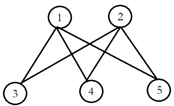
We are given five agents, all are LTI with the TF $G(s)=\frac{1}{s+1}$. We wish to find a $\mathcal{G}$, and a collection of homogeneous controllers, such that $(\mathcal{G},\Sigma,\Pi)$ converges to two clusters, one with two agents and one with three agents. The first cluster should be located at $\mathrm{y}=1$, and the second at $\mathrm{y}=0$.

First, according to the Discussion at Subsection III-C, we want to find a graph $\mathcal{G}$, having five vertices, so that vertices $1,2$ are exchangeable, vertices $3,4,5$ are exchangeable. We consider the graph in Figure 2(a). Obviously, vertices $1,2$ are exchangeable, and vertices $3,4,5$ are exchangeable as well (but not with $1$ and $2$). It can be shown that this is the graph having the minimal number of edges possessing this property. We orient the edges from $1,2$ to $3,4,5$.

Now for the controller synthesis procedure. As we know from [24], not all vectors are available as steady-state outputs of a diffusively-coupled network with prescribed agents. This can be fixed by allowing an addition of an (identical) constant exogenous input to all agents [10], and the steady-state equation becomes $\mathrm{w}=k^{-1}(\mathrm{y})+\mathcal{E}\gamma(\mathcal{E}^{T}\mathrm{y})$ [27]. Writing this equation in coordinates, we get two equations, one for vertices in the $1^{\mathrm{st}}$ cluster, having $\mathrm{y}_{i}=0$, and another for vertices in the $2^{\mathrm{nd}}$ cluster, having $\mathrm{y}_{i}=1$. We get:

where $\gamma_{1}$ is the steady-state input-output relation for each copy of the homogeneous controller. We recall that we also need monotonicity, so $\gamma_{1}$ must be monotone. One possible solution to this set of equations is $w=0.6$ and $\gamma_{1}(x)=-1.2+x$, the latter realized by the controller $\mu_{e}=-1.2+\zeta_{e}$. We simulate the closed-loop system with the prescribed agents and synthesized graph and controllers. The output of the system is available in Figure 4. It is evident that our solution indeed solves the cluster synthesis problem.

References

- [1] A. Schnitzler and J. Gross, “Normal and pathological oscillatory communication in the brain,” Nature reviews. Neuroscience, vol. 6, pp. 285–96, 05 2005.
- [2] N. Chopra and M. Spong, Advances in Robot Control, From Everyday Physics to Human-Like Movements, ch. Passivity-based Control of Multi-Agent Systems, pp. 107–134. Springer, 2006.
- [3] L. Scardovi, M. Arcak, and E. D. Sontag, “Synchronization of interconnected systems with applications to biochemical networks: An input-output approach,” IEEE Transactions on Automatic Control, vol. 55, no. 6, pp. 1367–1379, 2010.
- [4] H. Bai, M. Arcak, and J. Wen, Cooperative Control Design: A Systematic, Passivity-Based Approach. Communications and Control Engineering, Springer, 2011.
- [5] M. Arcak, “Passivity as a design tool for group coordination,” IEEE Transactions on Automatic Control, vol. 52, pp. 1380–1390, Aug. 2007.
- [6] A. Pavlov and L. Marconi, “Incremental passivity and output regulation,” Systems & Control Letters, vol. 57, no. 5, pp. 400 – 409, 2008.
- [7] G. Stan and R. Sepulchre, “Analysis of interconnected oscillators by dissipativity theory,” IEEE Transactions on Automatic Control, vol. 52, pp. 256–270, Feb 2007.
- [8] G. H. Hines, M. Arcak, and A. K. Packarda, “Equilibrium-independent passivity: A new definition and numerical certification,” Automatica, vol. 47, no. 9, pp. 1949–1956, 2011.
- [9] M. Bürger, D. Zelazo, and F. Allgöwer, “Duality and network theory in passivity-based cooperative control,” Automatica, vol. 50, no. 8, pp. 2051–2061, 2014.
- [10] M. Sharf and D. Zelazo, “Analysis and synthesis of mimo multi-agent systems using network optimization,” IEEE Transactions on Automatic Control, 2018.
- [11] L. Xiao and S. Boyd, “Fast linear iterations for distributed averaging,” Systems & Control Letters, vol. 53, no. 1, pp. 65 – 78, 2004.
- [12] L. Stone, R. Olinky, B. Blasius, A. Huppert, and B. Cazelles, “Complex synchronization phenomena in ecological systems,” AIP Conf. Proc., vol. 622, 07 2002.
- [13] K. M. Passino, “Biomimicry of bacterial foraging for distributed optimization and control,” IEEE Control Systems Magazine, vol. 22, pp. 52–67, June 2002.
- [14] C. Altafini, “Consensus problems on networks with antagonistic interactions,” IEEE Transactions on Automatic Control, vol. 58, no. 4, pp. 935–946, 2013.
- [15] J. Qin and C. Yu, “Cluster consensus control of generic linear multi-agent systems under directed topology with acyclic partition,” Automatica, vol. 49, no. 9, pp. 2898 – 2905, 2013.
- [16] Y. Han, W. Lu, and T. Chen, “Cluster consensus in discrete-time networks of multiagents with inter-cluster nonidentical inputs,” IEEE Transactions on Neural Networks and Learning Systems, vol. 24, pp. 566–578, April 2013.
- [17] S. Bonnabel, P. Martin, and P. Rouchon, “Non-linear symmetry-preserving observers on lie groups,” IEEE Transactions on Automatic Control, vol. 54, pp. 1709–1713, July 2009.
- [18] C. Danielson and F. Borrelli, “Symmetric linear model predictive control,” IEEE Transactions on Automatic Control, vol. 60, pp. 1244–1259, May 2015.
- [19] M. W. Spong and F. Bullo, “Controlled symmetries and passive walking,” IEEE Transactions on Automatic Control, vol. 50, pp. 1025–1031, July 2005.
- [20] A. Rahmani and M. Mesbahi, “Pulling the strings on agreement: Anchoring, controllability, and graph automorphisms,” in 2007 American Control Conference, pp. 2738–2743, July 2007.
- [21] A. Chapman and M. Mesbahi, “On symmetry and controllability of multi-agent systems,” in 53rd IEEE Conference on Decision and Control, pp. 625–630, Dec 2014.
- [22] A. Chapman and M. Mesbahi, “State controllability, output controllability and stabilizability of networks: A symmetry perspective,” in 2015 54th IEEE Conference on Decision and Control (CDC), pp. 4776–4781, Dec 2015.
- [23] C. Godsil and G. Royle, Algebraic Graph Theory. Graduate Texts in Mathematics, Springer New York, 2001.
- [24] M. Sharf and D. Zelazo, “A network optimization approach to cooperative control synthesis,” IEEE Control Systems Letters, vol. 1, pp. 86–91, July 2017.
- [25] H. K. Khalil, Nonlinear Systems. Pearson, 3rd ed., 2001.
- [26] R. T. Rockafellar, Convex Analysis. Princeton Landmarks in Mathematics and Physics, Princeton University Press, 1997.
- [27] M. Sharf and D. Zelazo, “Network identification: A passivity and network optimization approach,” in 2018 IEEE 57th Annual Conference on Decision and Control (CDC), 2018.
- [28] R. T. Rockafeller, “Characterization of the subdifferentials of convex functions,” Pacific Journal of Mathematics, vol. 17, no. 3, pp. 497–510, 1966.
- [29] A. Jain, M. Sharf, and D. Zelazo, “Regulatization and feedback passivation in cooperative control of passivity-short systems: A network optimization perspective,” IEEE Control Systems Letters, vol. 2, pp. 731–736, 2018.
- [30] A. Jain, M. Sharf, and D. Zelazo, “Passivation and Cooperative Control of Equilibrium-Independent Passivity-Short Systems,” arXiv e-prints, p. arXiv:1901.06512, 2019.
- [31] A. Cayley, “Desiderata and suggestions: No. 2. the theory of groups: Graphical representation,” American Journal of Mathematics, vol. 1, no. 2, pp. 174–176, 1878.