A simple and efficient architecture for trainable activation functions
Università di Napoli Federico II
Abstract
Learning automatically the best activation function for the task is an active topic in neural network research. At the moment, despite promising results, it is still difficult to determine a method for learning an activation function that is at the same time theoretically simple and easy to implement. Moreover, most of the methods proposed so far introduce new parameters or adopt different learning techniques. In this work we propose a simple method to obtain trained activation function which adds to the neural network local subnetworks with a small amount of neurons. Experiments show that this approach could lead to better result with respect to using a pre-defined activation function, without introducing a large amount of extra parameters that need to be learned.
keywords: neural networks, machine learning, activation functions, adaptive activation functions
1 Introduction
The success of deep learning approaches has led to an increase in interest in MultiLayer FeedForward (MLFF) neural networks. MLFF networks are composed of elementary computing units (neurons), which are organized in layers. The first layer of a MLFF network is composed of input variables. Each neuron belonging to a layer , with , receives possibly connections from all the neurons (or input variables in case of ) of the previous layer . Eeach connection is associated to a real value called weight. The flow of computation proceeds from the first layer to the last layer (forward propagation). The last neuron layer is called output layer, the remaining neuron layers are called hidden layers. The computation of a neuron belonging to the layer corresponds to a two-step process: first is computed the neuron activation and then the neuron output . The neuron activation is usually constructed as a linear combination of the outputs of the previous layer: where is the weight of the connection going to the neuron belonging to the layer to the neuron , is a parameter said , and runs on the indexes of the neurons of the layer which send connections to the neuron . If the the variables correspond to the input variables. The neuron output is usually computed by a differentiable, non linear activation function : . The nonlinear functions are generally chosen as simple fixed functions such as the logistic sigmoid or the tanh function.
Given a MLFF network with input variables and neurons in the output layer, it achieves a functional mapping from a -dimensional space to a -dimensional space. Thus, a MLFF network can be interpreted as a non-linear parametric function , where the parameters are all the weigths and biases of the network and y is the response of the output layer. The approximation properties of MLFF networks have been widely studied (DeVore et al. 1996). In a nutshel, a function approximation problem can be summarized as follows (Bishop 2006; Ripley 2007): given an unknown function and a data set representing a sampling of the unknown function, where , usually called targets, are the values assumed by in with added an unknown noise , the task is to find the appropriate values of the parameters of a parametric function so as to get as close as possible to the unknown function . In this context, there are two different problems, the first one concerns the expressive power of the parameterized function , that is, if there are parameter values for which it is possible to approximate the unknown function , the second one concerns the possibility of actually finding such parameter values. Interestingly, regarding the first problem, a MLFF network with a single hidden layer, which is usually called shallow network, can approximate arbitrarily well any functional continuous mapping defined on a compact input domain, provided the number of hidden neurons is sufficiently large and the activation functions of the hidden neurons satisfy suitable properties, for example, to be sigmoidal or, more in general, not-polynomial functions (Sonoda and Murata 2017; Bishop 2006; Pinkus 1999). In other words, given a certain desired degree of approximation, it exists a set of parameters for which the neural network approaches the unknown function within this degree of approximation, supposed to have a sufficient number of hidden neurons and appropriate activation functions. In this sense, MLFF networks are said to be universal approximators.
However, the key problem is how to find these suitable network parameters, i.e., weights and biases. The process to determine the values of weights and biases on the basis of the data set is called learning or training. Importantly, although the choice of the non linear activation functions does not affect the MLFF network’s universal approximator property, provided certain constraints are satisfied, this choice becomes a key aspect when network weights and biases are to be found during the training process. To clarify this aspect, let us briefly summarize what is a training process. The training process generally corresponds to the minimization of an error function with respect to the network parameters. The error function typically assumes the following form (although many other forms are possible (Bishop 2006) ): where represents the output of the neuron belonging to the output layer as a function of both the input and the network parameters . The quantity represents the target value for output neuron when the input is .The solution for the network parameter values at the global minimum of the error function is usually found by iterating a gradient-based algorithm with the gradient computed through backpropagation (Bishop 2006). Since for MLFF networks the error function typically will be a highly non-linear function of the parameters (not-convex surface), there may exist many local minima or saddlepoints. Notice that parameter regions where the error function is very “flat” can mimick local minima insofar as the learning process is ”trapped” for very long periods of time. In a learning process the main difficult is to avoid these stationary points or regions of the error function. Thus, the choice of the activation functions has a relevant impact on the shape of the error function and, consequently, on the performance of the learning process. Moreover, this choice can affect the number of hidden neurons and layers necessary to reach the desired degree of approximation (Guliyev and Ismailov 2016; Eldan and Shamir 2016).
For these reasons, recently, there is a very large literature proposing activation functions that differ from those standards such as sigmoid and tanh. In particular, the introduction of activation functions as ReLU (Nair and Hinton 2010) and similar functions, such as Leaky ReLU and parametric ReLU described respectively in (Maas et al. 2013) and (He et al. 2015), has contributed to renew the interest of the scientific community for MLFF networks. The use of these new activation functions has been shown to improve significantly the networks in terms of performance and training speed, thanks to properties as no saturation, e.g. (Glorot and Bengio 2010). Another great improvement was given in (Clevert et al. 2015), where the learning is speeded up introducing the ELU activation function, and more recently in (Klambauer et al. 2017) with the introduction of SELU units.
Thus, finding alternative functions that can potentially improve further the results is still an open field of research. Consistent with this perspective, a number of recent papers compare neural architectures with different activation functions, as in (Pedamonti 2018), or propose to search appropriate activation functions within a finite set of potentially interesting activation functions, as in (Ramachandran et al. 2018). However, a very recent field of research focuses on the possibility to learn appropriate activation functions from data, in this way one has adaptable (or trainable) activation functions which are adjusted during the learning phase towards specific functions, allowing the network to exploit the data better (see, for example, (Qian et al. 2018)). Furthermore, any layer of the network could potentially have their own best activation function, increasing the number of choices to make at the design stage. On the other side, it is not guaranteed that fixing the same function for each layer is the best choice. Thus, a way to tackle the problem is to learn the activation functions from data, together with the other parameters of the network; the idea is to find the good activation functions that, together with the other network parameters, provides a good model for the data.
In this paper we introduce a new method for learning activation functions in the context of full-connected and convolutional MLFF neural networks. The impact of this method on the performance of the network are experimentally assessed. The idea is built upon the possibility to obtain adaptable activation functions in terms of sub-networks with just one hidden layer. In a nutshell, each neuron with a non-linear activation function can be substituted with a neuron with an Identity activation function which sends its output to a one-hidden layer sub-network with just one output neuron. This substitution enables us to obtain “any” activation function , since an one-hidden layer neural network can approximate arbitrarily well any functional continuous mapping from one finite-dimensional space to another, provided the number of hidden neurons is sufficiently large and the activation functions of the hidden neurons satisfy suitable properties, for example, to be sigmoidal or, more in general, not-polynomial functions (Sonoda and Murata 2017; Bishop 2006; Pinkus 1999). Thus, our neural network architecture with variable activation functions is again a MLFF neural network. Importantly, this property means that any classical approach applicable to MLFF networks can also be directly applied to our architecture with trainable activation functions. Notably, as we will discuss in Section 2 and 3 our architecture represents a general framework in which several approaches recently proposed in literature can be included.
2 Related work
Over the last years, ReLU has become the standard activation function for deep neural models, surpassing classic functions as sigmoid and tanh used in the past literature thanks to useful properties, such as the ability to avoid saturation issues(Nair and Hinton 2010; Glorot et al. 2011). Different variations of the ReLU have been proposed (Maas et al. 2013; Memisevic et al. 2014; Dugas et al. 2000). All these functions are somehow different from ReLU, but once chosen they remain fixed, with the choice of which one to use taken during the design stage, typically in a heuristic way. A partial attempt to overcome this drawback moves in the direction of searching the best activation function from a predefined set (Liu and Yao 1996; Yao 1999; Ramachandran et al. 2018). These techniques are limited by the fact that the functions are not learned, but just selected from a collection of standard functions. Thus, approaches by trainable activation functions propose more general frameworks. In this direction one can isolate three basic types of approaches: parameterized standard activation function, linear combination of one-variable functions and ensemble of standard activation functions. In Subsection 2.1, 2.2 and 2.3 we will discuss these three types of approaches. In Subsection 2.4 we will present other types of solutions. Our discussion will be mainly based on three dimensions: 1) how many new parameters are added to the network model, 2) the possibility or not to use standard techniques, within neural network context, for learning the new parameters, such as backpropagation for computing the error function gradient or sparse methods, 3) the expressive power of the trainable activation functions.
2.1 Parameterized standard activation functions
With the expression parameterized standard activation functions we refer to all the functions with a shape that is very similar to a given standard activation function, but whose diversity from the latter comes from a set of trainable parameters. The addition of these parameters therefore requires changes, even minimal ones, in the learning algorithm, for example, in the case of using gradient-based methods with backpropagation, the partial derivatives of the error function respect to these new parameters are needed. A first attempt to have a parameterized activation function is given in (Hu 1992) where the proposed activation function uses two trainable parameters to rule the function shape of a classic sigmoidal function. Similar works on sigmoidal and hyperbolic tangent functions are discussed in (Yamada and Yabuta 1992a; Yamada and Yabuta 1992b; Chen and Chang 1996; Singh and Chandra 2003; Chandra and Singh 2004). More recently, the authors in (He et al. 2015) introduce PReLU, a parametric version of ReLU, which modifies the function shape when the argument is negative. However, the resulting function remains basically a modified version of the ReLU function that can change its shape in a restricted domain. In (Clevert et al. 2015) ELU function is proposed, which outperforms the results obtained by ReLU on CIFAR100 dataset, becoming one of the best activation function currently known. However, it needs an external parameter to be set. In (Trottier et al. 2017) PELU unit is proposed, where the need to manually set the parameter is eliminated using two additional trainable parameters.
In all the approaches previously described, although the number of added parameters for each node is low, the expressive power of the trainable activation functions is limited.
2.2 Linear combination of one-variable functions
In this case, activation functions are modelled in terms of linear combinations of one-variable functions. These one-variable functions can in turn have additional parameters. For example, in (Agostinelli et al. 2014) each activation function is represented as a linear combination of hinge-shaped functions. Each hinge-shaped function has just one parameter which regulates the location of the hinge. The number of additional parameters that must be learned when using this approach is , where is the total number of hidden units in the neural network. During the learning phase, the network can be trained using standard methods based on backpropagation. Any continuous piecewise-linear function can be approximated arbitrarily well provided the number of hinge-shaped functions is sufficiently large.
A similar approach has been recently proposed by (Scardapane et al. 2018). In this case, the activation function is modelled as a linear combination of fixed functions, where the fixed functions are defined in terms of parametric kernel functions. The parameters of the kernel functions are computed before the network learning phase by some heuristic procedure applied on the data set. During the network learning phase the number of additional parameters is , however for the kernel functions a number of parameters must be computed in a prior stage (where is the number of parameters of the kernel functions). In case of a correct choice of the parameters of the kernel functions, any continuous one-to-one function defined on a compact set can be approximated arbitrarily well, provided the number of kernel functions is sufficiently large.
In (Ertuğrul 2018), in the context of random weight artificial neural networks, a trainable activation function is proposed in terms of a polynomial function of degree . The coefficients of the polynomial function are computed by linear regression. The number of added parameters corresponds to the number of coefficients for each neuron.
2.3 Ensemble of standard activation functions
In this type of approaches, activation functions are defined as an ensemble of a predetermined number of standard activation functions. For example, the authors of (Jin et al. 2016) designed an activation -shape function composed by three linear functions taking inspiration by Webner-Fechner (Fechner 1966) and Stevens law (Stevens 1957), or in (Qian et al. 2018) a mixture of eLU and ReLU is presented. Interestingly, in (Sütfeld et al. 2018) the authors propose a trainable activation function in terms of a linear combination of different, predefined and fixed functions such as hyperbolic tangent (tanh), ReLU and ELU. The added parameters are the coefficients of the linear combination for each hidden neuron. A similar approach is proposed in (Harmon and Klabjan 2017) where the authors model the trainable activation function as a linear combination of a predefined set of normalized fixed activation functions. The added parameters are the coefficients of the linear combination and a set of offset parameters, and , which are used to dynamically offset the normalization range for each predefined function. Moreover, in order to force the network to choose amongst the predefined activation functions, during the learning process it is required than all the coefficients of the linear combination add to one. This then gives rise to another optimization process unrelated to the classic learning procedure for neural networks
2.4 Other approaches
Two interesting and successful approaches are Maxout(Goodfellow et al. 2013; Sun et al. 2018) and NIN(Lin et al. 2013). However, despite the good performances, both approaches move away from the concept of trainable activation function as it has been previously discussed insofar as the adaptable function does not correspond to the neuron activation function by which the neuron output is computed on the basis of a scalar value (the neuron input) according to the standard two-stage process. In fact, in Maxout, instead of computing the input of a neuron and then assigning it as input to a trainable activation function, input are computed, with , by trainable linear functions, and then the maximum is taken over the output of these linear functions. NIN instead represents an approach used specifically in the case of convolutional neural networks, wherein the nonlinear parts of the filters are replaced with a fully connected neural network acting on all channels simultaneously.
Another interesting way to tackle the problem is to use interpolating functions as in (Scardapane et al. 2017; Trentin 2001). For example, in (Scardapane et al. 2017) the authors propose an adaptable activation function by using a cubic spline interpolation, whose control points for each neuron are adapted in the optimization phase. External methods to classic approaches in neural networks are needed to train the added parameters , where is the number of hidden neurons.
2.5 Summarizing
In all the known approaches, to the best of the our knowledge, either the expressive power of the trainable activation functions is limited or they add new learning mechanisms, constraints and categories of parameters, by contrast in our approach we achieve a feed-forward neural network with trainable activation functions by a feed-forward neural network with fixed activation functions, thus leaving unaltered the classic learning mechanisms and categories of parameters. Thus, in our approach a number of attractive properties are simultaneously satisfied: p1) the trainable activation function can approximate arbitrarily well any continuous one-to-one mapping defined on a compact input domain, p2) any standard learning mechanism for neural network can be directly and easily applied, p3) no learning process in addition to those classically used for neural networks is added, p4) the added parameters are network weights or biases , therefore any classical regularization method can be used, including the possibility of imposing sparsity by using norms such as .
None of the known approaches possess all these properties simultaneously. For example, property p1 is non satisfied for all the approaches discussed in Section 2.1 and 2.3, the approaches discusses in Section 2.2 either do no satisfy property p1 as in (Agostinelli et al. 2014) or property p3 as in (Scardapane et al. 2018).
Interestingly, as we will discuss in Section 3 our architecture represents a general framework in which all the approaches described in Section 2.2 and some of the approaches in Section 2.3 can be included, insofar as any linear combination of one-variable functions can be represented by a sub-network with hidden neurons.
3 System architecture
3.1 Proposed model: Variable Activation Function Subnetwork
In general, as already introduced in Section 1, in a MLFF network the output of a neuron belonging to the -th layer is obtained by a two-step computation (see (Bishop 2006), Chapter 4). The first step computes the input , where runs over neuron’s indexes (or network input values) of the previous layer , which send connections to , are the output of the neurons belonging to the previous layer (or network input values), are the connection weights going from the neurons of the previous layer to the neuron , and is the bias associated to the neuron . The output of the neuron is then computed in a second step transforming the input using a fixed activation function , obtaining .
The key idea of our approach is to implement the second step of the computation by a “small” one-hidden layer sub-network, with hidden neurons and just one input and one output neuron. Let us call it Variable Activation Function (henceforth, VAF) sub-network. So, a VAF for a neuron can be described as a network composed by:
- •
an hidden layer, composed by neurons directly connected to the neuron by a set of weights , with ;
- •
a fixed activation function for the hidden neurons;
- •
an output layer composed by a single neuron connected to all the neurons of the hidden layer by a set of weights , with .
The computation of a VAF sub-network associated to a neuron can be described as follows: VAF sub-network is fed with the input of the neuron , then the neurons of the hidden layer compute outputs as with , while the output neuron computes . and are weights and biases of the hidden layer of the VAF sub-network, respectively, and and are weights and bias of the output layer of VAF sub-network, respectively. In this way the output of the neuron can be expressed as:
| (1) |
, , and are the parameters to be learned from data during the training process.
A general schema of a VAF unit is shown in figure 1. This schema enables one to approximate arbitrarily well any activation function provided that:
- •
the number of hidden neurons in the VAF is sufficiently large;
- •
the activation function of the hidden layer is a not-polynomial function.
As already discussed in Section 1, the first condition is given in (Hornik et al. 1989; Hornik 1991), where it was shown that a shallow networks can approximate any continuous function provided that a sufficient number of hidden neurons are available and that the activation function is continuous, bounded and non-constant. This result was generalized in (Leshno et al. 1993), where it is proved that a shallow network can approximate any continuous function to any degree of accuracy if and only if the network’s activation function is not polynomial. Therefore a VAF activation function can substitute any other network activation function without loss in generality, and having as overhead only an increase in the number of networks parameters, that is equal to with total number of the hidden neurons of the network. Anyway, the number of required parameters can drop to , with number of hidden layers, if we adopt the shared weights principle, so that the functions on the same layer share the same VAF weights. With this design choice, we reduce the number of parameters by making the reasonable assumption that if one function is good for a single neuron, then it should also be good for the other neurons of the same layer. This assumption can also be motivated, instead of under the profile of the sub-networks weights, in terms of activation function of a classic neural networks used in the neural network literature, where neurons on to same layer exhibit the same activation function. Summing up, under the shared weights principle for every network layer the only added hyper-parameters to set are:
- •
the number of hidden neurons of the VAF subnetwork;
- •
the activation function of the VAF hidden neurons.
It is worth to emphasize the fact that, in our approach, we have a neural network architecture which is still a MLFF network with fixed activation functions, without adding any external structure or parameters. Let us clarify this aspect (see also Figure 2). Given a neuron belonging to -th layer of a MLFF network , its output is computed as , in our approach we substitute the activation function with the Identity function, thus obtaining . Then, we add a VAF sub-network which receives as input variable the output of the neuron and computes its output as defined in eq. 1. Finally, this output is sent as input of the next layer of . This procedure is uniformly performed for all the neurons of the MLFF network , but the output layer. Thus, one obtains a new neural network which is still a MLFF network with fixed activation functions, however it behaviours as equipped with trainable activation functions expressed in terms of eq. 1. Consequently, any standard training procedure can be left unaltered (e.g., Stochastic Gradient Descent).
Figure 2 shows how a VAF network can be integrated into a common multilayer full-connected neural network (on the left) and in a convolutional neural network (on the right).
Notably, given that a VAF subnetwok performs a linear combination of one-variable functions, any approach discussed in Section 2.2 can be included in this schema, provided to choose suitably the activation function and the parameters and .
3.2 VAF network learning
As discussed above, our neural architecture including VAF is a MLFF network, consequently it can be trained using any learning algorithm dedicated to MLFF network. However, in case of the same VAF acting uniformly for all neurons of a layer, then there is the constrain that the weights of VAF networks should be considered shared weights. From an implementation point of view this corresponds to consider a VAF network as a function convolving with the values (Lin et al. 2013). The weight values of the VAF, being few and connected to each unit, influence the behaviour of the entire network, therefore their behaviour must be taken into consideration during the training phase, and, in particular, the initial value of the VAF weights can be decisive. The training of a neural network usually starts initializing the weights and biases in a random way (Bishop 2006), or using any initialization rule as for example (Glorot and Bengio 2010). Although these approaches can also be followed in our case, it is possible to choose different solutions for the VAF weights initialization. In particular, a possible alternative is to select the initial weights of the VAF so that at the beginning of the learning process the VAF networks approximate a fixed function. For example, we can select a classic activation function as ReLU or sigmoid, or the activation function associated to the other hidden layers of the network. In this way hypothetically the function would start from a notoriously already valid form in which the training process should only modify it just enough to improve the performance of the network based on the training data. However, it should be kept in mind that this choice can affect negatively the solution generated by the learning process, given that the resulting VAF can be too similar to the initial function.
4 Experimental results
In this section we provide an experimental evaluation of the proposed trainable activation function architecture. In order to achieve a first clue on the validity of our approach, and some heuristic indications for the initialization strategies of VAF networks, in Section 4.1 we report some preliminary experiments on Sensorless, a relatively small classification dataset used as standard benchmark for supervised techniques.
On the basis of the results of these experiments, we performed two different series of experiments to test our approach on MLFF networks. In the former, we consider standard MLFF networks (Section 4.2) , and in the latter convolutional MLFF networks (Section 4.3). In Section 4.2 we consider both classification and regression problems using different datasets. In Section 4.3 we consider more large-scale dataset as MNIST, Fashion MNIST and CIFAR10.
4.1 VAF subnetworks: Activation functions, number of hidden neurons and weight initialization
For a preliminary analysis of the validity of our approach, and for defining some heuristic choices about VAF subnets such as the number and the activation functions of the hidden neurons, we perform a series of experiments on Sensorless dataset (see table 1 for details), partitioning it in a random sample of 60% for training, 20% for validation and another 20% for testing. According to what was also reported in (Scardapane et al. 2018), if one uses a standard shallow network, i.e., -hidden layer network, we found that tanh is the best fixed activation function for this dataset. In particular, using a shallow network with hidden neurons we obtained an accuracy on the test set very close to 100%. Thus, to better investigate the impact of our approach we chose a more “difficult situation” for a shallow network using network models with a small number of hidden neurons. More in detail, we selected three small shallow nets with , and hidden neurons.
For each model, We perform a set of experiments using different activation functions.
Firstly, we train these small networks using as fixed activation functions either or , then we repeat the same experiments substituting the fixed activation functions with VAF subnets as described in Section 3. We considered several scenarios: 1) different number of VAF hidden neurons, in particular ; 2) tanh and ReLU as activation functions for VAF hidden neurons; 3) two different strategies for weight initialization of VAF subnets, both a classic random initialization and a weight initialization by which VAF subnets have a behaviour very similar to activation functions of the VAF hidden neurons, we will call the latter specific weight initialization; 4) as discussed in Section 3, we examine both the case in which VAF subnets on the same layer share the weights (shared weights principle) and the case in which VAF subnets on the same layer can have different weights.
We trained all the networks using ADAM algorithm (Kingma and Ba 2014) for epochs. Furthermore, we repeat our experiments for times.
Results
In Figure 3(a), 3(b) and 3(c) are reported the results with respect to the shallow networks with , and hidden neurons, respectively, in the case in which VAF subnets on the same layer do not share the weights. In Figure 4(a), 4(b) and 4(c) are reported the results in the case in which VAF subnets on the same layer share the weights.


Notably, one can observe that all the models equipped with VAF subnets outperform the corresponding shallow networks. Interestingly, these results support the possibility of using a shared VAF approach with a fairly low number of VAF hidden neurons, thus having a lower number of parameters to be learned. In fact, the two approaches, non-shared (Figure 3) and shared (Figure 4) VAF subnets, exhibit a very similar behaviour, and although in all cases accuracy tends to increase as the number of neurons of the VAF subnets increases, this increase is not always very relevant. The two types of VAF weight initialization seem to give similar results, with slightly better performances for random initialization. The use of tanh or ReLU as activation function of VAF hidden neurons, on the other hand, seems to significantly change the network performance. In fact, the accuracy obtained by networks with ReLU activation function for the VAF hidden neurons is uniformly lower than those obtained with the tanh activation function. We suppose that this result is due to the fact that we are always using shallow nets.
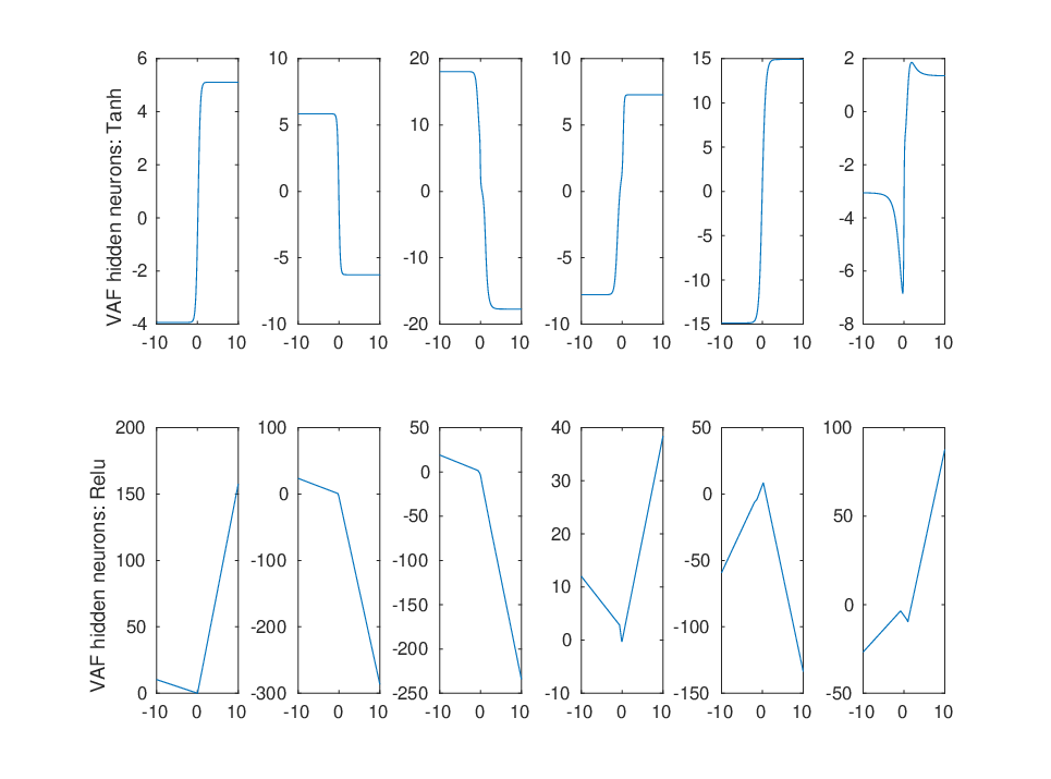
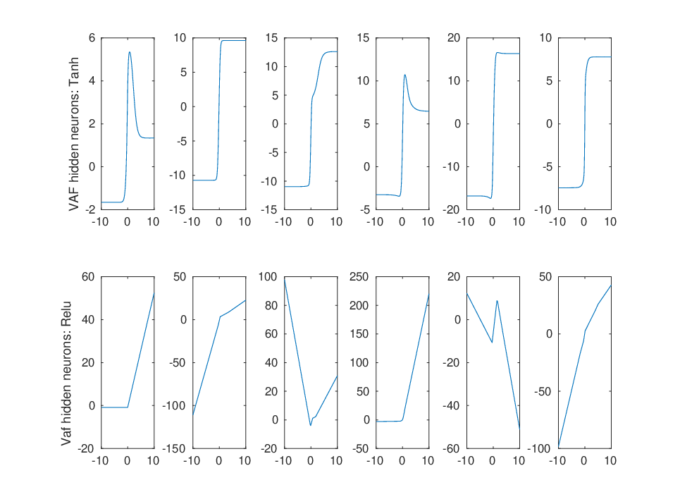
In Figure 5(a) and 5(b) are reported the output values of trained VAF subnetworks when a random or a specific weight initialization is chosen, respectively. One can note that the resulting activation functions are often strongly different from the classic tanh and ReLU, and that they exhibit similarly a high degree of non-linearity.
4.2 Full-connected MLFF networks: classification and regression
In this experimental scenario we focus on evaluating the impact of both VAF subnetworks and VAF weight initialization using full-connected MLFF networks with or hidden layers trained on public datasets (see Table 1). of these datasets are suitable for classification problems, and for regression problems. The number of hidden neurons varies in the set , but for neural networks with hidden layers we only selected neural networks with a number of hidden neurons belonging to the first layer larger than the number of hidden neurons of the second layer. ReLU was selected as activation function of the hidden neurons of VAF sub-networks. Thus, for each dataset we obtained network models with -hidden layer, and with -hidden layers. Let us call and the -hidden and -hidden layer networks, respectively, with . On the basis of what was discussed in Section 3, to each network () it is possible to associate a neural network () equipped with VAF subnetworks, where is the number of hidden neurons of VAF subnetworks.
On the basis of the results discussed in Section 4.1, we considered VAF subnets shared on each layer, and . In Table 2 we report the neural network architectures used in this series of experiments. Neural network architectures were sorted in ascending order according to their complexity. Networks were trained according to an usual learning approach, described in Algorithm 1. In particular, we used a batch approach, RProp (Riedmiller and Braun 1992), with “small” datasets, i.e, when the number of examples was less than , otherwise we used a mini-batch approach, RMSProp (Tieleman and Hinton 2012). Moreover, networks with VAF subnetworks were trained using both a random initialization and an specific weight initialization such that they approximate a ReLU function. All the network models, i.e., ,, and were compared in a -fold cross validation schema (see Algorithm 2), with .
Note that Learning Rate (LR) in RMSProp spans in the range , considering equispaced values, while in RProp was selected equal to , and equal to . In Table 3 are summarized the parameters of this series of empirical evaluations.
| Name | Istances | Input Dim. | N. classes | Task | Neural Network Arch. | Ref. |
| CPU-Small | 8192 | 12 | - | Regress. | MLFF | Dheeru and Karra Taniskidou 2017 |
| DeltaElevator | 9517 | 6 | - | Regress. | MLFF | https://www.dcc.fc.up.pt 2009 |
| Elevators | 16599 | 18 | - | Regress. | MLFF | https://www.dcc.fc.up.pt 2009 |
| Kinematics | 8192 | 8 | - | Regress. | MLFF | https://www.dcc.fc.up.pt 2009 |
| Puma-8NH | 8192 | 8 | - | Regress. | MLFF | https://www.dcc.fc.up.pt 2009 |
| Puma-32NH | 8192 | 32 | - | Regress. | MLFF | https://www.dcc.fc.up.pt 2009 |
| Servo | 197 | 4 | - | Regress. | MLFF | Dheeru and Karra Taniskidou 2017 |
| Energy Cooling | 768 | 8 | - | Regress. | MLFF | https://www.dcc.fc.up.pt 2009 |
| Energy Heating | 768 | 8 | - | Regress. | MLFF | https://www.dcc.fc.up.pt 2009 |
| Yatch | 308 | 7 | - | Regress. | MLFF | Dheeru and Karra Taniskidou 2017 |
| Sensorless | 11 | Classif | MLFF | Dheeru and Karra Taniskidou 2017 | ||
| Liver | Classif. | MLFF | Dheeru and Karra Taniskidou 2017 | |||
| Wine | Classif. | MLFF | Dheeru and Karra Taniskidou 2017 | |||
| Statlog Image Segmentation | Classif. | MLFF | Dheeru and Karra Taniskidou 2017 | |||
| Statlog Landsat Satellite | Classif. | MLFF | Dheeru and Karra Taniskidou 2017 | |||
| Cardiotocography | Classif. | MLFF | Dheeru and Karra Taniskidou 2017 | |||
| Seismic bumps | Classif. | MLFF | Sikora and Wróbel 2010 | |||
| Dermatology | Classif. | MLFF | Dheeru and Karra Taniskidou 2017 | |||
| Diabetic retinopathy debrecen | Classif. | MLFF | Antal and Hajdu 2014 | |||
| QSAR biodegradation | Classif. | MLFF | Mansouri et al. 2013 | |||
| Climate model simulation | Classif. | MLFF | Lucas et al. 2013 | |||
| MNIST | Classif. | CNN | LeCun and Cortes 2010 | |||
| Fashion MNIST | Classif. | CNN | Xiao et al. 2017 | |||
| Cifar10 | Classif. | CNN | Krizhevsky and Hinton 2009 |
| #1 | #2 | #3 | #4 | #5 | #6 | #7 | #8 | #9 | #10 | |
|---|---|---|---|---|---|---|---|---|---|---|
| Stand | ||||||||||
| VAF |
| , | k | VAF initialization | Learning approaches | # maximum epochs | K |
|---|---|---|---|---|---|
| {10, 25, 50, 100} | {3} | {Random, ReLU} | {RMSProp, RProp} | 300 | 10 |
Results
In Table 4 and 5 are showed mean and standard deviations of RMSE and accuracy for regression and classification datasets, respectively, by using a K-fold cross-validation approach. The best results are displayed in bold.
In case of the regression datasets, VAF approach uniformly overcomes standard approach. Only in one case we obtain the best result with a standard approach. For four datasets (DeltaElevator, Elevators, Puma-32H and Yatch) RMSE ’s mean obtained by VAF networks results much smaller than RMSE obtained by neural network without VAF subnetwork. For example in DeltaElevator dataset RMSE’s mean was reduced by two (VAF init random) and one (VAF Init ReLU) order of magnitude. Moreover standard deviations remain comparable or lower than those without VAF subnetworks. This suggests that the training process of network with VAF subnetworks is sufficiently stable.
Similar results were obtained with classification datasets (see Table 5). Neural networks with VAF outperforms neural networks without VAF. Only in two datasets () neural networks without VAF outperforms neural networks with VAF. Also in this case, standard deviations remain comparable or lower than those without VAF.
| standard Relu | VAF Init random | VAF Init ReLU | ||
|---|---|---|---|---|
| RMSE: mean + St.Dev | RMSE: mean + St.Dev | RMSE: mean + St.Dev | ||
| CPUsmall | () | () | () | |
| DeltaElevator | () | () | () | |
| Elevators | () | () | () | |
| Kinematics | () | () | () | |
| Puma-8NH | () | () | () | |
| Puma-32H | () | () | () | |
| Servo | () | () | () | |
| Energy Cooling | () | () | () | |
| Energy Heating | () | () | () | |
| Yatch | () | () | () |
| standard Relu | VAF Init random | VAF Init ReLU | ||
|---|---|---|---|---|
| Accuracy: mean + St.Dev | Accuracy: mean + St.Dev | Accuracy: mean + St.Dev | ||
| Liver | () | () | () | |
| Wine | () | () | () | |
| Image segmentation | () | () | () | |
| Satellite image | () | () | () | |
| CTG | () | () | () | |
| Seismic bumps | () | () | () | |
| Dermatology | () | () | () | |
| Diabetic | () | () | () | |
| Biodegradation | () | () | () | |
| Climate simulation | () | () | () |
4.3 Convolutional MLFF networks
In order to evaluate experimentally the impact of VAF on Convolutional Neural Networks (CNN), we consider standard CNN networks with and convolutional layers, and run experiments on three different dataset: MNIST, Fashion MNIST and CIFAR10 (see Table 1 for further details). As discussed in Section 3.2 and Section 4.2, a key aspect is the initialization of the VAF networks. Thus, also in this case, we chose to initialize the weights of the VAF subnetworks either randomly or to approximate a ReLU function. To this aim, we build two CNN architectures (similar to the basic network used in (Lin et al. 2013)), the first one composed of -layer CNN networks used for MNIST and Fashion-MNIST and the second one composed of -layers trained and tested with the more complex CIFAR10 dataset. Let us call and respectively the -layer CNN and the -layer CNN; as stated in Section 3, it is possible to associate to each a neural network equipped with VAF sub-networks having hidden units. The experiments were preformed using a -fold cross validation schema as described in 2. Networks were trained using Stochastic Gradient Descent (SGD) method with mini-batching.
Furthermore, we compare our architecture with two other neural architectures also equipped with trainable activation functions. The first one is KAFnet, a very recent and promising approach proposed in (Scardapane et al. 2018) and already discussed in Section 2.2. The second one is Network in Network (NIN), a successful approach proposed in (Lin et al. 2013) and already discussed in Section 2.4. To this aim, we used the same experimental settings described in (Scardapane et al. 2018), i.e., a convolutional MLFF network composed by two convolutional layers, each of these followed by a maxpooling layer and a dropout layer of (see Table 6). To distinguish it from the others models, we will call this network . Starting from , we obtained three different types of neural networks with trainable activation functions according to three different procedures proposed for KAFnet, NIN and VAF. We use the classic CIFAR10 data configuration ( training samples + test samples) to train the three types of obtained networks. The network with fixed activation function corresponding to ReLU is also considered as baseline. Finally, we repeat the same setup using MNIST and Fashion-MNIST dataset.
Properties of the used CNN architectures and learning process are summarised in table 6.
| Name | Layers | VAF initialization | Learning approaches | # maximum epochs |
|---|---|---|---|---|
| (Conv. + Maxout + Dropout) | {Random, ReLU} | SGD | 300 | |
| (Conv. + Maxout + Dropout) | {Random, ReLU} | SGD | 300 | |
| (Conv. + Maxout + Dropout) | Random | Adam | 300 |
Results
In Table 7 are shown mean and standard deviations of accuracies for the three datasets Cifar10, MNIST and Fashion MNIST, using a -fold cross-validation approach for the neural architecture summarized in the first two rows of Table 6.
The best results are reported in bold style. One can note that VAF approach uniformly outperforms the standard approach, especially when using a random initialization scheme.
Also in this experimental scenario the standard deviations obtained by networks with VAF remain comparable or lower than those without VAF subnetworks.
Especially for the CIFAR10 dataset, we obtain a considerable improvement.
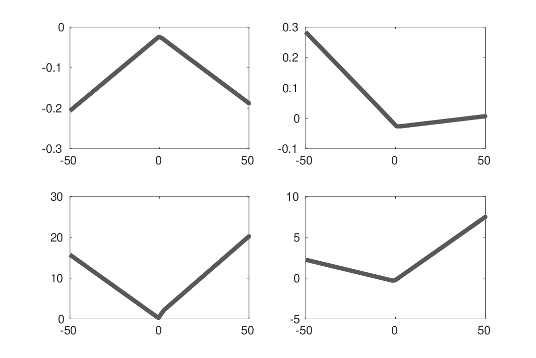
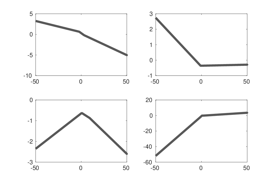
In Figures 7 and 8 are shown some examples of trained activation functions respectively in and ; it should be noted the influence of VAF initialization on the trained activation function: it seems that, in case of initialization as ReLU, the initial shape remains mostly unchanged, giving a resulting function that looks like a PReLU/Leaky ReLU. A more interesting behaviour is given by random initialization, where every VAF unit seems to exhibit greater changes respect to the initial function. This greater variability given by random initialization respect to ReLU initialization seems to give an improvement in accuracy results as shown in Table 7.
In Table 8 we show the performances of KAFnet, NIN and VAF network on the two datasets Fashion-MNIST and CIFAR10 6 in terms of accuracy. VAF network outperforms KAF and NIN on both the dataset CIFAR10 and Fashion MNIST. We do not report the MNIST results because are all very similar between them (over the of accuracy). Notably, therefore, also with respect to two other two approaches with trainable activation functions known in literature, our approach results in better performance.
| standard ReLU | VAF Init random | VAF Init ReLU | ||
|---|---|---|---|---|
| Acc. + St.Dev | Acc. + St.Dev | Acc. + St.Dev | ||
| Cifar10 | ||||
| MNIST | ||||
| Fashion MNIST |
| standard ReLU | VAF(M=5) | KAF(D=20) | NIN | |
|---|---|---|---|---|
| Accuracy | Accuracy | Accuracy | Accuracy | |
| Cifar10 | ||||
| MNIST | ||||
| Fashion MNIST |


5 Conclusion
In this work, we proposed a simple and direct way to obtain adaptable activation functions in feed-forward neural networks. In particular, we proposed to modify a feed-forward neural network by adding Variable Activation Functions (VAF) in terms of one-hidden layer subnetworks (see Section 3). The resulting network is still a feed-forward neural network. The proposed architecture doesn’t need many more parameters than networks using not adaptable activation functions as ReLU, and the learning process follows standard approaches (see Section 3.2). Importantly, VAF subnetworks can approximate arbitrarily well any activation functions, provided that the number of hidden neurons is sufficiently large (see Section 3).
It is worth to remark that our approach distinguishes from other approaches proposed in literature insofar as it satisfies simultaneously the properties p1 – p4 as described in Section 2.5. These properties include a high expressive power of the trainable activation functions, no external parameter or learning process in addition to the classical ones for neural networks, and the possibility to use classical regularization methods.
Interestingly, as we discussed in Section 3 our architecture represents a general framework in which all the approaches described in Section 2.2 and some of the approaches in Section 2.3 can be included.
We experimentally evaluated our architecture on three different sets of experiments. In the former (see Section 4.1, we tested our approach using small shallow networks for defining some heuristic choices about VAF subnets. Notably, all the models equipped with VAF subnets outperform the corresponding shallow networks, and the results support the possibility of using a shared VAF approach with a fairly low number of VAF hidden neurons. In the second series of experiments (see Section 4.2), we considered full-connected Multi-Layered Neural Network (MLFF) networks. More specifically, we selected networks with or hidden layers. A correspondent network with VAF subnetworks was built for each of these networks (see Section 3 and 4.2). We obtained a total of different neural network architectures. These neural architectures were evaluated and compared using a -Fold Cross-Validation procedure (see Algorithm 2) on different datasets (see Table 1), either for classification tasks or regression tasks. The results show that the networks with VAF subnetworks are uniformly more performing than the ones without VAF networks. In particular, our approach outperforms that without VAF networks on the of the datasets. Only on three datasets our approach had worse results.
In the last set of experiments, we considered Convolutional Neural Networks with and layers and correspondent networks with VAF units and we evaluate them using image datasets (MNIST, Fashion MNIST and CIFAR10)for classification. Also in this case the VAF subnetworks outperform networks with static units and selected state-of-the-art neural architectures (KAFNet and NIN) equipped with trainable activation functions.
In conclusion, VAF units have been tested using traditional MLNN networks and CNN networks with various datasets and give better results compared with networks with similar design both with traditional ReLU functions and trainable activation functions. We showed that is possible to obtain encouraging results without the need to use complex designs, particular initialization schemes or learning process in addition to those classically used for neural networks.
Acknowledgements
The work has been partially supported by the national project Perception, Performativity and Cognitive Sciences - PRIN2015 Cod. 2015TM24JS_009.
References
- DeVore et al. [1996] Ronald A DeVore, Konstantin I Oskolkov, and Pencho P Petrushev. Approximation by feed-forward neural networks. Annals of Numerical Mathematics, 4:261–288, 1996.
- Bishop [2006] C.M. Bishop. Pattern Recognition and Machine Learning. Springer, 2006.
- Ripley [2007] Brian D Ripley. Pattern recognition and neural networks. Cambridge university press, 2007.
- Sonoda and Murata [2017] Sho Sonoda and Noboru Murata. Neural network with unbounded activation functions is universal approximator. Applied and Computational Harmonic Analysis, 43(2):233–268, 2017.
- Pinkus [1999] Allan Pinkus. Approximation theory of the mlp model in neural networks. Acta Numerica, 8(January):143–195, 1999.
- Guliyev and Ismailov [2016] Namig J Guliyev and Vugar E Ismailov. A single hidden layer feedforward network with only one neuron in the hidden layer can approximate any univariate function. Neural computation, 28(7):1289–1304, 2016.
- Eldan and Shamir [2016] Ronen Eldan and Ohad Shamir. The power of depth for feedforward neural networks. In Conference on Learning Theory, pages 907–940, 2016.
- Nair and Hinton [2010] Vinod Nair and Geoffrey E. Hinton. Rectified linear units improve restricted boltzmann machines. In ICML, pages 807–814, 2010.
- Maas et al. [2013] Andrew L Maas, Awni Y Hannun, and Andrew Y Ng. Rectifier nonlinearities improve neural network acoustic models. In Proc. icml, 2013.
- He et al. [2015] Kaiming He, Xiangyu Zhang, Shaoqing Ren, and Jian Sun. Delving deep into rectifiers: Surpassing human-level performance on imagenet classification. In Proceedings of the IEEE international conference on computer vision, pages 1026–1034, 2015.
- Glorot and Bengio [2010] Xavier Glorot and Yoshua Bengio. Understanding the difficulty of training deep feedforward neural networks. In AISTATS, volume 9, pages 249–256, 2010.
- Clevert et al. [2015] Djork-Arné Clevert, Thomas Unterthiner, and Sepp Hochreiter. Fast and accurate deep network learning by exponential linear units (elus). CoRR, abs/1511.07289, 2015.
- Klambauer et al. [2017] Günter Klambauer, Thomas Unterthiner, Andreas Mayr, and Sepp Hochreiter. Self-normalizing neural networks. CoRR, abs/1706.02515, 2017.
- Pedamonti [2018] Dabal Pedamonti. Comparison of non-linear activation functions for deep neural networks on mnist classification task. CoRR, abs/1804.02763, 2018.
- Ramachandran et al. [2018] Prajit Ramachandran, Barret Zoph, and Quoc V. Le. Searching for activation functions. In 6th International Conference on Learning Representations (ICMR), 2018, 2018.
- Qian et al. [2018] Sheng Qian, Hua Liu, Cheng Liu, Si Wu, and Hau-San Wong. Adaptive activation functions in convolutional neural networks. Neurocomputing, 272:204–212, 2018.
- Glorot et al. [2011] Xavier Glorot, Antoine Bordes, and Yoshua Bengio. Deep sparse rectifier neural networks. In Proceedings of the fourteenth international conference on artificial intelligence and statistics, pages 315–323, 2011.
- Memisevic et al. [2014] Roland Memisevic, Kishore Reddy Konda, and David Krueger. Zero-bias autoencoders and the benefits of co-adapting features. CoRR, abs/1402.3337, 2014.
- Dugas et al. [2000] Charles Dugas, Yoshua Bengio, François Bélisle, Claude Nadeau, and René Garcia. Incorporating second-order functional knowledge for better option pricing. In NIPS, pages 472–478, 2000.
- Liu and Yao [1996] Yong Liu and Xin Yao. Evolutionary design of artificial neural networks with different nodes. In International Conference on Evolutionary Computation, pages 670–675, 1996.
- Yao [1999] X. Yao. Evolving artificial neural networks. Proceedings of the IEEE, 87:1423–1447, 1999.
- Hu [1992] Shao H. Hu, Z. The study of neural network adaptive control systems. Control and Decision, 7(2):361–366, 1992.
- Yamada and Yabuta [1992a] T. Yamada and T. Yabuta. Neural network controller using autotuning method for nonlinear functions. IEEE Transactions on Neural Networks, 3(4):595–601, 1992a.
- Yamada and Yabuta [1992b] T. Yamada and T. Yabuta. Remarks on a neural network controller which uses an auto-tuning method for nonlinear functions. In [Proceedings 1992] IJCNN International Joint Conference on Neural Networks, volume 2, pages 775–780 vol.2, 1992b.
- Chen and Chang [1996] Chyi-Tsong Chen and Wei-Der Chang. A feedforward neural network with function shape autotuning. Neural networks, 9(4):627–641, 1996.
- Singh and Chandra [2003] Yogesh Singh and Pravin Chandra. A class+ 1 sigmoidal activation functions for ffanns. Journal of Economic Dynamics and Control, 28(1):183–187, 2003.
- Chandra and Singh [2004] Pravin Chandra and Yogesh Singh. An activation function adapting training algorithm for sigmoidal feedforward networks. Neurocomputing, 61:429–437, 2004.
- Trottier et al. [2017] Ludovic Trottier, Philippe Gigu, Brahim Chaib-draa, et al. Parametric exponential linear unit for deep convolutional neural networks. In Machine Learning and Applications (ICMLA), 2017 16th IEEE International Conference on, pages 207–214. IEEE, 2017.
- Agostinelli et al. [2014] Forest Agostinelli, Matthew Hoffman, Peter J. Sadowski, and Pierre Baldi. Learning activation functions to improve deep neural networks. CoRR, abs/1412.6830, 2014.
- Scardapane et al. [2018] Simone Scardapane, Steven Van Vaerenbergh, Simone Totaro, and Aurelio Uncini. Kafnets: Kernel-based non-parametric activation functions for neural networks. Neural Networks, 2018.
- Ertuğrul [2018] Ömer Faruk Ertuğrul. A novel type of activation function in artificial neural networks: Trained activation function. Neural Networks, 99:148–157, 2018.
- Jin et al. [2016] Xiaojie Jin, Chunyan Xu, Jiashi Feng, Yunchao Wei, Junjun Xiong, and Shuicheng Yan. Deep learning with s-shaped rectified linear activation units. In Proceedings of the Thirtieth AAAI Conference on Artificial Intelligence, pages 1737–1743. AAAI Press, 2016.
- Fechner [1966] Gustav Fechner. Elements of psychophysics. New York, Holt, Rinehart and Winston, 1966.
- Stevens [1957] Stanley S Stevens. On the psychophysical law. Psychological review, 64(3):153, 1957.
- Sütfeld et al. [2018] Leon René Sütfeld, Flemming Brieger, Holger Finger, Sonja Füllhase, and Gordon Pipa. Adaptive blending units: Trainable activation functions for deep neural networks. arXiv preprint arXiv:1806.10064, 2018.
- Harmon and Klabjan [2017] Mark Harmon and Diego Klabjan. Activation ensembles for deep neural networks. CoRR, abs/1702.07790, 2017.
- Goodfellow et al. [2013] Ian J. Goodfellow, David Warde-Farley, Mehdi Mirza, Aaron Courville, and Yoshua Bengio. Maxout networks. In Proceedings of the 30th International Conference on International Conference on Machine Learning - Volume 28, ICML’13, pages III–1319–III–1327, 2013.
- Sun et al. [2018] Weichen Sun, Fei Su, and Leiquan Wang. Improving deep neural networks with multi-layer maxout networks and a novel initialization method. Neurocomputing, 278:34 – 40, 2018.
- Lin et al. [2013] Min Lin, Qiang Chen, and Shuicheng Yan. Network in network. CoRR, abs/1312.4400, 2013.
- Scardapane et al. [2017] Simone Scardapane, Michele Scarpiniti, Danilo Comminiello, and Aurelio Uncini. Learning activation functions from data using cubic spline interpolation. In Italian Workshop on Neural Nets, pages 73–83. Springer, 2017.
- Trentin [2001] Edmondo Trentin. Networks with trainable amplitude of activation functions. Neural Networks, 14(4-5):471–493, 2001.
- Hornik et al. [1989] Kurt Hornik, Maxwell Stinchcombe, and Halbert White. Multilayer feedforward networks are universal approximators. Neural Networks, 2(5):359 – 366, 1989. ISSN 0893-6080. doi: https://doi.org/10.1016/0893-6080(89)90020-8. URL http://www.sciencedirect.com/science/article/pii/0893608089900208.
- Hornik [1991] Kurt Hornik. Approximation capabilities of multilayer feedforward networks. Neural networks, 4(2):251–257, 1991.
- Leshno et al. [1993] Moshe Leshno, Vladimir Ya Lin, Allan Pinkus, and Shimon Schocken. Multilayer feedforward networks with a nonpolynomial activation function can approximate any function. Neural networks, 6(6):861–867, 1993.
- Kingma and Ba [2014] Diederik Kingma and Jimmy Ba. Adam: A method for stochastic optimization. In International Conference on Learning Representations, 12 2014.
- Riedmiller and Braun [1992] Martin Riedmiller and Heinrich Braun. Rprop - a fast adaptive learning algorithm. Technical report, Proc. of ISCIS VII), Universitat, 1992.
- Tieleman and Hinton [2012] Tijmen Tieleman and Geoffrey Hinton. Lecture 6.5-rmsprop: Divide the gradient by a running average of its recent magnitude. COURSERA: Neural networks for machine learning, 4(2):26–31, 2012.
- Dheeru and Karra Taniskidou [2017] Dua Dheeru and Efi Karra Taniskidou. UCI machine learning repository, 2017.
- https://www.dcc.fc.up.pt [2009] https://www.dcc.fc.up.pt. https://www.dcc.fc.up.pt, June 2009.
- Sikora and Wróbel [2010] Marek Sikora and Łukasz Wróbel. Application of rule induction algorithms for analysis of data collected by seismic hazard monitoring systems in coal mines. Archives of Mining Sciences, 55(1):91–114, 2010.
- Antal and Hajdu [2014] Bálint Antal and András Hajdu. An ensemble-based system for automatic screening of diabetic retinopathy. Knowledge-based systems, 60:20–27, 2014.
- Mansouri et al. [2013] Kamel Mansouri, Tine Ringsted, Davide Ballabio, Roberto Todeschini, and Viviana Consonni. Quantitative structure-activity relationship models for ready biodegradability of chemicals. Journal of Chemical Information and Modeling, 53(4):867–878, 2013.
- Lucas et al. [2013] D. D. Lucas, R. Klein, J. Tannahill, D. Ivanova, S. Brandon, D. Domyancic, and Y. Zhang. Failure analysis of parameter-induced simulation crashes in climate models. Geoscientific Model Development, 6(4):1157–1171, 2013.
- LeCun and Cortes [2010] Yann LeCun and Corinna Cortes. MNIST handwritten digit database. http://yann.lecun.com/exdb/mnist/, 2010. URL http://yann.lecun.com/exdb/mnist/.
- Xiao et al. [2017] Han Xiao, Kashif Rasul, and Roland Vollgraf. Fashion-mnist: a novel image dataset for benchmarking machine learning algorithms. CoRR, abs/1708.07747, 2017.
- Krizhevsky and Hinton [2009] A Krizhevsky and G Hinton. Learning multiple layers of features from tiny images. In Computer Science Department, University of Toronto, Tech. Rep, volume 1, 01 2009.