Amplitudes’ Positivity, Weak Gravity Conjecture, and Modified Gravity

The general properties of the S-matrix, unitarity, analyticity and crossing symmetry, imply dispersion relations for forward elastic scattering amplitudes, which in turn yield positivity bounds for amplitudes evaluated in the infrared (IR). They provide therefore non-trivial constraints on the coefficients of operators in the effective field theories (EFTs) that are used to calculate the amplitudes at low energy Adams:2006sv; Bellazzini:2016xrt. An EFT with operators entering the action with the “wrong” sign cannot arise as the low-energy limit of a consistent ultraviolet (UV) theory satisfying the S-matrix axioms, and thus lives in the “swampland.” The proof of the a-theorem Komargodski:2011vj; Luty:2012ww is perhaps the prime example of an application of these positivity bounds.

In this paper, new amplitudes’ positivities are derived for theories with a massless graviton in the spectrum, despite the fact that the forward elastic 2-to-2 scattering is singular (Coulomb singularity). These new positivity bounds, and the way we circumvent the graviton forward singularity, are extremely important because they allow us to address the swampland program of quantum gravity and modified gravity theories, providing general and robust results.

As a notable application, we study the Einstein-Maxwell theory, i.e. the low-energy EFT of an abelian $U(1)$ gauge theory coupled to gravity, and show that our positivity bounds imply certain inequalities among the leading higher-dimensional operators affecting the black hole’s extremality condition (the minimal mass for which a charged black hole can exist, as opposed to a naked singularity). We show that extremal black holes of mass $M$ and $U(1)$-charge $Q$ must satisfy $\sqrt{2}m_{\mathrm{Pl}}|Q|/M>1$, so that they are self-repulsive and are no longer kinematically forbidden from decaying into smaller extremal black holes. Moreover, these positivity bounds provide a proof of the mild form of the weak gravity conjecture (WGC) ArkaniHamed:2006dz: extremal black holes are themselves charged states in the theory for which gravity is the weakest force.

Another interesting application is for shift-symmetric scalars such as in the EFT of axions, $P(X)$ theories, and weakly broken galileons. The latter are found to have a tiny cutoff if they are to originate from a canonical microscopic S-matrix, $\Lambda_{UV}<\mathrm{few}\times(H^{3}m_{\mathrm{Pl}})^{1/4}\sim 1/(10^{7}\mathrm{km})$, i.e. orders of magnitude smaller than the strong coupling scale $\Lambda_{3}=(H^{2}m_{\mathrm{Pl}})^{1/3}\sim 1/(10^{3}\text{ km})$.

Finally, we also discuss how our methods allow us to derive positivity bounds in a mildly curved de Sitter (dS) spacetime.

The forward elastic amplitude of massless particles of polarizations labelled by $z_{i}$ is dominated by the universal Coulomb singularity

$$\mathcal{M}^{z_{1}z_{2}}(s,t\rightarrow 0)=-\frac{s^{2}}{m_{\mathrm{Pl}}^{2}t}+O(s)\,,$$

(1)

because of the equivalence principle or, equivalently, because of factorization of the amplitude at the pole into the soft emission of an on-shell massless graviton, which has universal strength given by the reduced Planck mass $m_{\mathrm{Pl}}$. Since the coefficient of $s^{2}$ in (1) would enter the dispersion relation in the forward limit for particles of any spin $z_{i}$ Bellazzini:2016xrt, see (4), the naïve application of the Cauchy integral theorem to $\mathcal{M}^{z_{1}z_{2}}(s,t\rightarrow 0)$ yields $\infty=\infty$, which is consistent, but admittedly not very informative. It is clear, however, that this divergence is due to long-distance physics, i.e. vanishing exchanged momentum, corresponding to the graviton probing arbitrarily large macroscopic distances even for large center-of-mass energy squared $s$. In any EFT the presumption is that the IR physics is known, therefore one should be able to track and resolve the source of the forward singularity. Indeed, we show below how to massage the dispersion relation into an effective, regulated expression $\infty-\infty=\mathrm{finite}>0$, returning something meaningful, free of ambiguity and in fact of a definite sign, which can be used for charting the swampland in gravitational theories.

The key observation is that the Coulomb singularity is due to the infinite flat-space volume. One would be tempted to regulate it by putting the system in a box (or perhaps in anti-de Sitter), however that would break Lorentz invariance and spoil the usual arguments that lead to positivity bounds. A compromise is enough for our purposes: we regulate the system by putting it on a cylinder. That is, we compactify one spatial direction on a circle of length $L$, while the other three spacetime dimensions remain flat and infinite. In this way we can use 3D Lorentz invariance of the non-compact dimensions and scatter 3D asymptotic states, while at the same time getting rid of the Coulomb singularity. Indeed, there is no propagating massless graviton in $D=3$, hence no $s^{2}/t$-term for any finite value of $L$.¹¹ 1 The tree-level exchange of a 3D auxiliary 2-tensor $g_{\mu\nu}$ does give rise to an $s^{2}/t$-term. However, since the associated singularity does not correspond to any physical particle, i.e. there is no physical graviton in $D=3$, higher-order corrections actually remove it. In App. A we show that the 3D Einstein-Hilbert amplitude is indeed regular in the forward limit (in fact constant), therefore irrelevant and can be subtracted in the dispersion relation (4). This should be contrasted to the $D=4$ case, where no correction can erase the $t$-channel pole. The 4D graviton has not fully disappeared though, it has rather left three propagating avatars (on top of a non-propagating auxiliary field $g_{\mu\nu}$ which gives rise to contact terms):

$${\hat{g}}_{MN}\rightarrow\{\sigma\,,\,\,V_{\mu}\,,\,\,\mbox{KK-modes}\}\,,$$

(2)

a massless dilaton $\sigma$, a massless (abelian) graviphoton $V_{\mu}$, and an infinite tower of Kaluza-Klein (KK) modes with masses $m_{n}^{2}\sim n^{2}/L^{2}$. In the limit $L\rightarrow\infty$, that we take at the end after isolating the diverging terms, one recovers the 4D dynamics we are interested in.²² 2 We stress that we are not discussing 3D toy models as done in a similar context in Cheung:2014ega; Chen:2019qvr. Those references work in a truly $D=3$ setup, since in the IR spectrum there are neither the massless dilaton and the massless graviphoton, nor the massless 3D scalar $\Phi$ inside the 4D photon ${\hat{A}_{M}}$ (see Sec. III), nor the tower of massive (but light) KK modes, all of which are needed to correctly reproduce the 4D dynamics and thus affect the positivity bounds. Incidentally, the conclusion about the connection between neutrinos and electrons pointed out in Chen:2019qvr seems premature, since the 3D IR spectrum of the compactification of the Standard Model is very different, in particular neutral light states other than neutrinos are abundant, and have non-minimal couplings.

There is another advantage of compactifying to $D=3$, namely that asymptotic states all behave as massless scalars at high energies because the massless 3D little-group is trivial. This explains why the massless graviphoton is dual to a scalar field, and also explains why a massive KK-graviton decomposes into a massless scalar, a massless vector (dual to a massless scalar again) and a non-dynamical 2-tensor at high energy.

In the following (see Sec. III) we will be interested in scattering non-gravitational massless states, for example the 3D photon $A_{\mu}$ and the 3D scalar $\Phi$ that live inside the 4D photon ${\hat{A}}_{M}$, in the 4D Einstein-Maxwell theory reduced to 3D. Since there is no 3D massless graviton and the states are either gaped, non-propagating, or equivalent to simple scalars, we require a 3D Froissart-like bound

$$\lim_{s\rightarrow\infty}|\mathcal{M}^{z_{1}z_{2}}(s,t=0)/s^{2}|\rightarrow 0\,,\qquad z_{i}=\Phi\,,\,\,A\,,$$

(3)

where with a slight abuse of notation we are using $z_{i}$ to label now the scattered 3D states. This is just the same assumption of polynomial boundedness that one accepts in 4D to derive dispersion relations and positivity bounds for the coefficient of e.g. $(\partial\pi)^{4}$ or $(F_{\mu\nu}F^{\mu\nu})^{2}$, when 4D gravity is neglected or non-dynamical Adams:2006sv.³³ 3 In App. B we discuss how our conclusions adapt to relaxing the Froissart bound (3). We show in particular that an asymptotic form of the WGC, i.e. for very large extremal black holes, can still be proven even assuming no Froissart-like bound. In this context, we also discuss amplitudes’ positivity for gravitational states, such as the 3D dilaton.

For a gapped system, the Froissart bound becomes an actual theorem Froissart:1961ux; Martin:1965jj, providing the asymptotic bound $|\mathcal{M}(s\rightarrow\infty)|<\mathrm{const}\,\cdot s\log^{D-2}s$ for $D\geq 3$ Chaichian:1987zt; Chaichian:1992hq. One could thus even argue that (3) is automatically satisfied by giving a mass to the dilaton and to the graviphoton, then deriving the bound, and finally taking the massless limit, which is smooth for either field due to the abelian nature of the graviphoton. We will not commit to this view and content ourselves with assuming (3) and extracting the corresponding implications.

Therefore, under exactly the usual assumptions that lead to the familiar positivity bounds for systems of spin-0 and spin-1 massless particles in 4D, and repeating similar steps to those outlined in for example Bellazzini:2016xrt, we obtain a (provisional) dispersion relation for our IR-regulated 4D gravitational theory

$$a^{z_{1}z_{2}}=\frac{2}{\pi}\int_{0}^{\infty}\frac{ds}{s^{3}}\mathrm{I}m\mathcal{M}^{z_{1}z_{2}}(s,t=0)>0\,,$$

(4)

where the low-energy scattering amplitude for the 3D states $z_{i}$ is now regular in the forward elastic limit

$$\mathcal{M}^{z_{1}z_{2}}(s,t\rightarrow 0)=a^{z_{1}z_{2}}s^{2}+\ldots\,.$$

(5)

The dimensional reduction to 3D has left a universal contribution from gravitational zero and KK modes. Each KK mode gives

$$a^{z_{1}z_{2}}_{KK}\propto\frac{1}{L^{2}m_{\mathrm{Pl}}^{4}m_{KK}}\propto\frac{1}{Lm_{\mathrm{Pl}}^{4}|n|}\,,$$

(6)

where we used that the $n$th KK-mode mass is $m_{KK}\propto|n|\pi/L$. While each such contribution is subleading with respect to the terms we want to bound in the following sections, their sum is actually logarithmically divergent. In addition, zero-mode loops generate $s^{3/2}$-terms in the amplitude, which dominate over the $s^{2}$-terms at low energy, seemingly swamping again the information about $a^{z_{1}z_{2}}$. In fact, these problems can be easily solved because the right-hand side of the dispersion relation (4) reproduces the same growth, so that these otherwise large terms cancel out between the two sides of (4). Indeed, since the integrand itself in (4) is positive by the optical theorem, schematically $\mathrm{Im}\mathcal{M}^{z_{1}z_{2}}(s,t=0)=\sum_{x}|\mathcal{M}^{z_{1}z_{2}\rightarrow x}|^{2}\times\mbox{(phase space)}$, we can move to the left-hand side any contribution from intermediate states $x$ in $|\mathcal{M}^{z_{1}z_{2}\rightarrow x}|^{2}$ and still get a positivity bound due to the remaining set of intermediate states. Specifically, we can move to the left-hand side the contributions from the intermediate IR states, such as the KK modes or anything that is calculable within the EFT (e.g. IR loops, that is, the light multi-particle intermediate states). The zero- and KK-mode contributions get subtracted and one is left to calculate just the contact terms suppressed by the cutoff $\Lambda_{UV}$, that is, those that are generated by integrating out genuine UV states.

Just to illustrate this general point with a simple tree-level example, let us consider $\Phi\Phi\rightarrow\Phi\Phi$ scattering with the exchange of a scalar state $S$ coupled to $(\partial\Phi)^{2}$,

$$\mathcal{M}^{\Phi\Phi}_{S}(s,t)=-\frac{2c}{m_{\mathrm{Pl}}^{2}L}\left(\frac{s^{2}}{s-m^{2}_{S}+i\epsilon}+\mathrm{crossing}\right)\,,$$

(7)

where $c$ is a fixed $O(1)$ number. This contributes to $a^{z_{1}z_{2}}$ in (5) by an amount $a^{\Phi\Phi}_{S}=4c/(m_{\mathrm{Pl}}^{2}Lm^{2}_{S})$. The imaginary part (associated to the production of $S$) is

$$\mathrm{Im}\mathcal{M}^{\Phi\Phi}_{S}(s,t=0)=\frac{2\pi c}{m_{\mathrm{Pl}}^{2}L}m_{S}^{4}\delta(s-m_{S}^{2})+\ldots\,,$$

(8)

precisely such that

$$a^{\Phi\Phi}_{S}-\frac{2}{\pi}\int_{0}^{\infty}\frac{ds}{s^{3}}\mathrm{I}m\mathcal{M}^{\Phi\Phi}_{S}(s,t=0)=0\,,$$

(9)

as expected on general grounds.

The KK-mode contributions to $a^{z_{1}z_{2}}$ in (6) actually arise at one loop, but the reasoning based on the optical theorem is completely general and works as in the previous example. This can be understood by discretizing the KK branch cut in a series of poles. Likewise for the contribution of the zero modes.⁴⁴ 4 The tree-level exchange of an exactly massless dilaton is inconsequential because $s+t+u=\mathrm{const}$. If a stabilisation potential for the dilaton $\sigma$ is included, for example a mass term $\sim\sigma^{2}/L^{2}$, the tree-level subtraction also works for the dilaton pole.. The concrete details of how these contributions are subtracted are given in App. C. Here we only note that the KK modes, which grow the “extra” dimension as seen from a low-energy 3D observer, reproduce nicely the 4D universal gravitational contribution to the RG running of $a^{z_{1}z_{2}}$. This contribution is positive and as noted above would dominate the left-hand side of (4). Since we can subtract it, which amounts to setting the renormalization scale at which $a^{z_{1}z_{2}}$ is evaluated at the cutoff where UV and IR amplitudes are matched, our final dispersion relation properly captures the UV physics we are interested in.

All in all, our provisional dispersion relation (4) is rearranged into a much more informative expression

$$a^{z_{1}z_{2}}-a^{z_{1}z_{2}}_{KK,IR}=\frac{2}{\pi}\!\!\int_{0}^{\infty}\frac{ds}{s^{3}}\mathrm{I}m{\widetilde{\mathcal{M}}}^{z_{1}z_{2}}(s,t=0)>0\,,$$

(10)

where $\widetilde{\mathcal{M}}$ is the amplitude with the aforementioned gravitational zero- and KK-mode loop contributions subtracted. The left-hand side is therefore obtained by taking into account only the $s^{2}$-contributions to the elastic $z_{1}z_{2}$-scattering due to the tree-level interactions with massless particles such as the graviphoton and the dilaton, as well as the UV generated contact terms, especially those from the auxiliary field $g_{\mu\nu}$.⁵⁵ 5 Incidentally, the resulting contact terms can not be subtracted except for obtaining the useless relation $0=0$, since they do not correspond to any IR intermediate state that alone would satisfy (3). The two sides (factor $L^{-1}$) of the subtracted dispersion relation (10), are not only finite for $L\rightarrow\infty$, but they are also positive because of the optical theorem. We note that removing the IR modes from the positivity bound is always possible but is useful in practice only for UV completions that are not strongly coupled at $\Lambda_{UV}$, because it would become murky to assign what is IR (KK) and what is UV physics at around the scale $\Lambda_{UV}$. The subtracted dispersion relation is instead sharp and useful for weakly coupled UV completions.

One general lesson is that gravity still has a finite effect on the positivity bounds even after removing the Coulomb singularity, due to the dilaton, the graviphoton, and the auxiliary 2-tensor. This will be reflected in the new bounds derived for the explicit examples that we discuss next.

In this section we focus on the important example of the Einstein-Maxwell EFT, whose leading 4D operators are

	$\displaystyle S=$	$\displaystyle\int d^{4}x\sqrt{|\hat{g}|}\left[\frac{m_{\mathrm{Pl}}^{2}}{2}\hat{R}-\frac{1}{4}\hat{F}^{MN}\hat{F}_{MN}\right.$		(11)
		$\displaystyle\left.+\frac{\alpha_{1}}{4m_{\mathrm{Pl}}^{4}}\left(\hat{F}^{MN}\hat{F}_{MN}\right)^{2}+\frac{\alpha_{2}}{4m_{\mathrm{Pl}}^{4}}\left(\hat{\widetilde{F}}{}^{MN}\hat{F}_{MN}\right)^{2}\right.$
		$\displaystyle\left.+\frac{\alpha_{3}}{2m_{\mathrm{Pl}}^{2}}\hat{F}_{AB}\hat{F}_{CD}\hat{W}^{ABCD}\right]\,,$

where ${\hat{W}}^{ABCD}$ is the Weyl tensor and $\hat{\widetilde{F}}{}_{MN}=\epsilon_{MNAB}{\hat{F}}^{AB}/2$. The dependence on the UV scale $\Lambda_{UV}$ that generates the $\alpha_{i}$ is absorbed into their definitions. These are the most general (parity preserving) four-derivative operators, up to field redefinitions Cheung:2014ega; Cheung:2018cwt. In order to regulate the 4D forward limit and apply the positivity bounds (10), we compactify the $z$ direction as described in the previous section

	$\displaystyle d\hat{s}^{2}_{4}[\hat{g}_{MN}]$	$\displaystyle=e^{\sigma}ds^{2}_{3}[g_{\mu\nu}]+e^{-\sigma}\left(dz+V_{\mu}dx^{\mu}\right)^{2}\,,$		(12)
	$\displaystyle{\hat{A}}_{M}dx^{M}$	$\displaystyle=A_{\mu}dx^{\mu}+\Phi\,dz\,,$		(13)

where all of the 3D fields are functions only of $(t,x,y)$. Focusing on terms which contribute to the $s^{2}$ part of the amplitude for $\Phi\Phi\rightarrow\Phi\Phi$, $AA\rightarrow AA$, and $\Phi A\rightarrow\Phi A$ only, the terms in the action that we must retain are

		$\displaystyle S=L\int d^{3}x\sqrt{-g}\Bigg\{\frac{m_{\mathrm{Pl}}^{2}}{2}\left(R-\frac{1}{2}(\partial\sigma)^{2}-\frac{1}{4}V^{\mu\nu}V_{\mu\nu}\right)$
		$\displaystyle-\frac{1}{4}(1-\sigma)F^{\mu\nu}F_{\mu\nu}-(1+\sigma)\frac{1}{2}(\partial\Phi)^{2}-\frac{1}{2}F_{\mu\nu}V^{\mu\nu}\Phi$
		$\displaystyle+\frac{\alpha_{1}}{4m_{\mathrm{Pl}}^{4}}\left(F^{\mu\nu}F_{\mu\nu}+2(\partial\Phi)^{2}\right)^{2}+\frac{\alpha_{2}}{m_{\mathrm{Pl}}^{4}}\left(\epsilon^{\mu\nu\rho}F_{\mu\nu}\partial_{\rho}\Phi\right)^{2}$
		$\displaystyle+\frac{\alpha_{3}}{m_{\mathrm{Pl}}^{2}}\left[F_{\rho\mu}F_{\rho\nu}-\partial_{\mu}\Phi\partial_{\nu}\Phi\right]\left(R^{\mu\nu}-\frac{1}{3}g^{\mu\nu}R\right.$
		$\displaystyle\hskip 122.85876pt\left.+\frac{1}{3}g^{\mu\nu}\square\sigma-\nabla^{\mu}\nabla^{\nu}\sigma\right)$
		$\displaystyle-\frac{\alpha_{3}}{m_{\mathrm{Pl}}^{2}}F_{\mu\nu}\partial_{\rho}\Phi\left(\nabla^{\rho}V^{\mu\nu}+g^{\mu\rho}\nabla_{\alpha}V^{\nu\alpha}\right)\Bigg\}\,,$		(14)

where we made a field redefinition $A_{\mu}\rightarrow A_{\mu}+\Phi V_{\mu}$ to make gauge invariance manifest. The $g_{\mu\nu}$ propagates no degrees of freedom in $D=3$ and we can integrate it out, which is effectively equivalent to plugging the lowest-order equations of motion $R^{\mu\nu}-\frac{1}{2}g^{\mu\nu}R=T^{\mu\nu}/(Lm_{\mathrm{Pl}}^{2})$ into the interaction terms, generating new contact terms. After removing $\square\sigma$ from the interactions with another field redefinition we get

	$\displaystyle S$	$\displaystyle=L\int d^{3}x\sqrt{-g}\Bigg\{\frac{m_{\mathrm{Pl}}^{2}}{2}\left(R-\frac{1}{2}(\partial\sigma)^{2}-\frac{1}{4}V^{2}\right)$
		$\displaystyle-\frac{1}{4}(1-\sigma)F^{2}-\frac{1}{2}(1+\sigma)(\partial\Phi)^{2}-\frac{1}{2}F_{\mu\nu}V^{\mu\nu}\Phi$		(15)
		$\displaystyle+\frac{\alpha_{1}}{4m_{\mathrm{Pl}}^{4}}\left(F^{2}+2(\partial\Phi)^{2}\right)^{2}+\frac{\alpha_{2}}{m_{\mathrm{Pl}}^{4}}\left(\epsilon^{\mu\nu\rho}F_{\mu\nu}\partial_{\rho}\Phi\right)^{2}$
		$\displaystyle+\frac{\alpha_{3}}{m_{\mathrm{Pl}}^{4}}\left[F_{\rho\mu}F^{\rho\nu}F^{\mu\sigma}F_{\nu\sigma}-\frac{1}{2}F^{4}-(\partial\Phi)^{4}+\frac{1}{2}F^{2}(\partial\Phi)^{2}\right]$
		$\displaystyle-\frac{\alpha_{3}}{m_{\mathrm{Pl}}^{2}}\left(F_{\rho\mu}F^{\rho}{}_{\nu}-\partial_{\mu}\Phi\partial_{\nu}\Phi\right)\nabla^{\mu}\nabla^{\nu}\sigma$
		$\displaystyle-\frac{\alpha_{3}}{m_{\mathrm{Pl}}^{2}}F_{\mu\nu}\partial_{\rho}\Phi\left(\nabla^{\rho}V^{\mu\nu}+g^{\mu\rho}\nabla_{\alpha}V^{\nu\alpha}\right)\Bigg\}\,,$

where $F^{2}=F_{\mu\nu}F^{\mu\nu}$, and the same for $V$. The associated subtracted forward elastic scattering amplitudes are

	$\displaystyle{\widetilde{\mathcal{M}}}(\Phi\Phi\rightarrow\Phi\Phi)(s,t=0)=$	$\displaystyle\frac{2s^{2}}{m_{\mathrm{Pl}}^{4}L}\left(2\alpha_{1}-\alpha_{3}\right)>0\,,$		(16)
	$\displaystyle{\widetilde{\mathcal{M}}}(AA\rightarrow AA)(s,t=0)=$	$\displaystyle\frac{2s^{2}}{m_{\mathrm{Pl}}^{4}L}\left(2\alpha_{1}+\alpha_{3}\right)>0\,,$		(17)
	$\displaystyle{\widetilde{\mathcal{M}}}(\Phi A\rightarrow\Phi A)(s,t=0)=$	$\displaystyle\frac{4s^{2}}{m_{\mathrm{Pl}}^{4}L}\alpha_{2}>0\,.$		(18)

Therefore, the associated positivity bounds read

	$\displaystyle 2\alpha_{1}-\alpha_{3}>0\,,$		(19)
	$\displaystyle 2\alpha_{1}+\alpha_{3}>0\,,$		(20)
	$\displaystyle\alpha_{2}>0\,,$		(21)

or, equivalently, $\alpha_{1}>|\alpha_{3}|/2$, $\alpha_{2}>0$. These new positivity bounds are one of the main results of this paper. In Fig. 1 we show the region constrained in the $(\alpha_{1},\alpha_{3})$-plane, which provides non-trivial constraints on the 4D coefficients of the EFT (11) that includes a massless graviton in the spectrum.

Remarkably, these bounds are stronger, meaning more general, than just pure 4D Euler-Heisenberg EFT without gravity Adams:2006sv; Bellazzini:2016xrt; Hamada:2018dde, and carry extra information about $\alpha_{3}$, which enters the black hole extremality condition as we discuss in Sec. IV.

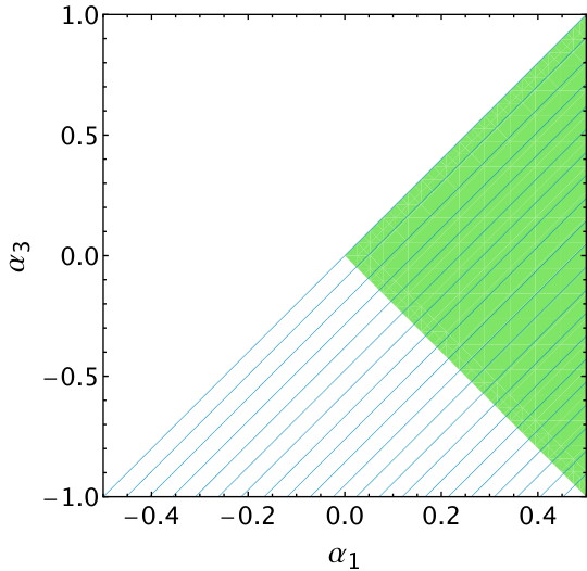
Moreover, our homogeneous bounds (19 – 21) are distinct from the order-of-magnitude causality bounds on $O(|\alpha_{3}|)$ Camanho:2014apa; Hamada:2018dde, which are derived assuming positivity of time delay and tree-level UV completion of the Einstein-Maxwell lagrangian. See also Goon:2016une; Camanho:2014apa for a nice discussion of detectability of superluminal propagation within an EFT, and how the Euler-Heisenberg lagrangian limit of the real-world QED avoids superluminality Drummond:1979pp.

It is interesting to compare the bounds (19 – 21) with the 4D calculation of the same processes retaining the Coulomb singularity in the $t\rightarrow 0$ limit

	$\displaystyle\mathcal{M}_{4D}^{\downarrow\downarrow}=$	$\displaystyle-\frac{s^{2}}{m_{\mathrm{Pl}}^{2}t}-\frac{s}{m_{\mathrm{Pl}}^{2}}+\frac{2s^{2}\left(2\alpha_{1}-\alpha_{3}\right)}{m_{\mathrm{Pl}}^{4}}\,,$		(22)
	$\displaystyle\mathcal{M}_{4D}^{\uparrow\uparrow}=$	$\displaystyle-\frac{s^{2}}{m_{\mathrm{Pl}}^{2}t}-\frac{s}{m_{\mathrm{Pl}}^{2}}+\frac{2s^{2}\left(2\alpha_{1}+\alpha_{3}\right)}{m_{\mathrm{Pl}}^{4}}\,,$		(23)
	$\displaystyle\mathcal{M}_{4D}^{\uparrow\downarrow}$	$\displaystyle=-\frac{s^{2}}{m_{\mathrm{Pl}}^{2}t}-\frac{s}{m_{\mathrm{Pl}}^{2}}+\frac{4s^{2}\alpha_{2}}{m_{\mathrm{Pl}}^{4}}\,,$		(24)

where the up and down arrows represent the two choices of real linear polarizations.⁶⁶ 6 We use real linear polarizations because they correspond to crossing symmetric amplitudes Bellazzini:2015cra; Bellazzini:2016xrt, up to the terms due to the Coulomb singularity. The lesson is that our 4D-regulated calculation, which works with 3D Lorentz invariance of the cylinder, teaches us which finite parts we are allowed to retain for the positivity bounds: throw away the $s^{2}/t$ singularity, the finite $O(s)$ term, but retain precisely the $O(s^{2})$ term.

This immediately prompts us to expect a continuous set of positivity bounds associated with arbitrary linear polarizations $|c_{1,2}\rangle=(c_{\theta_{1,2}}|\uparrow_{1,2}\rangle+s_{\theta_{1,2}}|\downarrow_{1,2}\rangle)$, namely

$$\alpha_{3}(c_{2\theta_{1}}+c_{2\theta_{2}})+4\alpha_{1}c^{2}_{\theta_{1}+\theta_{2}}+4\alpha_{2}s^{2}_{\theta_{1}+\theta_{2}}>0\,,$$

(25)

where $c_{\theta}=\cos\theta$ and $s_{\theta}=\sin\theta$. We will check the bounds (25) from arbitrary linear combinations with our controlled, IR-regulated method in future work.

The leading higher-dimensional corrections $\alpha_{i}$ in the 4D Einstein-Maxwell EFT (11) modify the black hole extremality condition to Kats:2006xp

$$\left(\frac{\sqrt{2}|Q|}{M/m_{\mathrm{Pl}}}\right)_{\mathrm{extr.}}=1+\frac{4}{5}\frac{(4\pi)^{2}m_{\mathrm{Pl}}^{2}}{M^{2}}(2\alpha_{1}-\alpha_{3})>1\,,$$

(26)

where $M$ is the black hole mass and $Q$ its charge (including the gauge coupling), and we work around $M\simeq Qm_{\mathrm{Pl}}\sqrt{2}$. Remarkably, on the right-hand side of this expression one finds the same combination $2\alpha_{1}-\alpha_{3}$ bounded to be positive by (19). Therefore, positivity bounds imply a greater charge-to-mass ratio for extremal black holes than in pure general relativity coupled minimally to an abelian $U(1)$ gauge theory. The lighter the extremal black hole, the larger the charge-to-mass ratio. Extremal black holes within the validity of the 4D EFT, i.e. whose Schwarzschild radius $r_{s}=M/4\pi m_{\mathrm{Pl}}^{2}$ is larger than $1/\Lambda_{UV}$, are therefore self-repulsive.

The positivity bound (19) implies the mild form of the WGC ArkaniHamed:2006dz, which states that a consistent theory of quantum gravity must contain massive charged states in the spectrum with $|q|>m/(\sqrt{2}m_{\mathrm{Pl}})$: the extremal black holes of (26) are such states. As a result, the paradox of stable extremal black holes has evaporated, since extremal black holes are no longer kinematically forbidden to decay into smaller black holes. Indeed, an extremal black hole of mass $M$ and charge $Q$ cannot decay into states that all have larger mass-to-charge ratio, since the spectrum of masses and charges $(m_{i},q_{i})$ is constrained by $M>\sum_{i}m_{i}$ and $Q=\sum_{i}q_{i}$, whereas $\sum_{i}m_{i}=\sum_{i}|q_{i}|m_{i}/|q_{i}|>M$ which would be a contradiction. This argument is evaded precisely by decay products that contain one smaller extremal black hole, which has smaller mass-to-charge ratio (26) because of the positivity bound (19).

Since the same combination of EFT coefficients, $2\alpha_{1}~-~\alpha_{3}$, enters the Wald entropy shift Cheung:2018cwt; Hamada:2018dde, our positivity bound (19) implies a larger black hole entropy as well.⁷⁷ 7 Positivity bounds of even higher-derivative terms Bellazzini:2015cra imply positive shift in the Kerr black hole entropy, too Reall:2019sah. Notice, however, that the reverse is not true. Requiring that the shift of the Wald entropy (of electrically charged black holes) is positive as a starting point Cheung:2018cwt does not produce the same bounds on $\alpha_{1}$ and $\alpha_{3}$, and says nothing about $\alpha_{2}$; while (19) is reproduced by demanding a positive entropy shift Cheung:2018cwt; Hamada:2018dde, the conditions (20) $2\alpha_{1}+\alpha_{3}>0$, (21) $\alpha_{2}>0$, and (25) are not.

Our IR-regulated positivity bounds can now be used to constrain scalar theories, e.g. the EFT of axions or modified gravity theories, that have a massless graviton in the spectrum.⁸⁸ 8 Positivity bounds applied to the Lorentz invariant EFT of massive gravity had a dramatic impact Bellazzini:2017fep. Let us consider for instance

$$\mathcal{L}=-\frac{1}{2}(\partial\phi)^{2}+\frac{a}{4f^{4}}(\partial\phi)^{4}+\ldots\,.$$

(27)

Without gravity, the positivity bounds would imply $a>0$ Adams:2006sv, and one could expect the same bound to hold as long as $f\ll m_{\mathrm{Pl}}$. However, what about the case $f\gg m_{\mathrm{Pl}}$? In fact, even for the case $f\ll m_{\mathrm{Pl}}$, things are not completely obvious in modified gravity theories.

For example, in the cosmological context a $P(X)$ theory is usually considered with a decay constant $f$ not too far from $\sqrt{m_{\mathrm{Pl}}H}\equiv\Lambda_{2}\ll m_{\mathrm{Pl}}$, where $H$ is the Hubble constant. However, the limit $t\rightarrow 0$ is an IR limit where the exchanged momentum goes to zero, so that intermediate massless particles such as the graviton affect macroscopic distances.⁹⁹ 9 Incidentally, this is why we believe the assumptions in Baumann:2015nta are not fully justified, since the graviton is probing curved spacetime regions even at large $s$. Even if one regulates the IR limit with the largest scale in the problem and takes $t\sim H^{2}$, the graviton Coulomb singularity (1) would give a contribution to the forward scattering which is at least as large as the one that we want to retain, i.e. $O(s^{2}/{m_{\mathrm{Pl}}^{2}H^{2}})=O(s^{2}/f^{4})$, thus spoiling the argument that leads to $a>0$. The same issue was originally pointed out in the context of 4D massive gravity Bellazzini:2017fep, where the intermediate transverse graviton competes with the galileon modes for the contribution to the $a^{\pi\pi}\sim m_{g}^{2}/\Lambda_{3}^{6}\sim 1/(m_{\mathrm{Pl}}^{2}H^{2})$ for a graviton mass $m_{g}\sim H$.

In the case of 4D massless gravity studied in this paper, after compactifying to $D=3$ there is no Coulomb singularity, while even if the series of gravitational KK modes (6) is formally logarithmically divergent, it can actually be removed in the subtracted dispersion relation (10). The left-hand side of (10) is thus finite and dominated by the contact terms, and since neither the dilaton nor the graviphoton contribute at leading order to the $s^{2}$-term in the forward $\phi\phi\rightarrow\phi\phi$ scattering, we conclude that in fact

$$a>0$$

(28)

holds true in any weakly coupled UV completion of an EFT of the type (27), such as $P(X)$ theories coupled to gravity, and in fact even for axions with $f\gg m_{\mathrm{Pl}}$ should their cutoff $\Lambda_{UV}=g_{*}f$ be smaller than the Planck mass.

More interesting conclusions apply to weakly broken galileons Nicolis:2008in; Pirtskhalava:2015nla. Let us consider for example

$$\mathcal{L}=-\frac{1}{2}(\partial\pi)^{2}-\frac{1}{2\Lambda_{3}^{3}}(\partial\pi)^{2}\square\pi+\frac{1}{4\Lambda_{2}^{4}}(\partial\pi)^{4}+\ldots\,,$$

(29)

where one can imagine the natural situation where $\Lambda_{2}\gg\Lambda_{3}$ since $(\partial\pi)^{4}$ weakly breaks the Galilean symmetry whereas $(\partial\pi)^{2}\square\pi$ is an invariant. It was shown indeed that the hierarchy

$$\Lambda_{2}^{4}\simeq H^{2}m_{\mathrm{Pl}}^{2}\,,\qquad\Lambda_{3}^{3}\simeq H^{2}m_{\mathrm{Pl}}\,,$$

(30)

is stable under the loop corrections due to gravity that break the galileon symmetry Pirtskhalava:2015nla, and in fact even larger values of $\Lambda_{2}$ such as $(Hm_{\mathrm{Pl}}^{2})^{1/3}$ are in principle consistent.

However, as estimated in Nicolis:2009qm; Bellazzini:2016xrt and calculated in detail in Bellazzini:2017fep, the scales $\Lambda_{2}$ and $\Lambda_{3}$ cannot be arbitrarily separated while keeping the cutoff $\Lambda_{UV}$ fixed in a theory without gravity, because the integrand under the dispersion relations (4) is strictly positive and it gives the following beyond positivity bound Bellazzini:2017fep:

$$a^{\pi\pi}=\frac{1}{\Lambda_{2}^{4}}>\frac{2}{\pi}\int^{\Lambda_{UV}^{2}}\frac{ds}{s^{3}}\mathrm{Im}\mathcal{M}^{\pi\pi}(s)\propto\frac{1}{16\pi^{2}}\frac{\Lambda_{UV}^{8}}{\Lambda_{3}^{12}}\,.$$

(31)

We can now see that a similar bound survives even when the graviton is dynamical if the UV completion is assumed to be weakly coupled (at least up to $\Lambda_{2}$). Following the arguments of the previous sections, we can subtract the gravitational KK modes after the 3D compactification, and then extract the following bound

$$\frac{1}{\Lambda_{2}^{4}L}>\frac{2}{\pi}\int^{\Lambda_{UV}^{2}}\frac{ds}{s^{3}}\mathrm{Im}\widetilde{\mathcal{M}}^{\pi\pi}(s)>\frac{c}{16\pi^{2}}\frac{\Lambda^{8}_{UV}}{L\Lambda_{3}^{12}}\,,$$

(32)

where in the last inequality we used the optical theorem and retained the contribution to the inelastic cross-section into two galileon KK modes $\pi_{k}$, $\sum_{k,m_{k}<\Lambda_{UV}}\sigma(\pi\pi\rightarrow\pi_{k}\pi_{k})$. The constant $c=O(10^{-4})$ is an inessential numerical factor resulting from integrating over the phase space and then along the branch cut. Loop corrections to the $s^{2}$-coefficient on the left-hand side of the dispersion relation are either very small or have been subtracted. The bound (32) nicely reproduces the scaling from the calculation without gravity in (31). As a consequence, the hierarchy (30) between $\Lambda_{2}$ and $\Lambda_{3}$, which is stable because of symmetries, in fact requires an extremely small cutoff

$$\Lambda_{UV}<\left(H^{3}m_{\mathrm{Pl}}\right)^{1/4}\left(\frac{16\pi^{2}}{c}\right)^{1/8}\sim\frac{1}{10^{7}\,\mathrm{km}}$$

(33)

in order to be consistent with the beyond positivity bound (32) that applies in a gravity theory. Vainshtein screening Vainshtein:1972sx is no longer a valid EFT argument at scales shorter than $\Lambda_{UV}^{-1}$ Nicolis:2004qq; Bellazzini:2016xrt because operators with arbitrarily more derivatives per field insertion become large, non-suprisingly, since new degrees of freedom are excited at $\Lambda_{UV}$.

It would be interesting to apply these new and powerful beyond positivity bounds to other general and still structurally robust EFTs of modified gravity Santoni:2018rrx.

In this section we argue how positivity bounds can be extended to the case of spacetimes which are barely $dS_{4}$ (or $AdS_{4}$), as appears to be the case in our universe with a 4D cosmological constant $\Lambda_{4}$ that is very close to the scale of the neutrino masses. One trivial way would be to assume that we can vary $\Lambda_{4}$ down to zero while the EFT coefficients we are interested in depending very little on such a change. We entertain instead another possibility, where $\Lambda_{4}$ is held fixed and less relevant or even marginal operators (e.g. Yukawa couplings) are varied.

It was shown in ArkaniHamed:2007gg that the Standard Model coupled to gravity has a landscape of 3D vacua which is accessible by varying the properties of neutrinos (or the value of $\Lambda_{4}$, or both) by just $O(1)$. One could for example vary the mass of the lightest neutrino, or the type (Dirac vs Majorana), or the mass splitting squared $\Delta m_{12}^{2}$, etc.. As these parameters are varied one gets $dS_{3}$ or $AdS_{3}$ solutions (times the compact dimension) which are energetically favored over $dS_{4}$. Importantly, a flat 3D Minkowski solution (times the compact dimension) can be energetically favorable as well. This can be reached for example by varying $\Delta m_{12}^{2}$ from $8\cdot 10^{-5}\text{ eV}^{2}$ to $1.5\cdot 10^{-5}\text{ eV}^{2}$ for Majorana neutrinos ArkaniHamed:2007gg. Tuning the theory with such a value, we can run again the positivity arguments derived in the previous sections to constrain the coefficients $a$ of, say, $a\,e^{4}(F_{\mu\nu})^{4}/\Lambda_{UV}^{4}$, which is obtained by integrating out massive charged states at the UV scale $\Lambda_{UV}$. Since the neutrinos are neutral and weakly coupled, one natural expectation is that changing e.g. $\Delta m^{2}_{12}$ while holding everything else fixed, will not dramatically backreact on the value of $a$, that is $a(\Delta m_{12}^{2})=a(\Delta m_{12}^{2}|_{SM})+O(\delta\Delta m_{12}^{2}/\Lambda_{UV})^{2}$. Alternatively, if the see-saw scale $\Lambda_{\nu}$ for generating Majorana neutrino masses, $m_{\nu}\sim v^{2}/\Lambda_{\nu}$, is much higher than the scale $\Lambda_{UV}$ we are interested in, then the contribution from particles at $\Lambda_{\nu}$ to the parameter $a$ is quickly overrun by the physics at $\Lambda_{UV}$. One would thus conclude that $a>0$ even in $dS_{4}$ with a finite $\Lambda_{4}$, within an accuracy $O(\delta\Delta m_{12}^{2}/\Lambda_{UV}^{2},\Lambda_{UV}^{4}/\Lambda_{\nu}^{4})$.

The same logic can be applied to bound modified gravity theories, for example $P(X)$ theories, assuming that changing e.g. $\Delta m_{12}^{2}$ (or the neutrino physics at $\Lambda_{\nu}$) does not change the cosmological constant $\Lambda_{4}$ by orders of magnitude. For example, one could imagine that $\Lambda_{4}$ is obtained by tuning various UV parameters against each other, possibly associated with scales even higher than $\Lambda_{\nu}$, so that they would impact the change in the coefficient of the IR irrelevant operators even less.

We worked with a specific example related to the Standard Model coupled to gravity, but the idea is general and can be easily adapted to other cases, adding for example particles that are not coupled to the Standard Model and yet contribute to the vacuum selection through their Casimir energies.

In this paper we derived new amplitudes’ positivities in quantum gravity in four dimensions. We showed how to regulate and subtract the gravitational Coulomb singularity in the forward elastic limit by putting the theory on a cylinder, using its 3D residual Lorentz invariance, and then restoring to 4D spacetime. This method allowed us to extract positivity bounds on the $s^{2}$-coefficient of the EFT amplitudes removing the $t$-channel graviton singularity in a controlled way. Remarkably, the resulting positivity bounds are generically different than those obtained in flat space without gravity. This is due to the contribution to the amplitudes from the dilaton and the graviphoton (on top of the contact terms from the non-dynamical metric), which remain dynamical even on the cylinder and leave their finite gravitational footprint in the 4D limit.

As an important application we studied the Einstein-Maxwell EFT and showed that the positivity bounds imply stronger inequalities than for the Euler-Heisenberg lagrangian. In turn, the bounds imply that extremal black holes have a charge-to-mass ratio larger than one, which is approached from above as the mass is increased. This provides an S-matrix proof of the mild form of the WGC since it implies that extremal black holes are self-repulsive, $|Q|>M$ in suitable units, and unstable to decay to smaller black holes. The amplitudes’ positivity imply as well that the Wald entropy shift due to the leading higher-dimensional operators is always positive.

In the context of the ‘‘swampland’’ program, these are perhaps somewhat negative results, since they lower the expectations that the WGC is useful to chart the landscape of consistent theories of quantum gravity. We employed only very general, basic S-matrix principles, and yet we have been able to show that extremal black holes are no longer kinematically stable thanks to the higher-dimensional operators generated by ‘‘any’’ weakly coupled UV completion with a consistent S-matrix. Of course, it may be that string theory is the only UV completion with such a canonical S-matrix.¹⁰¹⁰ 10 We note that the logical possibility exists that violation of our bounds points instead towards a fundamental obstruction to flat 3D compactifications, no matter how large the radius of the compact dimension is taken.

Given our bounds (19 – 21) on the Einstein-Maxwell EFT coefficients $\alpha_{i}$, one could try to follow the strategy of Cheung:2014ega; Chen:2019qvr; Andriolo:2018lvp, that is, to see whether the established bounds imply specific constraints on microscopic QFT models with $U(1)$ massive and charged particles that are integrated out to generate the $\alpha_{i}$. Such a general program faces, however, an obstruction because in 4D there are charge-independent and UV-sensitive contributions to the $\alpha_{i}$ from graviton loops (or dilaton, graviphoton, and KK-mode loops in the IR-regulated theory on the cylinder), which are not calculable in the QFT (i.e. they require knowledge of the details of the UV completion of quantum gravity). One could perhaps make some progress in this direction with the extra assumption that such purely gravitational UV contributions are somehow small Cheung:2014ega.

Another future direction is the exploration of the effective theory of $p$-forms coupled to gravity and whether the extremality conditions for black branes are related to the positivity bounds in quantum gravity once higher-dimensional operators are included in the EFT. The case of a zero form $\phi$, an axion, would be extremely important phenomenologically as the analog WGC could reveal an obstruction in taking transplanckian decay constants.

We considered other important applications in cosmology within the context of modified gravity, such as the positivity bound on the leading shift-symmetric operator for scalars coupled to gravity, like e.g. axions, $P(X)$ theories, and galileons. In particular, we found that perturbative UV completions of galileons can be consistent with the (beyond) positivity bounds in a theory with a massless graviton only if the cutoff of the theory is at least as small as $\mathrm{few}\times(H^{3}m_{\mathrm{Pl}})^{1/4}$. We have also discussed how positivity bounds can be extended to dS spacetime with a small cosmological constant by varying e.g. the properties of neutrinos.

References

- (1) A. Adams, N. Arkani-Hamed, S. Dubovsky, A. Nicolis, and R. Rattazzi, “Causality, analyticity and an IR obstruction to UV completion,” JHEP 10 (2006) 014, hep-th/0602178.
- (2) B. Bellazzini, “Softness and amplitudes positivity for spinning particles,” JHEP 02 (2017) 034, 1605.06111.
- (3) Z. Komargodski and A. Schwimmer, “On Renormalization Group Flows in Four Dimensions,” JHEP 12 (2011) 099, 1107.3987.
- (4) M. A. Luty, J. Polchinski, and R. Rattazzi, “The -theorem and the Asymptotics of 4D Quantum Field Theory,” JHEP 01 (2013) 152, 1204.5221.
- (5) N. Arkani-Hamed, L. Motl, A. Nicolis, and C. Vafa, “The String landscape, black holes and gravity as the weakest force,” JHEP 06 (2007) 060, hep-th/0601001.
- (6) C. Cheung and G. N. Remmen, “Infrared Consistency and the Weak Gravity Conjecture,” JHEP 12 (2014) 087, 1407.7865.
- (7) W.-M. Chen, Y.-t. Huang, T. Noumi, and C. Wen, “Unitarity bounds on charged/neutral state mass ratio,” 1901.11480.
- (8) M. Froissart, “Asymptotic behavior and subtractions in the Mandelstam representation,” Phys. Rev. 123 (1961) 1053–1057.
- (9) A. Martin, “Extension of the axiomatic analyticity domain of scattering amplitudes by unitarity. 1.,” Nuovo Cim. A42 (1965) 930–953.
- (10) M. Chaichian and J. Fischer, “Higher Dimensional Space-time and Unitarity Bound on the Scattering Amplitude,” Nucl. Phys. B303 (1988) 557–568.
- (11) M. Chaichian, J. Fischer, and Yu. S. Vernov, “Generalization of the Froissart-Martin bounds to scattering in a space-time of general dimension,” Nucl. Phys. B383 (1992) 151–172.
- (12) C. Cheung, J. Liu, and G. N. Remmen, “Proof of the Weak Gravity Conjecture from Black Hole Entropy,” JHEP 10 (2018) 004, 1801.08546.
- (13) Y. Hamada, T. Noumi, and G. Shiu, “Weak Gravity Conjecture from Unitarity and Causality,” 1810.03637.
- (14) X. O. Camanho, J. D. Edelstein, J. Maldacena, and A. Zhiboedov, “Causality Constraints on Corrections to the Graviton Three-Point Coupling,” JHEP 02 (2016) 020, 1407.5597.
- (15) G. Goon and K. Hinterbichler, “Superluminality, black holes and EFT,” JHEP 02 (2017) 134, 1609.00723.
- (16) I. T. Drummond and S. J. Hathrell, “QED Vacuum Polarization in a Background Gravitational Field and Its Effect on the Velocity of Photons,” Phys. Rev. D22 (1980) 343.
- (17) B. Bellazzini, C. Cheung, and G. N. Remmen, “Quantum Gravity Constraints from Unitarity and Analyticity,” Phys. Rev. D93 (2016), no. 6 064076, 1509.00851.
- (18) Y. Kats, L. Motl, and M. Padi, “Higher-order corrections to mass-charge relation of extremal black holes,” JHEP 12 (2007) 068, hep-th/0606100.
- (19) H. S. Reall and J. E. Santos, “Higher derivative corrections to Kerr black hole thermodynamics,” 1901.11535.
- (20) B. Bellazzini, F. Riva, J. Serra, and F. Sgarlata, “Beyond Positivity Bounds and the Fate of Massive Gravity,” Phys. Rev. Lett. 120 (2018), no. 16 161101, 1710.02539.
- (21) D. Baumann, D. Green, H. Lee, and R. A. Porto, “Signs of Analyticity in Single-Field Inflation,” Phys. Rev. D93 (2016), no. 2 023523, 1502.07304.
- (22) A. Nicolis, R. Rattazzi, and E. Trincherini, “The Galileon as a local modification of gravity,” Phys. Rev. D79 (2009) 064036, 0811.2197.
- (23) D. Pirtskhalava, L. Santoni, E. Trincherini, and F. Vernizzi, “Weakly Broken Galileon Symmetry,” JCAP 1509 (2015), no. 09 007, 1505.00007.
- (24) A. Nicolis, R. Rattazzi, and E. Trincherini, “Energy’s and amplitudes’ positivity,” JHEP 05 (2010) 095, 0912.4258. [Erratum: JHEP11,128(2011)].
- (25) A. I. Vainshtein, “To the problem of nonvanishing gravitation mass,” Phys. Lett. 39B (1972) 393–394.
- (26) A. Nicolis and R. Rattazzi, “Classical and quantum consistency of the DGP model,” JHEP 06 (2004) 059, hep-th/0404159.
- (27) L. Santoni, E. Trincherini, and L. G. Trombetta, “Behind Horndeski: structurally robust higher derivative EFTs,” JHEP 08 (2018) 118, 1806.10073.
- (28) N. Arkani-Hamed, S. Dubovsky, A. Nicolis, and G. Villadoro, “Quantum Horizons of the Standard Model Landscape,” JHEP 06 (2007) 078, hep-th/0703067.
- (29) S. Andriolo, D. Junghans, T. Noumi, and G. Shiu, “A Tower Weak Gravity Conjecture from Infrared Consistency,” Fortsch. Phys. 66 (2018), no. 5 1800020, 1802.04287.
- (30) M. Ciafaloni, “Selfconsistent scattering matrix in (2+1) gravity,” Phys. Lett. B291 (1992) 241–245.
- (31) G. ’t Hooft, “Nonperturbative Two Particle Scattering Amplitudes in (2+1)-Dimensional Quantum Gravity,” Commun. Math. Phys. 117 (1988) 685.
- (32) S. Deser, J. G. McCarthy, and A. R. Steif, “UltraPlanck scattering in D = 3 gravity theories,” Nucl. Phys. B412 (1994) 305–319, hep-th/9307092.
- (33) M. Zeni, “Forward scattering in (2+1) quantum gravity,” Class. Quant. Grav. 10 (1993) 905–911.
- (34) D. N. Kabat and M. Ortiz, “Eikonal quantum gravity and Planckian scattering,” Nucl. Phys. B388 (1992) 570–592, hep-th/9203082.
- (35) G. ’t Hooft, “Graviton Dominance in Ultrahigh-Energy Scattering,” Phys. Lett. B198 (1987) 61–63.
- (36) S. Deser and P. van Nieuwenhuizen, “One Loop Divergences of Quantized Einstein-Maxwell Fields,” Phys. Rev. D10 (1974) 401.