Bayesian and frequentist approaches to resonance searches
Abstract
We investigate Bayesian and frequentist approaches to resonance searches using a toy model based on an ATLAS search for the Higgs boson in the diphoton channel. We draw pseudo-data from the background only model and background plus signal model at multiple luminosities, from to . We chart the change in the Bayesian posterior of the background only model and the global p-value. We find that, as anticipated, the posterior converges to certainty about the model as luminosity increases. The p-value, on the other hand, randomly walks between and if the background only model is true, and otherwise converges to . After briefly commenting on the frequentist properties of the posterior, we make a direct comparison of the significances obtained in Bayesian and frequentist frameworks. We find that the well-known look-elsewhere effect reduces local significances by about . We furthermore find that significances from our Bayesian framework are typically about smaller than the global significances, though the reduction depends on the prior, global significance and integrated luminosity. This suggests that even global significances could significantly overstate the evidence against the background only model. We checked that this effect — the Bayes effect — was robust with respect to fourteen choices of prior and investigated the Jeffreys-Lindley paradox for three of them.
I Introduction
Resonances are narrow peaks in the invariant mass distributions of pairs of particles detected in, for example, a collider experiment. As a resonance originates from the on-shell production and subsequent decay of a massive particle, a new resonance indicates the discovery of a new particle, as was the case in 2012 when the Higgs boson was discoveredAad et al. 2012; Chatrchyan et al. 2012 at the Large Hadron Collider (LHC). New resonances typically lie above a background of events originating from well-understood physical processes. Unfortunately, upwards statistical fluctuations in that background can, by chance, imitate a resonance. Thus to discover a particle we must distinguish fluctuations from genuine resonances.
The ATLAS and CMS experiments at the LHC use null hypothesis significance testing to determine whether there is a new resonance in an invariant mass distribution. This methodology, reviewed in sec. III, invokes hypothetical pseudo-experiments conducted with no resonance. If the fraction of pseudo-experiments that would result in data at least as extreme as that observed (the so-called p-value) lies below a threshold, we reject the possibility that there is no resonance, and possibly herald a discovery. In light of historical (see e.g., ref. Rozeboom 1960) and recent (see e.g., ref. Benjamin et al. 2017) criticism, we recently advocatedFowlie 2017; Fowlie 2018 an alternative methodology based on Bayes factors, reviewed in sec. IV. In this methodology, we consider only the observed data, and directly compare the plausibility of that data in a model with a resonance to that in one without one. This allows us to calculate, amongst other things, the posterior probability of the background only model.11 1 As discussed further in sec. IV, we assume throughout that the background and signal models are a priori equally plausible.
In ref. Fowlie 2017 we considered the infamous anomaly, when ATLAS and CMS saw hints of a resonance in the invariant mass distribution of photons at . This would have been a historic discovery and it generated considerable activity (see e.g., ref. Strumia 2016 for a review). Looking at ATLAS dataATLAS 2015; Aaboud et al. 2016, we found that whilst the p-value of about appeared suggestive, for our choices of priors the posterior of the background model was in fact about . The anomaly ultimately disappeared once more data was collectedATLAS 2016. Similarly, in ref. Fowlie 2018, we considered a hint for a resonance in the energy spectrum of electrons measured by the DAMPE satelliteAmbrosi et al. 2017. The hint could be the first direct evidence for dark matter. We again found that for our choices of priors the posterior of the background, about , was significantly greater than the p-value, about .
With these two cases in mind, in this work we compare the behavior of the posterior of the background and the p-value in resonance searches. In sec. II we present a toy example of a resonance search based on one in which ATLAS discovered the Higgs bosonAad et al. 2013. We review the frequentist and Bayesian methods for analyzing this toy problem in sec. III and sec. IV, respectively, and apply them to real and pseudo-data from it in sec. V, showing how results change as the dataset grows (see ref. Schönbrodt et al. 2017 for a similar analysis in a different context), and differences between the statistical approaches. Resonance searches are tests of point null hypotheses. Historically, such tests drew considerable attention and remain controversial (see e.g., ref. Lindley 1957; Shafer 1982; Bernardo 1980; Sprenger 2013; Berger and Delampady 1987; Trotta 2007; Robert 2014; Cousins 2017) due to the Jeffreys-Lindley paradoxJeffreys 1939; Lindley 1957.
We find in sec. V.4 that the posterior of the background only model is typically orders of magnitude greater than the p-value.22 2 Ref. Johnson 2013 reaches a similar conclusion in an extremely crude analysis of the Higgs discovery. This echoes criticisms that p-values overstate the evidence for effects in other fields (see e.g., ref. Edwards et al. 1963; Berger and Sellke 1987; Benjamin et al. 2017). Despite arguments in e.g., ref. Lyons 2014; Senn 2001 that such comparisons are akin to comparing heights and weights, we feel that a comparison is justified as both the p-value (when interpreted in the manner of Fisher; see sec. III) and posterior aim to answer the same question: how strong is the evidence against the null hypothesis? The fact that p-values markedly differ from results of Bayesian methods does not, however, imply that p-values are wrong.
We do not in this work address in detail further criticisms of either methodology, e.g., the dependence of Bayes factors on choices of prior (see e.g., ref. Kass and Raftery 1995; Cousins 2008), though discuss prior sensitivity of our findings in sec. VI and the Jeffreys-Lindley paradox in sec. VII. We summarize our findings in sec. VIII.
II Toy problem — ATLAS diphoton search for a Higgs boson
We consider a historic ATLASAad et al. 2013 search for a Higgs boson in the diphoton channel at and with of integrated luminosity; this search contributed to the discovery of the Higgs boson in 2012. The inclusive observed spectrum is shown in fig. 1. The spectrum (red points) exhibits a suggestive resonance-like feature at . We consider two models for the data.
First, a background only model, , representing the background from known Standard Model (SM) processes other than a Higgs boson. ATLAS model the background by a Bernstein polynomial. This introduces several unknown coefficients and an unknown normalization that governs the overall expected background yield. So that we can perform millions of fits, we fix the coefficients and normalization to their best-fit values and thus omit all systematic uncertainties in the background, including parametric uncertainties in the Bernstein coefficients and uncertainties associated with that particular choice of functional form.
Second, a background plus signal model, . This is the background spectrum plus a narrow resonance, i.e., one with a width, , that is substantially narrower than the experimental resolution of about . We thus approximate the width as zero, . We know the expected amplitude of a resonance from an SM-like Higgs boson. We choose to model a Higgs-like signal with only two a priori unknown parameters: the mass of the Higgs, , and the amplitude of the signal relative to the SM, .
The observed data is a set of counts, with , in each of bins in diphoton invariant mass spanning . We denote the expected number of background events per bin by . In the signal model, the expected number of events is the sum of the expected number of background events and signal events, ,
| (1) |
The expected signal is scaled by the signal strength, , and itself depends on the Higgs mass by
| (2) |
where is the bin center, is the bin width, is the integrated luminosity, is the total production cross section, is the selection efficiency, and is the shape of the signal. We model the shape by a Gaussian centered at the Higgs mass, , with a width of , governed by the experimental resolution. We pick a Gaussian for simplicity; ATLAS in fact use a modified Crystal Ball function. We found heuristically by reproducing the ATLAS result at . The total background cross section, on the other hand, was about .
Thus the likelihood of the observed events is the product of Poisson likelihoods, one for each bin,
| (3) |
where and , are the expected and observed numbers of events in bin , respectively. We stress that this is a toy treatment of the problem, intended to capture only the major details, that omits e.g., systematic uncertainties or a detailed treatment of the selection efficiency and cross section as functions of the Higgs mass.
III Frequentist
In the frequentist framework, we construct a log likelihood ratio test-statistic,
| (4) |
where represents our experimental data and the hats indicate the best-fitting value of a parameter. The best-fitting signal strength cannot be negative, . Using the likelihood in eq. 3, we have that
| (5) | ||||
| (6) |
The frequentist quantities of interest are functions only of , which itself implicitly depends on and . To ensure that no signals are missed, we find the best-fit mass and signal strength inside every bin with an excess by Brent’s methodJones et al. 1; Brent 1973, using for that bin as a starting guess for the signal strength. Lastly, we select the best-fit mass and signal strength found from all the bins.
We use the test-statistic to calculate p-values with respect to a null hypothesis, which in this work is always the background only model. The global p-value is the probability of obtaining a test-statistic at least as extreme as that observed for any value of the Higgs mass, assuming that the background only model is true,
| (7) |
A local p-value, on the other hand, presupposes that we were testing only a specific value of the Higgs mass. The p-value is distributed as uniformly as possible under the background only modelBlocker and et al 2006. Thus, if we reject the background model only when the p-value lies below a threshold specified in advance,
| (8) |
the threshold is the type-1 error rate, i.e., the probability of rejecting the background model when it is true. The p-value itself though has no frequentist or Bayesian meaning: it is not an error rate or the probability of the background only modelGibbons and Pratt 1975. In high-energy physics, p-values are informally interpreted in the manner of FisherFisher 1925 as a continuous measure of evidence against the background only model, though discoveries traditionally require a p-value below about , corresponding to Lyons 2013.33 3 See ref. Hubbard and Bayarri 2003 for a discussion of this hybrid interpretation.
To calculate p-values, we make use of two formulas that are appropriate because our test-statistic is a log likelihood ratio between nested hypotheses (the signal plus background model contains the background model at ). For local p-values, we use an asymptotic formulaCowan et al. 2011 based on Wilks’ theoremWilks 1938; Chernoff 1954
| (9) |
where is the cumulative distribution function of a standard normal distribution. This presupposes that we were testing only the best-fitting Higgs mass, . For global p-values, we try a bootstrap technique: as discussed in sec. V we ultimately perform k pseudo-experiments at several luminosities, repeating the minimization in eq. 4 each time. We count the fraction of pseudo-experiments that result in a test-statistic greater than or equal to that observed.44 4 In other words, we recycle our pseudo-experiments. First, we use them to simulate the distribution of the test-statistic under the null hypothesis. Second, we use them in our comparisons of Bayesian and frequentist techniques. If the resulting global p-value lies below , we make use of the Gross-Vitells techniqueGross and Vitells 2010, which should be more precise than bootstrap in that regime,
| (10) |
where is a random variate from a chi-squared with one degree of freedom and is an a priori unknown parameter.55 5 Under the asymptotic conditions required by the Gross-Vitells method, doesn’t depend on the luminosity. We determined by counting the number of upcrossings of the test-statistic between and in k Monte-Carlo (MC) simulations. Thus this formula accounts for a one-dimensional look-elsewhere effect for the Higgs mass in the range to .66 6 Note that ATLASAad et al. 2012 corrected for look-elsewhere effects in the ranges and , whilst CMSChatrchyan et al. 2012 corrected for them in the ranges and . The narrower ranges reflected indirect constraints and exclusion limits from previous experiments and mitigated edge effects at the boundaries of the data. We checked that edge effects were absent by checking that the distribution of the log-likelihood ratio matched the expected asymptotic resultCowan et al. 2011 at the boundaries. We furthermore checked that narrowing the interval to did not qualitatively affect our results. This was unaccounted for by eq. 9 because the likelihood’s dependence on the Higgs mass vanishes on the boundary, breaking an assumption of Wilks’ theorem.
Finally, we convert p-values to Z-values, as is conventional, using a one-tailed Gaussian rule,
| (11) |
IV Bayesian model comparison
We consider the probability of the data in each model — the so-called Bayesian evidence. For the signal model, we must marginalize the a priori unknown Higgs mass and signal strength,
| (12) |
where the second factor in the integrand is our choice of prior density for the Higgs mass and signal strength. We perform the integration by adaptive quadraturePiessens et al. 1983; Jones et al. 1, treating the bin centers of the five bins with the most significant excesses as special points. For the background model, it is trivial, as there are no free parameters, so the evidence is given directly by eq. 6.
Clearly, the evidence for the signal model depends upon our choice of prior. For the mass, we focused on the narrow range searched by ATLAS of to — although choices that extend this range could reflect prior belief, they would simply dilute the evidence for the signal model. Since it did not span multiple decades, we picked a flat prior. For the signal strength, we imagined a scenario in which we expected it to be somewhat close to the SM prediction of , though could deviate by a couple of orders of magnitude. We supposed that we were ignorant of the magnitude of this deviation and thus picked a prior that was flat in logarithmic space between and . This prior does not favor any particular order of magnitude, ; however, the prior predictive for the best-fit signal strength could favor particular magnitudes depending on the likelihood. We investigate several other choices of prior in sec. VI.
With the evidences, we calculate the Bayes factor (see e.g., ref. Kass and Raftery 1995 for a review),
| (13) |
This is the impact of the data on the relative plausibility of models and . As the luminosity grows, we expect the Bayes factor to increasingly favor the true modelChatterjee et al. 2018; Chib and Kuffner 2016. To facilitate a comparison with p-values, we find the posterior of the background model,
| (14) |
We can coherently incorporate relevant background information in our choices of priors for the models, and . From hereon we assume that the models are a priori equally plausible, , though if we had a reason for considering new physics relatively implausible, we could choose . In this work we compute posteriors to enable a comparison with p-values; however, we usually advocate reporting only Bayes factors, since they are independent of the priors for the models themselves.
We, furthermore, convert the posterior into a Z-value — which we call the Bayesian significance — using the rule in eq. 11. We do not advocate this in general and do so only to communicate our results to particle physicists so used to thinking of anomalies in terms of the number of sigmas.
There exists a bound on the rate at which we would be misled by the posterior about the true modelKerridge 1963. With two models under consideration that are equally plausible a priori, if model is correct, the chance that we find a posterior for that is less than a threshold is bounded by
| (15) |
The general bound depends on the number of models considered and the prior odds between the models.
For our toy problem, there exists a lower bound on the posterior of the background obtainable with any priors for the mass and signal strength (see ref. Delampady and Berger 1990 and references therein for further discussion of lower bounds on the posterior). The posterior is minimized when the priors select the best-fitting mass and strength, such that
| (16) |
where is the test-statistic defined in eq. 4.
There are two major causes of discrepancies between posteriors and p-values. First, the fact that the p-value considers the probability that the test-statistic exceeds a threshold, i.e, the probability of
| (17) |
rather than the probability of obtaining the observed data or observed test-statistic. To aid our comparisons between Bayesian and frequentist procedures, we thus compute the posterior of the background assuming this coarse-grained information, i.e., we calculate
| (18) |
In the Bayesian context, conditioning upon is strange as we should condition upon all that we know, i.e., the observed data itself. There is a gulf between knowing the data and knowing only that the data was in the set (see ref. Berger and Delampady 1987 for further discussion). This is useful though as if the models are equally plausible a priori,
| (19) |
where may be calculated using asymptotic formulae developed for frequentist applications. When the p-value is small, eq. 19 can be written as,
| (20) |
In this form it resembles Junk 1999; Read 2002 and Birnbaum’s measure of evidence in a binary experimentBirnbaum 1961; Birnbaum 1962. Under the signal model, is distributed as uniformly as possible, such that its median is about one half. Thus for small p-values the median coarse-grained posterior approximately equals twice the p-value.
The second major cause of discrepancies between posteriors and p-values is the so-called Occam effectMackay 2003. The evidence in eq. 12 may be thought of as the likelihood averaged upon the prior. If the prior typically poorly predicts the observed data by e.g., predicting signal strengths much greater than favored by data, the evidence would be automatically penalized by averaging, even if the prior permits a signal strength that successfully predicts the observed data. This means that the posterior for the signal model would typically be reduced by broadening the prior range for e.g., the signal strengthBartlett 1957.
IV.1 The Jeffreys-Lindley paradox
The Jeffreys-Lindley paradoxJeffreys 1939; Lindley 1957 demonstrates that a posterior and a p-value could result in opposite conclusions even in the asymptotic limit. The paradox results from the fact that the posterior corresponding to a particular p-value may depend on the sample size (i.e., integrated luminosity in the context of collider physics) such that the disagreement between the posterior and p-value could diverge as the sample size increases. The paradox prompted questions about the foundations of hypothesis testing; for commentary and attempted resolutions, see e.g., ref. Lindley 1957; Shafer 1982; Bernardo 1980; Sprenger 2013; Berger and Delampady 1987; Trotta 2007; Robert 2014; Cousins 2017.
In the example of the paradox in ref. Cousins 2017 we imagine Gaussian measurements of an unknown parameter, , with a sample mean . We consider two hypotheses: the null in which and an alternative in which . The sample mean is a sufficient statistic such that evidence for the null is simply a Gaussian evaluated at ,
| (21) |
where is the chi-squared. For the evidence for the alternative model, we must average the likelihood upon a prior for the unknown parameter, ,
| (22) |
The Bayes factor is given by their ratio,
| (23) |
As grows the exponential term in the integrand becomes sharply peaked at , such that we may make a Laplace approximation resulting in
| (24) |
The p-value, on the other hand, depends only on the chi-squared by for a one-sided test.
To create the paradox, we consider fixed chi-squared but increasing sample size. If is independent of , from eq. 24 we see that for fixed chi-squared the Bayes factor tends to zero as the sample size increases. Thus, despite an arbitrarily small p-value, the Bayes factor could overwhelmingly favor the null. To maintain a fixed chi-squared, however, the sample mean must scale as . This reflects the fact as we accumulate data we are sensitive to smaller effects.
V Results
V.1 Trajectories as we collect luminosity
We begin in fig. 2 by investigating the change in the p-value and posterior of the background as the integrated luminosity grows. First, we sampled data from the background only model, performing k pseudo-experiments at 50 luminosities between and . As we increased the luminosity, we added events to existing datasets, such that they were correlated. At each luminosity, we found the median and an equal-tailed interval for the posterior of the background model and the p-value. We found that the posterior increases monotonically from to as the luminosity increases, with a narrow interval (top left panel), i.e., as the luminosity grows, the true model is increasingly favored. The rate of convergence, however, is slow; it takes about before any strong preference for the background emerges. The p-value, on the other hand, makes a random walk, with a median of regardless of the luminosity (bottom left panel).
Second, we sampled data from the signal model assuming a signal strength and a mass , performing k pseudo-experiments at the same 50 luminosities. Surprisingly, the posterior first increases from , before rapidly decreasing to once the luminosity exceeds about (top right panel). The initial increase in the posterior is, however, mild; the median reaches about , which shouldn’t be considered worth more than a bare mentionJeffreys 1939. It occurs because below about Poisson fluctuations in the background of order provide an economical explanation of a signal-like feature as . The signal model isn’t strongly rewarded as it cannot provide a much better fit to the data; however, it is punished by the Occam effect as it wastes prior probability at , which would typically result in signals that were not observed. This results in a mild preference for the background model. Above about , fluctuations in the background cannot explain a signal as , and thus the posterior of the background decreases to , as expected. In other words, at large luminosities, the reward from a better fit overcomes the Occam effect.
The p-value, on the other hand, decreases monotonically to (lower right panel) though within a substantial interval. As the signal and background models are similar at small luminosities, the interval for the p-value at small luminosities is similar to that when the background model is true. We show a random subset of MC realizations (dashed lines), illustrating possible trajectories of the p-value and posterior.
V.2 Sampling properties of p-values and posteriors
We continue by performing k pseudo-experiments under the background only model and signal model assuming a signal strength and a mass , at integrated luminosities of , , , , and , though this time the datasets are completely independent. In fig. 3 we show the resulting distributions of the posterior and p-value at . The posterior peaks at about under the signal and background models, though under the latter mildly greater posteriors are favored. Thus, even when the signal model is true, the posterior typically mildly favors the background model. The explanation is identical to that in sec. V.1: below about , a fluctuation in the background can mimic the signal whereas the signal model wastes prior probability at . The p-value on the other hand is flat under the background distribution, but peaks near under the signal model, with a substantial tail extending to . At , shown in fig. 4, the posterior under the background model peaks at about , with greater preference rare, and under the signal model, it peaks near , with a moderate tail. The p-value of course remains flat under the background distribution, but now sharply peaks near under the signal model.
V.3 Type-1 errors and power
In fig. 5 we consider the type-1 error associated with the posterior, i.e., if we placed a threshold on the posterior, what is the type-1 error rate? We see that this depends on the luminosity, though for all luminosities below posteriors of about , the type-1 error rate is substantially less than the posterior and the bound in eq. 15. Thus, although in the Bayesian framework we relinquish direct control over the type-1 error rate, we find no evidence that a threshold on the posterior would lead to significant type-1 error rates in this setting.77 7 We do not, however, necessarily recommend making a dichotomous decision, based on a threshold on the posterior or anything else.
In a similar manner, we investigated power — the probability of rejecting the background model when we generated data from the signal model with and . We show in fig. 6 that the ROC curves — the power versus the type-1 error rate — were extremely similar for the log likelihood ratio in eq. 4 and the posterior in eq. 14. They would thus result in similar type-2 error rates for a fixed type-1 rate when used as test-statistics in a hypothesis test. This is not surprising — it is consistent with the fact that we observed an approximately monotonic relationship between the posterior and log likelihood ratio in this setting and the fact that error rates are invariant under strictly monotonic transformations of the test-statistic.
V.4 The Bayes effect
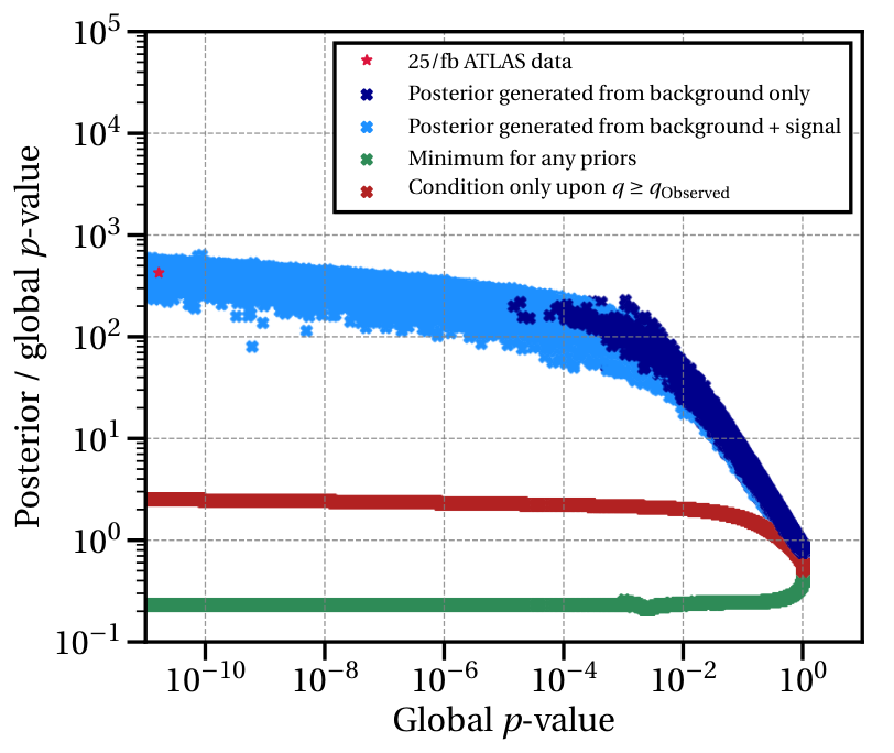
In fig. 7, we contrast the results from Bayesian and frequentist approaches. The ratios between the posterior of the background only model and p-value are scattered against the p-values from k pseudo-experiments at , , , , and (blue points). We do not find any significant differences in the relationship between p-value and posterior at different luminosities and thus scatter them together.88 8 One might, however, have anticipated a Jeffreys-Lindley-style paradoxLindley 1957; Jeffreys 1939. The effect does not occur with a logarithmic prior; see sec. VII for further discussion. The global p-values are significantly smaller than the associated posterior of the background by about for p-values smaller than about . Whilst both are extremely small, the global p-value from the data observed by ATLAS is about times smaller than the posterior (red star). We furthermore show that the minimum posterior obtainable with any priors for the Higgs mass and signal strength lies slightly below the global p-value (green points). We return to the issue of priors in sec. VI.
Lastly, we show the effect of conditioning only upon the fact that the test-statistic was greater than the observed test-statistic, eq. 17. This puts the exact experimental information used in the calculation of the p-value into the Bayesian one. We see that in this case the posteriors and p-values (red points) are similar, suggesting that this — and not the Occam effect, prior information or differences in interpretation of probability — may be the fundamental origin of the differences between the posteriors and p-values.
We convert posteriors and p-values to Z-values by the one-tailed rule in eq. 11. In fig. 8 (top panel) we show the difference between the global significance (i.e., the global p-value converted to a Z-value) and the Bayesian significance (i.e., the posterior of the background model converted to a Z-value) as a function of the global significance. We call this difference the Bayes effect, i.e.,
| (25) |
This can be interpreted as a calibration of global significances. For global significances greater than about the Bayes effect is at least and peaks at over when the global significance is about . Thus the Bayes effect means that in the Bayesian framework global significances of about vanish and even global significances of , the discovery threshold, reduce to about . The Bayes effect appears as important as the look-elsewhere effect in resonance searches (bottom panel) which reduces local significances by a similar amount.99 9 Our numerical results are consistent with the fact that the ratio of the global to local p-values — the trials factor — increases linearly with the local significance. The apparent contradiction with the fact that the change in significance decreases as the local significance increases stems from the non-trivial conversion to Z-values. We anticipated that the Bayes effect would be non-zero as we knew that the posterior and p-value would not be identical; however, we find the magnitude of the Bayes effect interesting, as it could change our interpretation of anomalies in resonance searches. There is spread in the Bayesian significance as it is a function of the entire dataset and not only the test-statistic. The Bayes effect occurs regardless of whether data were generated from the background (dark colors) or signal model (light colors) and at all luminosities under consideration.
As discussed in sec. III, global p-values greater than were calculated with a bootstrap technique and those smaller than that were calculated with Gross-Vitells. A minor discrepancy between the techniques is visible at the boundary at in fig. 7 (green points) and at in fig. 8 (bottom panel). The discrepancy — about in Z-value — originates from Monte-Carlo errors in the bootstrap technique and asymptotic approximations in Gross-Vitells.
Finally, it is tempting but risky to assume that the magnitude of the Bayes effect in this setting translates directly to other tests of the SM. Although a general result — the Vovk-Selke bound on the Bayes factorVovk 1993; Sellke et al. 2001 — indicates that effects at least as great as could be common, its assumptions may be violated in tests of the SM, as they are in this one. Thus whilst we expect a similar effect in any test of the SM and there might be some useful rules of thumb, the actual result must be problem specific and requires a full calculation. In this regard, the Bayes effect is similar to the look-elsewhere effect.

VI Sensitivity to our choices of prior


The posterior of the background only model depends upon choices of prior for the Higgs mass and signal strength. To check whether the Bayes effect was an artifact of our particular choices, we repeated our calculations at with thirteen alternative choices of prior:
- 0.
Our default choice; the priors described in sec. IV.
- 1.
We halved the breadth of the prior for the logarithm of the signal strength so that spanned to .
- 2.
We doubled the breadth of the prior for the logarithm of the signal strength so that spanned to .
- 3.
We picked a logarithmic prior for the Higgs mass.
- 4. – 5.
We picked a Gaussian prior for the order of magnitude of the signal strength, centered at . We made two choices for the width, and .
- 6.
We picked a flat prior for the signal strength, .
- 7. – 9.
We picked a fat-tailed distribution, a Cauchy truncated to allow only positive values, for the signal strength. We centered it at , representing prior knowledge that and made two choices for the width, and . We furthermore picked one representing prior information that was faulty: with a width .
- 10. – 12.
We picked a Gaussian prior for the Higgs mass, centered at . We made two choices for the width, and . We again picked one representing information that was faulty: with a width .
- 13.
Finally, we considered a prior representing accurate, precise prior information about the mass and strength: Gaussians centered at and with widths and , respectively.
The priors represented different possible states of knowledge about the Higgs mass and coupling strength; from vague knowledge, represented by broad priors, to specific information about their likely values, represented by distributions peaked at e.g., or . If we specified the prior for only the Higgs mass or signal strength, we used the choice of prior introduced in sec. IV for the other.
We show the resulting Bayes effects in fig. 9. We first consider vague priors (green colors). The Bayes effect shows mild dependence on the prior. For substantial global significances the effect is stronger for broader priors, e.g., the effect was biggest for a logarithmic prior on the signal strength between and (prior 2) and weakest for a log-normal prior that favored a particular order of magnitude (prior 4. – 5.) and the flat prior (prior 6). This was anticipated as the evidence for the signal model could be diluted by picking a broader prior, enhancing the posterior of the background model. Global significances of about , however, were always reduced by at least about . As it was so similar to the result from prior 0, we do not show the result for prior 3.
Second, we considered priors representing hypothetical specific prior knowledge about the Higgs mass or signal strength (red colors). In this case, the behavior depends strongly on whether data was generated under the signal or background model, since the latter may generate resonance-like features that do not agree with our prior knowledge for the mass and strength of the resonance. We find that for data generated under the signal model, specific correct knowledge reduces the Bayes effect, since it reduces the required tuning. For data generated under the background model, however, the Bayes effect could be amplified, as the posterior of the background is enhanced if the anomaly is not in accord with prior knowledge, regardless of its global significance. This resulted in substantial variation in the posterior associated with a particular global significance (see e.g., prior 7. – 9. and prior 10. – 12.).
If we had roughly known both the Higgs mass and signal strength in advance (prior 13), there would be only a minor Bayes effect under the signal model if the global significance was greater than about . The Bayes effect could, however, reduce global significances of about to nothing. Under the background model, the Bayes effect was potentially dramatic, reducing global significances of less than about to evidence against the signal model, though showed substantial variance.
Finally, we consider specific but faulty prior information. Under the signal model this enhances the posterior of the background and thus the Bayes effect, since the prior information conflicts with the observed resonance-like feature. For the prior centered at (prior 10. – 12.), the Bayes effect becomes dramatic, reducing global significances of to about .
We summarize the prior sensitivity of the Bayes effect in fig. 10. For the vague priors (top panel), the minimum and maximum effects are typically separated by less than about . For moderate global significances, the Bayes effect always reduces the significance by at least about . For the specific priors (bottom panel), the maximum effect is typically substantial, as specific information that conflicts with data drastically reduces the significance. We stress, however, that the minimum effect is typically greater than about ; negative Bayes effects that dramatically increase the significance are impossible. This is consistent with the fact that the minimum posterior achievable for any prior was only about a factor four smaller than the global p-value (fig. 7).
VII Sensitivity to the integrated luminosity and the Jeffreys-Lindley paradox

To investigate the paradox discussed in sec. IV.1, we repeated our calculations at , , , , and for three of our choices of prior for the signal strength: our default choice (prior 0), a logarithmic prior that favors no particular scale; a log-normal prior (prior 4. – 5.), which favors ; and a flat prior between and (prior 6). In fig. 11 we show the Bayes effect as we increase integrated luminosity for these three choices. We only consider data generated under the background only; we cannot easily consider fixed significance under the signal model as the significance increases as we increase luminosity. The logarithmic prior results in mild dependence on the luminosity. The Bayes effect, however, shows strong dependence on the luminosity for a log-normal and flat prior.
We can understand the absence of a paradox for a logarithmic prior by reconsidering the canonical example. In eq. 24, the Bayes factor’s explicit dependence on cancels for a logarithmic prior, , since it would result in . The fact that the Bayes factor no longer explicitly depends on is not surprising as the logarithmic prior is invariant under changes of scale, and by considering more data at fixed chi-squared we are probing smaller scales. This result in fact holds exactly in eq. 23 as for a logarithmic prior that equation is independent of at fixed chi-squared, which may be shown by rescaling the integration variable and fixing the chi-squared by setting .
There is though a residual dependence on scale as to ensure that it was proper the logarithmic prior spanned only to . The limits of integration in eq. 23 thus reintroduce a dependence on scale, especially at small global significances when the likelihood isn’t sharply peaked. Indeed, at small global significances the Bayes effect mildly increases with increasing luminosity, as the data disfavor an increasingly greater fraction of the range to . This reduces the evidence for the signal model and thus increases the Bayes effect.
The presence of the paradox for a log-normal prior stems from the fact that it favors a particular magnitude, . The Bayes effect thus depends on the signal strength preferred by the global significance and luminosity — at fixed significance, the preferred signal strength decreases with luminosity; at fixed luminosity, it increases with significance. Surprisingly though, the Bayes effect at appears as big at as at . This occurs because in the former case the preferred magnitude is greater than one, whereas in the latter case it is less than one. Thus in both cases the preferred signal strength conflicts with the prior resulting in appreciable Bayes effects.
Relative to the logarithmic prior, the flat prior favors greater orders of magnitude for the signal strength, . The presence of the paradox, therefore, is not surprising, as at fixed chi-squared the data favors increasingly smaller scales as the luminosity increases. With only and moderate global significances, the data favor signal strengths greater than 2. The prior, however, only supports signal strengths less than 2, resulting in substantial Bayes effects.
In summary, owing to the Jeffreys-Lindley paradox, the Bayes effect depends on an interplay between the luminosity and the prior. Since we are warning about the presence of a substantial Bayes effect in this context, an effect that increases it and makes it more unpredictable does not alter our conclusions.
VIII Conclusions
We compared Bayesian and frequentist approaches to resonance searches using toy experiments based on a Higgs search in the diphoton channel. We first found two pedagogical results. First, with increasing luminosity, we showed that the Bayesian posterior always converges to overwhelming favor the correct model, whereas the p-value makes a random walk if the null is true, and otherwise converges to . Second, we showed frequentist properties of the Bayesian posterior, helping shed light on Bayesian results for those with frequentist mindsets. We found that the type-1 error rate from a threshold on the posterior, whilst not under direct control, was significantly less than the threshold, i.e., if we reject the background only model when the posterior is less than , the type-1 error rate is significantly less than in this setting. The ROC curves using the posterior and log likelihood ratio as test-statistics were extremely similar.
Our final finding, however, was striking; in our canonical resonance search toy problem, global significances were typically greater than those from our Bayesian framework by about to , e.g., anomalies that appear at global significance of correspond to only about evidence in the Bayesian framework. This effect — which we call the Bayes effect — was robust with respect to seven vague choices of priors for the mass and signal strength, though slightly decreased when the breadth of the prior was reduced. For our seven choices representing specific prior knowledge about the mass or strength, we found that the effect persisted, though its magnitude strongly depended on whether the prior information conflicted with the observed resonance-like feature. For a logarithmic prior the effect depended extremely mildly upon the integrated luminosity, though for other priors a Jeffreys-Lindley paradox was observed, as anticipated.
We showed that when we discarded information, and worked assuming that we only knew that the test-statistic was at least as big as a threshold, we found similar results from Bayesian and frequentist methods. This suggests that the Bayes effect originates from the fact that p-values use only the fact that the test-statistic was at least as big as that observed, whereas the posterior uses the exact observed data.
References
- Aad et al. (2012) G. Aad et al. (ATLAS), Phys. Lett. B716, 1 (2012), arXiv:1207.7214 [hep-ex] .
- Chatrchyan et al. (2012) S. Chatrchyan et al. (CMS), Phys. Lett. B716, 30 (2012), arXiv:1207.7235 [hep-ex] .
- Rozeboom (1960) W. W. Rozeboom, Psychol. Bull. 57, 416 (1960).
- Benjamin et al. (2017) D. J. Benjamin, J. O. Berger, M. Johannesson, B. A. Nosek, E. Wagenmakers, et al., Nature Hum. Behav. 2, 6 (2017).
- Fowlie (2017) A. Fowlie, Eur. Phys. J. Plus 132, 46 (2017), arXiv:1607.06608 [hep-ph] .
- Fowlie (2018) A. Fowlie, Phys. Lett. B780, 181 (2018), arXiv:1712.05089 [hep-ph] .
- Strumia (2016) A. Strumia, in Proceedings, 51st Rencontres de Moriond on Electroweak Interactions and Unified Theories (ARISF, La Thuile, Italy, 2016) arXiv:1605.09401 [hep-ph] .
- ATLAS (2015) ATLAS, “Search for resonances decaying to photon pairs in of collisions at with the ATLAS detector,” ATLAS-CONF-2015-081 (2015).
- Aaboud et al. (2016) M. Aaboud et al. (ATLAS), JHEP 09, 001 (2016), arXiv:1606.03833 [hep-ex] .
- ATLAS (2016) ATLAS, “Search for scalar diphoton resonances with of data collected at in 2015 and 2016 with the ATLAS detector,” ATLAS-CONF-2016-059 (2016).
- Ambrosi et al. (2017) G. Ambrosi et al. (DAMPE), Nature 552, 63 (2017), arXiv:1711.10981 [astro-ph.HE] .
- Aad et al. (2013) G. Aad et al. (ATLAS), Phys. Lett. B726, 88 (2013), [Erratum: Phys. Lett. B734, 406 (2014)], arXiv:1307.1427 [hep-ex] .
- Schönbrodt et al. (2017) F. D. Schönbrodt, E.-J. Wagenmakers, M. Zehetleitner, and M. Perugini, Psychol. Methods 22, 322—339 (2017).
- Lindley (1957) D. V. Lindley, Biometrika 44, 187 (1957).
- Shafer (1982) G. Shafer, J. Am. Stat. Assoc. 77, 325 (1982).
- Bernardo (1980) J. M. Bernardo, Trabajos de Estadistica Y de Investigacion Operativa 31, 605 (1980).
- Sprenger (2013) J. Sprenger, Philos. Sci. 80, 733 (2013).
- Berger and Delampady (1987) J. O. Berger and M. Delampady, Statist. Sci. 2, 317 (1987).
- Trotta (2007) R. Trotta, Mon. Not. Roy. Astron. Soc. 378, 72 (2007), arXiv:astro-ph/0504022 [astro-ph] .
- Robert (2014) C. P. Robert, Philos. Sci. 81, 216 (2014), arXiv:1303.5973 [stat.ME] .
- Cousins (2017) R. D. Cousins, Synthese 194, 395 (2017), [Erratum: Synthese (2015)], arXiv:1310.3791 [physics.data-an] .
- Jeffreys (1939) H. Jeffreys, The Theory of Probability, Oxford Classic Texts in the Physical Sciences (Oxford University Press, 1939).
- Johnson (2013) V. E. Johnson, Ann. Statist. 41, 1716 (2013).
- Edwards et al. (1963) W. Edwards, H. Lindman, and L. J. Savage, Psychol. Rev. 70, 193 (1963).
- Berger and Sellke (1987) J. O. Berger and T. Sellke, J. Am. Stat. Assoc. 82, 112 (1987).
- Lyons (2014) L. Lyons, in Proceedings, Second Annual Conference on Large Hadron Collider Physics (New York, USA, 2014) arXiv:1409.1903 [hep-ex] .
- Senn (2001) S. Senn, J. Epidemiol. Biostat. 6 2, 193 (2001), Two cheers for -values?
- Kass and Raftery (1995) R. E. Kass and A. E. Raftery, J. Am. Stat. Assoc. 90, 773 (1995).
- Cousins (2008) R. D. Cousins, Phys. Rev. Lett. 101, 029101 (2008), arXiv:0807.1330 [hep-ph] .
- Jones et al. (1 ) E. Jones, T. Oliphant, P. Peterson, et al., “SciPy: Open source scientific tools for Python,” (2001 –).
- Brent (1973) R. Brent, Algorithms for Minimization Without Derivatives (Dover, 1973).
- Blocker and et al (2006) C. Blocker and et al (CDF), “Simple facts about p-values,” CDF/MEMO/STATISTICS/PUBLIC/8023 (2006).
- Gibbons and Pratt (1975) J. D. Gibbons and J. W. Pratt, Am. Stat. 29, 20 (1975).
- Fisher (1925) R. A. Fisher, Statistical Methods for Research Workers (Oliver and Boyd, 1925).
- Lyons (2013) L. Lyons, (2013), arXiv:1310.1284 [physics.data-an] .
- Hubbard and Bayarri (2003) R. Hubbard and M. J. Bayarri, Am. Stat. 57, 171 (2003).
- Cowan et al. (2011) G. Cowan, K. Cranmer, E. Gross, and O. Vitells, Eur. Phys. J. C71, 1554 (2011), [Erratum: Eur. Phys. J. C73, 2501 (2013)], arXiv:1007.1727 [physics.data-an] .
- Wilks (1938) S. S. Wilks, Ann. Math. Statist. 9, 60 (1938).
- Chernoff (1954) H. Chernoff, Ann. Math. Statist. 25, 573 (1954).
- Gross and Vitells (2010) E. Gross and O. Vitells, Eur. Phys. J. C70, 525 (2010), arXiv:1005.1891 [physics.data-an] .
- Piessens et al. (1983) R. Piessens, E. de Doncker-Kapenga, C. W. Überhuber, and D. K. Kahaner, QUADPACK: A Subroutine Package for Automatic Integration (Springer, 1983).
- Chatterjee et al. (2018) D. Chatterjee, T. Maitra, and S. Bhattacharya, Am. Stat. 0, 1 (2018).
- Chib and Kuffner (2016) S. Chib and T. A. Kuffner, (2016), arXiv:1607.00292 [math.ST] .
- Kerridge (1963) D. Kerridge, Ann. Math. Statist. 34, 1109 (1963).
- Delampady and Berger (1990) M. Delampady and J. O. Berger, Ann. Statist. 18, 1295 (1990).
- Junk (1999) T. Junk, Nucl. Instrum. Meth. A434, 435 (1999), arXiv:hep-ex/9902006 [hep-ex] .
- Read (2002) A. L. Read, in Proceedings, Advanced Statistical Techniques in Particle Physics (Durham, UK, 2002), J. Phys. G28, 2693 (2002).
- Birnbaum (1961) A. Birnbaum, Ann. Math. Stat. 32, 414 (1961).
- Birnbaum (1962) A. Birnbaum, J. Am. Stat. Assoc. 57, 269 (1962).
- Mackay (2003) D. J. C. Mackay, Information Theory, Inference, and Learning Algorithms (Cambridge University Press, 2003).
- Bartlett (1957) M. S. Bartlett, Biometrika 44, 533 (1957).
- Vovk (1993) V. G. Vovk, J. Royal Stat. Soc. B55, 317 (1993).
- Sellke et al. (2001) T. Sellke, M. J. Bayarri, and J. O. Berger, Am. Stat. 55, 62 (2001).