A Stochastic Binary Opinion Model: Opinion Dominance vs. Balance
Abstract
We propose and study a stochastic binary opinion model where agents in a group are considered to hold an opinion of 0 or 1 at each moment. An agent in the group updates his/her opinion based on the group’s opinion configuration and his/her personality. Considering the number of agents with opinion 1 as a continuous time Markov process, we analyze the long-term probabilities for large population size in relation to the personalities of the group. In particular, we focus on the question of “balance” where both opinions are present in nearly equal numbers as opposed to “dominance” where one opinion is present in a greater number.
Keywords:
stochastic binary opinion; opinion dynamics; opinion dominance; balance of opinions1 Introduction
The study of opinion dynamics focuses on modeling the decision-making process in multi-agent systems. It is natural to assume that an agent’s decision-making process is influenced by the information received from the society. The influence of society could be considered in the form of agent’s interactions with his/her “neighbors” where neighbors may include every other agent in the society [1, 2], may be determined based on the agent’s opinion [3, 4, 5] or based on a given communication graph independent of the opinions [6, 7, 8, 9, 10, 11, 12]. The set of possible opinions of a given agent at a given time may be regarded as a finite discrete set without any additional structure, the simplest example being a binary set [1, 10, 11, 12, 13, 14, 15, 16] or alternatively as a continuum of values in d [3, 4, 17, 18].
The celebrated voter model [19] provides a basic updating rule for an agent holding an opinion from a binary set. Based on this updating rule, at each time step an agent will update his/her opinion by conforming to the majority opinion of his/her neighbors. Here, neighbors of an agent are defined through a network structure. It is important to note that this opinion updating rule assumes that agents conform to the neighbor(s) and hence it does not take agents’ personalities into account. In this respect, [1, 11, 14, 20, 21, 22, 23, 24] and references therein include agents with personalities who can choose not to conform to the majority opinion of their neighbors and study the effects of such agents on the group’s limiting decision configuration. The presence of stubborn agents who do not change their opinion is studied in [11, 14, 1, 24]. Independent agents who change their opinions independent of the interactions are considered in [21]. [14, 20, 22] study contrarian agents who adopt the opposite of the leading opinion with a certain probability. In our model, we capture different personality traits through a monotonic conformity function and a spontaneity coefficient.
It is natural to focus on two possible extreme outcomes: balance of opinions where both opinions are present in nearly equal numbers and consensus where all agents agree. In reality, the situation is not “black or white”; for instance, one may find that in the long-term, one opinion is likely to be held by say of the agents resulting in dominance of one opinion. The idea of balance of opinions and dominance of opinions are explored in [14, 1, 12] in discrete time setting in relation to the personalities of agents.
In this study, we propose a continuous time stochastic binary opinion model (say or ) for a group in which agents are considered to have personalities defined by a monotonic conformity function and a spontaneity coefficient. An agent’s personality determines the effect of social influence on the agent (e.g., conformists, rebellious). Moreover, in our model, contrary to the pair-wise interaction of agents that are defined to be neighbors, agents are considered to be informed on the distribution of opinions in the entire group at each time . We investigate various personality traits and their effect on the group’s limiting behavior for a large number of agents. In particular, the personality traits that lead to dominance of one opinion is our main interest. We note that, our model can be thought of as the result of a situation where agents do not change their mind after one (pairwise or group) interaction, but rather after several interactions. In this case, assuming all agents can interact with all others, in a large population an agent interacts with sufficiently many others before changing their mind and the sample from the sufficiently many can be taken as a good approximation of sampling the entire population.
We also assume (as is done in other models) that there is no “natural bias” towards one of the opinions. As an example, if the opinion is about whether the earth is flat or not, one would expect that in an informed society, agents are more likely to believe the truth. We are focused on the long-term probability distribution for the number of agents with opinion when the number of total agents is very large. In particular, we study the effects of agents’ personalities on balance and dominance of the opinions. We found that the shape of the conformity function plays an important role.
The paper is organized as follows. In Section 2 we introduce our binary model and focus on a homogeneous group. In section 3 we study the effects of personality of the (homogeneous) group on the group’s limiting behavior. We extend our model to heterogeneous groups in 4 and examine limiting decision behavior when the group is formed by two extreme personality classes in Section 5. The concluding remarks follow in Section 6.
2 The model and the homogeneous case
We consider a group of agents where each agent holds an opinion from the set . An agent flips his/her opinion based on the group’s current configuration and his/her personality. Here, personality of an agent , , is given by the pair where is a monotonic function that accounts for conformity, is a nonnegative quantity that accounts for spontaneity. We call a group homogeneous if all agents in the group share the same personality, . We first look at the case when the group is homogeneous.
We define to be the number of agents holding opinion 1 at time and assume that a given agent flips his/her opinion during a time interval with a probability
| (1) |
where is the number of agents with opposite opinion and is the total number of agents at time . Thus we note that determines the rate of conformity where is the fraction of the population holding the opposite view. We note that the pairwise interaction model is a special case of our model where is linear, that is for some .
This results in a continuous time Markov process model for with the state space . Moreover, we may regard as a birth-death process since when an agent flips his/her opinion, the process increases/decreases by one. Using the rate of opinion change for an agent defined by (1), the birth rate and the death rate at the state can be written as follows:
| (2) |
Since the state space is finite, and . Using these transition rates one can construct a transition rate matrix , where , , and .
We may rewrite the birth rate and the death rate as follows:
| (3) | ||||
where are given by
| (4) | ||||
We define the probability , where for each . The probability mass function satisfies the Kolmogorov’s forward equation
| (5) |
It should be noted that when spontaneity coefficient , the states and are absorbing states since . When , the birth-death process is an irreducible Markov process with the finite state space and thus, is ergodic and attains a unique stationary probability distribution as The probability vector as and does not depend on the initial state . Using the detailed balance condition at stationarity, one can obtain
Hence,
| (6) | |||||
| (7) |
where
| (8) |
for and .
3 The effects of the conformity function : The homogeneous case
In order to study for large and , we shall consider the normalized process . As , in the fluid limit, one expects to converge to where satisfies the ODE
| (9) |
where
| (10) |
Intuitively, when and are both large, one expects the peaks of the probability distribution of to occur near the stable equilibria of this ODE. This observation will motivate the rest of the analysis in this paper.
While we do not make new claims about rigorous limits as and jointly, some rigorous limits exist in literature that we mention here. A major result is that if is (continuously differentiable), then given any finite time interval , uniformly on with probability one as . Moreover a diffusion approximation for is also available [25]. Since this result only considers the limit as over finite intervals of time, one needs to be cautious in interpreting the large and large approximation. In particular, if one fixes any large final time , and considers increasing , then one expects distributions at time to have peaks around the stable equilibria of the ODE. When has a unique globally attractive equilibrium , under suitable conditions, as one can rigorously justify a Gaussian approximation with mean for the stationary probability distribution (see Theorem 2.7 in [26]).
Henceforth, we shall study the system (9) for its stable equilibria. We note that , and is always an equilibrium for the dynamics (9). If is the unique equilibrium, it will be globally attractive on . Then, for very large , the stationary probability distribution will be narrow and approximately Gaussian with mean and hence, the model leads to balance of opinions.
We shall see that the shape of the conformity function plays an important role in deciding if dominance of an opinion is likely. Intuitively, one may expect that greater conformity leads to dominance of one opinion while greater spontaneity leads to balance of opinions via a law of large number effect. However, our examples suggest that the dependence on is more subtle in that the shape of the function plays a crucial role. We see that when is strictly convex, for sufficiently small dominance is observed. When is not strictly convex or if it is concave, we do not see dominance in our examples.
Remark.
For the sake of precision, we shall use the term balance to mean the situation where there is only one stable equilibrium of (9) which is . We shall use the term dominance rather loosely to stand for lack of balance.
In order to investigate the effects of , it makes sense to make some natural assumptions. The most natural conditions on are that and is increasing for conformity, and and decreasing for rebelliousness (opposite of conformity).
Theorem 1.
Consider a monotone, conformity function such that strictly increasing on and suppose that . Then for sufficiently small , the equilibrium is unstable and hence the model leads to dominance of one opinion for large and large .
Proof.
Define Then, the vector field (10) is
We note that . We note that , and that
Using the mean value theorem for on , we conclude that for some ,
since . Thus,
since is strictly increasing on . Then for sufficiently small and thus is unstable.
Next, we provide examples with various conformity functions and investigate the stable equilibria to predict dominance or balance. We shall also check the prediction from the stable equilibria of the ODE model against computational results of the stationary probability distributions. We note that, there are two methods to compute the stationary distributions. One is to use the formulas (6) and (7) and the other is to use an ODE solver to compute the solution to (5). For very large values, our numerical experiments suggest that using (6) and (7) provide more accurate results compared to the ODE solver. Hence, throughout this study, we refer to (6) and (7) to verify our predictions from the stable equilibria of (9).
Example 1.
Consider the simplest example of . This is convex, but not strictly so. In this case, the rate that an agent changes his/her opinion is . Using (9), we can conclude that as gets large converges to , where
| (11) |
Since this ODE has a unique equilibrium at that is globally attractive, regardless of spontaneity coefficient , it is expected that the group will reach balance of opinions as can be observed in Fig. 1. We note that, as can be seen in Fig. 1(b), when is small (in this case ) , this results in a a wider bell shaped curve. That is, stationary probabilities are still non zero around the equilibrium point. However, as gets larger, the bell shaped curve becomes narrower. It is thus interesting to note that for , no matter how small, one expects balance of opinions for sufficiently large .


Example 2.
Consider which is strictly convex and . Thus, we can apply Theorem 1. The limiting ODE is
| (12) |
It is easy to see that (12) has three possible equilibria; and . Hence, based on the choice of spontaneity coefficient , different scenarios are expected. When , is the only stable equilibrium and the model leads to balance of opinions. On the other hand, when , is unstable and hence the model leads to dominance.
In Fig. 2(a) one can observe that the model leads to balance of opinions for since the stationary probability distribution has its peak at the half of the population i.e., . On the other hand, when , the stable equilibria are , approximately and . The stationary probability distribution have peaks around these equilibria as can be seen in Fig. 2(b). Thus, it is expected that of the population will hold one opinion resulting in dominance of that one opinion.


Example 3.
We consider to explore the impact of rebelliousness on our model. Since is concave on Theorem 1 does not apply. In this case, the rate an agent changes his/her opinion is . Hence, as the number of agents with the opposite opinion increases, the rate of opinion change decreases. The limiting ODE for this model is
| (13) |
One can see that (13) has a unique equilibrium at which is stable regardless of the spontaneity coefficient . Thus, we can conclude that the model leads to balance of opinions as can also be observed in Fig. 3.


Example 4.
Let which is concave. Then the corresponding ODE is
| (14) |
We first observe that is not on and the fluid limit theorem does not apply. Nevertheless, we proceed heuristically to look for the stable equilibria. One can observe that is the only equilibrium for (14). Thus, one may expect that the model will lead to balance of opinions regardless of the choice of the spontaneity coefficient as can be observed in Fig. 4.


Example 5.
Consider the monotone increasing, convex conformity function , so that the conformity function is the ratio of the fraction of agents with opposite opinion to those with the same opinion. Then, the rate of change of one’s opinion is . We note that has a singularity at and that (3) does not hold for , and hence the fluid limit theorem does not hold. Nevertheless, we proceed heuristically to consider in (10) which is given by
which has only one equilibrium and it is (asymptotically) stable if and only if . Thus we expect balance for . When , we expect dominance of one opinion. This heuristic is verified by our numerical computations of the stationary probabilities (6) and (7) as shown in Fig. 5.


4 Heterogeneous binary opinion dynamics
Let us consider the case where the group is heterogeneous. Namely, suppose we have personality classes of agents such that all agents within a Class (where ) have the same personality , but personalities differ among the classes. This results in a Markov process model where the state is a vector where is the number of Class agents who hold opinion with being the total number of Class agents. We assume that the personalities of agents is fixed in time, thus is a constant for each and is the total number of all agents. We note that during a time interval an agent from Class will flip with probability
where is the total number of all agents who have the opposite opinion to that of the given agent. We shall be concerned with the case of large with the fractions within classes being held constant. This results in a family of Markov process which undergo a jump or for (here is the vector with th component equal to one and all others equal to zero) with corresponding Class birth and death rates given by
| (15) | ||||
where given the state we denote by the total number of agents holding opinion :
We note that . We shall consider the normalized process , where is the fraction of Class agents with opinion where the fraction is normalized by and not . We may write
where
| (16) | ||||
and as before .
In the fluid limit, as , one expects to converge to where satisfies the ODE
where the dimensional vector field is given by
which simplifies to
| (17) |
for When and are both large, we expect to see the peaks of the probability distribution of to occur near the stable equilibria of this ODE. We note that is always an equilibrium.
5 The case of two extreme personality classes
We consider a heterogeneous group formed with two extreme personality classes for where
| (18) | ||||||
where is a monotonic function. We note that Class corresponds to total conformity and Class corresponds to total spontaneity. Let us write (thus is half the fraction of Class ) and thus . This results in
| (19) | ||||
At an equilibrium, clearly and is always an equilibrium. Additional equilibria are found by solving the equation
| (20) |
for . We note that Class 2 (spontaneous class) is always expected to reach a balance since at an equilibrium .
Theorem 2.
Proof.
The Jacobian at the equilibrium,
Hence the eigenvalues are
Thus, when , the equilibrium is unstable and the model leads to dominance. Note that . Otherwise, since is strictly increasing on , one can conclude that on and on which contradicts the monotonicity of on .
Example 6.
Consider . The corresponding ODE has a unique equilibrium and it is asymptotically stable (, ). Thus, regardless of the choice of and the fraction of the class of conformists, , this model leads to balance within both classes. Therefore, the whole group reaches balance.
Example 7.
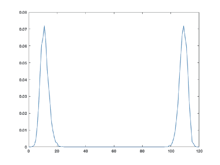
Let . In this case, when conformists are less than of the population, , the corresponding ODE has only one equilibria and it is asymptotically stable . Thus, conformists reach balance as well as the spontaneous class, and hence the entire group reaches balance for large and large . On the other hand, when conformists are more than of the population, , the equilibrium is unstable and the class of conformists reaches dominance of one opinion. In fact, the other two equilibria are and the stability analysis suggests that these equilibrium points are stable. Hence, the model leads to dominance for the whole group. One example is given in Fig. 6 where probabilities are computed using Monte Carlo simulations of trajectories. Here, the total number of agents is with () being the population of the conformists where and spontaneity coefficient .
6 Conclusions
We have proposed a simple binary model where agents hold an opinion from the set at any time . An agent flips his/her opinion based on the opinion distribution of the entire group and his/her personality. We define personality of an agent by a monotonic conformity function and a spontaneity coefficient . When all agents in the group share the same personality, we call the group homogeneous.
Initially, focusing on a homogeneous group, we analyzed the long time probabilities for a large population size for different personality characteristics of the group. The question of what personality characteristics lead to dominance of one opinion was studied. We found that the shape of the conformity function, namely strict convexity or lack thereof, seems to be an important determining factor in whether dominance of one opinion occurs for sufficiently small .
We extended our model to a heterogeneous group, where the group consists of different personality classes. In particular, when the group is formed by two extreme classes, complete conformity and complete spontaneity, the dominance of group opinion is analyzed. In this example, we found that the fraction of the pure conformists was a key determining factor of dominance along with the strict convexity of .
References
- [1] M. Mobilia, A. Petersen, S. Redner, On the role of zealotry in the voter model, Journal of Statistical Mechanics: Theory and Experiment 2007 (08) (2007) P08029.
- [2] P. Nyczka, K. Sznajd-Weron, Anticonformity or independence??insights from statistical physics, Journal of Statistical Physics 151 (1-2) (2013) 174–202.
- [3] S. T. Stamoulas, M. Rathinam, Convergence, stability, and robustness of multidimensional opinion dynamics in continuous time, SIAM Journal on Control and Optimization 56 (3) (2018) 1938–1967.
- [4] V. D. Blondel, J. M. Hendrickx, J. N. Tsitsiklis, Continuous-time average-preserving opinion dynamics with opinion-dependent communications, SIAM Journal on Control and Optimization 48 (8) (2010) 5214–5240.
- [5] F. Ceragioli, P. Frasca, Continuous and discontinuous opinion dynamics with bounded confidence, Nonlinear Analysis: Real World Applications 13 (3) (2012) 1239–1251.
- [6] M. H. DeGroot, Reaching a consensus, Journal of the American Statistical Association 69 (345) (1974) 118–121.
- [7] P. Jia, A. MirTabatabaei, N. E. Friedkin, F. Bullo, Opinion dynamics and the evolution of social power in influence networks, SIAM review 57 (3) (2015) 367–397.
- [8] N. E. Friedkin, E. C. Johnsen, Social influence and opinions, Journal of Mathematical Sociology 15 (3-4) (1990) 193–206.
- [9] M. Bartolozzi, D. B. Leinweber, A. W. Thomas, Stochastic opinion formation in scale-free networks, Physical Review E 72 (4) (2005) 046113.
- [10] J. A. Hołyst, K. Kacperski, F. Schweitzer, Phase transitions in social impact models of opinion formation, Physica A: Statistical Mechanics and its Applications 285 (1) (2000) 199–210.
- [11] E. Yildiz, A. Ozdaglar, D. Acemoglu, A. Saberi, A. Scaglione, Binary opinion dynamics with stubborn agents, ACM Transactions on Economics and Computation 1 (4) (2013) 19.
- [12] K. Sznajd-Weron, J. Sznajd, Opinion evolution in closed community, International Journal of Modern Physics C 11 (06) (2000) 1157–1165.
- [13] M. San Miguel, V. M. Eguiluz, R. Toral, K. Klemm, Binary and multivariate stochastic models of consensus formation, Computing in Science & Engineering 7 (6) (2005) 67–73.
- [14] S. Galam, Modeling the forming of public opinion: an approach from sociophysics, Global Economics and Management Review 18 (1) (2013) 2–11.
- [15] D. H. Zanette, S. Gil, Opinion spreading and agent segregation on evolving networks, Physica D: Nonlinear Phenomena 224 (1-2) (2006) 156–165.
- [16] J. Lyst, K. Kacperski, F. Schweitzer, Social impact models of opinion dynamics, Annual reviews of computational physics 9 (2002) 253–273.
- [17] R. Hegselmann, U. Krause, et al., Opinion dynamics and bounded confidence models, analysis, and simulation, Journal of artificial societies and social simulation 5 (3) (2002).
- [18] G. Weisbuch, G. Deffuant, F. Amblard, J.-P. Nadal, Meet, discuss, and segregate!, Complexity 7 (3) (2002) 55–63.
- [19] T. M. Liggett, et al., Stochastic interacting systems: contact, voter and exclusion processes, Vol. 324, springer science & Business Media, 1999.
- [20] J. J. Schneider, The influence of contrarians and opportunists on the stability of a democracy in the sznajd model, International Journal of Modern Physics C 15 (05) (2004) 659–674.
- [21] K. Sznajd-Weron, M. Tabiszewski, A. M. Timpanaro, Phase transition in the sznajd model with independence, EPL (Europhysics Letters) 96 (4) (2011) 48002.
- [22] M. S. de la Lama, J. M. López, H. S. Wio, Spontaneous emergence of contrarian-like behaviour in an opinion spreading model, EPL (Europhysics Letters) 72 (5) (2005) 851.
- [23] M. A. Javarone, Social influences in opinion dynamics: the role of conformity, Physica A: Statistical Mechanics and its Applications 414 (2014) 19–30.
- [24] N. Khalil, M. San Miguel, R. Toral, Zealots in the mean-field noisy voter model, Physical Review E 97 (1) (2018) 012310.
- [25] S. N. Ethier, T. G. Kurtz, Markov processes: characterization and convergence, Vol. 282, John Wiley & Sons, 2009.
- [26] T. G. Kurtz, Limit theorems and diffusion approximations for density dependent markov chains, in: Stochastic Systems: Modeling, Identification and Optimization, I, Springer, 1976, pp. 67–78.