Conditions for Reionizing the Universe with A Low Galaxy Ionizing Photon Escape FractionJournal: Astrophysical Journal
Abstract
We explore scenarios for reionizing the intergalactic medium with low galaxy ionizing photon escape fractions. We combine simulation-based halo-mass dependent escape fractions with an extrapolation of the observed galaxy rest-ultraviolet luminosity functions to solve for the reionization history from 20 4. We explore the posterior distributions for key unknown quantities, including the limiting halo mass for star-formation, the ionizing photon production efficiency, and a potential contribution from active galactic nuclei (AGN). We marginalize over the allowable parameter space using a Markov Chain Monte Carlo method, finding a solution which satisfies the most model-independent constraints on reionization. Our fiducial model can match observational constraints with an average escape fraction of 5% throughout the bulk of the epoch of reionization if: i) galaxies form stars down to the atomic cooling limit before reionization and a photosuppression mass of log (/M⊙) 9 during/after reionization (13 11); ii) galaxies become more efficient producers of ionizing photons at higher redshifts and fainter magnitudes, and iii) there is a significant, but sub-dominant, contribution by AGN at 7. In this model the faintest galaxies (15) dominate the ionizing emissivity, leading to an earlier start to reionization and a smoother evolution of the ionized volume filling fraction than models which assume a single escape fraction at all redshifts and luminosities. The ionizing emissivity from this model is consistent with observations at 4–5 (and below, when extrapolated), in contrast to some models which assume a single escape fraction. Our predicted ionized volume filling fraction at 7 of 78% ( 8%) is in modest (1–2) tension with observations of Ly emitters at 7 and the damping wing analyses of the two known 7 quasars, which prefer 40–50%.
Keywords:
early universe — galaxies: reionization — galaxies: formation — galaxies: evolutionI Introduction
The reionization of the intergalactic medium (IGM) was the last major phase change in the universe, when high energy ultraviolet (UV) photons from the first luminous sources in the universe ionized hydrogen (and singly ionized helium) in the IGM. Observational constraints on this epoch come from a variety of complementary techniques, and are continuously improving in accuracy and growing in number. Present-day observations constrain the bulk of reionization to be completed by 6 (Fan et al. 2006; McGreer et al. 2015, e.g.,), though some lines of sight may remain somewhat neutral to 5.5 (McGreer et al. 2015; Kulkarni et al. 2018; Pentericci et al. 2018, e.g.,). The beginning of reionization is less well constrained, and depends sensitively on the nature of the ionizing sources. If rare objects such as quasars provide the bulk of the ionizing photons, reionization likely didn’t get well underway until 10 (Madau & Haardt 2015, e.g,). On the other hand, if young, massive stars dominated the ionizing photon budget, reionization may have started much sooner, although the constraints on the electron-scattering optical depth to the cosmic microwave background (CMB) measured by Planck Collaboration et al. 2016b imply that the halfway point came at 8. The apparent dichotomy between the sharp decline in the number density of bright quasars at 2 (Richards et al. 2006; Hopkins et al. 2007, e.g.,) and the relatively shallower decline in the UV luminosity density from galaxies (e.g., Madau & Dickinson 2014, and references therein) has led to the predominant theory that the bulk of the ionizing photon budget came from massive stars.
Better understanding both the temporal and spatial evolution of the process of reionization is key to understanding a variety of unknown physical processes in the early universe, including the time of the onset of the first stars and galaxies, the effects of reionization heating on galaxy formation and growth, and the escape of ionizing photons from galaxies. Present-day efforts to reconstruct the progress of hydrogen reionization involves several major uncertainties around the contribution of both massive stars in galaxies and quasars. Over the past decade advances in the capabilities of near-infrared imaging on the Hubble Space Telescope, necessary to measure rest-frame UV light in the epoch of reionization, have led to robust constraints on the observable non-ionizing UV (1500 Å) luminosity density from galaxies in this epoch.
To understand how these galaxies contribute to reionization, one needs convert this to an ionizing emissivity (; the number of ionizing photons produced per unit time per unit volume which escape the galaxy) as a function of redshift (Finkelstein et al. 2012a; Finkelstein et al. 2015b; Robertson et al. 2013; Robertson et al. 2015; Bouwens et al. 2016b; Bouwens et al. 2015b, e.g.,), which is dependent on three factors: the rest-UV non-ionizing specific luminosity density (), the ionizing photon production efficiency (), and the escape fraction of ionizing photons (). The product of the first two quantities produces the intrinsic ionizing emissivity produced within galaxies (), which when multiplied by produces the escaping ionizing emissivity . This quantity can be used to infer the evolution of the IGM ionized volume filling fraction (denoted as ) by solving a set of ordinary differential equations, which depend on this emissivity, the density of hydrogen, and the recombination time (dependent itself on the clumping factor of the gas and the temperature-dependent recombination coefficient; e.g., Madau et al. 1999; Robertson et al. 2013).
The value of is measured by integrating the observed rest-UV luminosity function to some observationally unknown limiting magnitude. This limiting magnitude is crucial as the steepening faint-end slope with increasing redshift means that the faintest galaxies dominate (Bunker et al. 2004; Yan & Windhorst 2004; Bouwens et al. 2015b; Finkelstein et al. 2015b, e.g.,). Exactly how dominant these faint sources are depends on the shape of the extreme faint-end, which should reverse its steep rise due to stellar feedback, the ability of halos to atomically cool, and Jeans filtering due to the reionization-driven UV background, as shown by a variety of simulations (Bullock et al. 2000; Gnedin 2000; Iliev et al. 2007; Okamoto et al. 2008; Mesinger & Dijkstra 2008; Finlator et al. 2011; Finlator et al. 2012; Alvarez et al. 2012; Oñorbe et al. 2017; Jaacks et al. 2018b, e.g.). Informed by this theoretical work, observational studies have commonly used 13 as this integration limit (Robertson et al. 2015; Finkelstein et al. 2015b, e.g.,).
This limit is 100 fainter than that achievable in even the Hubble Ultra Deep Field (Beckwith et al. 2006) at these redshifts. However, recent observations of much fainter galaxies rendered detectable via gravitational lensing in the Hubble Frontier Fields (Lotz et al. 2017) have begun to provide empirical justification, with evidence that the observed luminosity functions maintain their steep slopes down to 16 at 6 (Atek et al. 2015), and possibly to 15 (Livermore et al. 2017; Bouwens et al. 2017; Atek et al. 2018). We note the concept of a limiting magnitude is an approximation, as the luminosity function should gradually roll over rather then exhibit a steep cut-off (Jaacks et al. 2013; Weisz et al. 2014; Boylan-Kolchin et al. 2015; Jaacks et al. 2018b, e.g.), and any cut-off or turnover point will evolve with redshift as the halo masses evolve, the UV background ramps up, and feedback effects manifest. We refer the reader to the recent review by Dayal & Ferrara 2018 for further discussion on this topic.
The ionizing photon production efficiency converts the (dust-corrected) rest-UV non-ionizing specific luminosity density [erg s-1 Hz-1 Mpc-3] to the intrinsic ionizing emissivity [s-1 Mpc-3]. This efficiency depends on the surface temperatures of the massive stars, which in turn depends on the stellar metallicity, age, and binarity, as well as the initial mass function (Eldridge & Stanway 2009; Stanway et al. 2016; Stanway & Eldridge 2018, e.g.,). If these quantities were known, one could then measure directly. There are however large uncertainties, thus until recently most studies assumed a value of 25.2, expected from modestly metal-poor, but otherwise-normal, single-star population models (Finkelstein et al. 2012a; Robertson et al. 2015, e.g.). This is consistent with the observations that stellar populations in faint 7 galaxies are non-primordial (Finkelstein et al. 2010; Finkelstein et al. 2012b; Wilkins et al. 2011; Bouwens et al. 2012; Bouwens et al. 2014; Dunlop et al. 2013, e.g.,), though it is possible that fainter galaxies have much lower metallicities (Dunlop et al. 2013; Jaacks et al. 2018a).
While full spectroscopic nebular modeling is needed to directly measure , Recent work has shown that the typically assumed conversion from observed non-ionizing to ionizing UV is consistent with the inferred strength of H emission deduced from IRAC photometric colors for bright galaxies at 4 (Bouwens et al. 2016a, e.g.,). However, this same work shows evidence that fainter/bluer galaxies, and galaxies at 5 have higher values of . This implies that may vary both with galaxy luminosity (and/or perhaps halo mass) as well as redshift, consistent with the high values of inferred from the few 7 galaxies with detectable C iii] emission (Stark et al. 2016). This evidence implies that a single value of is not appropriate for all galaxies at all high redshifts.
Finally, to convert the intrinsic ionizing emissivity to that available to ionize the IGM () one needs to assume an escape fraction () for ionizing photons, which is the dominant source of uncertainty. A variety of analyses have shown that when assuming a limiting magnitude of 13 and 25.2, an escape fraction of 10–20% produces the requisite number of ionizing photons to complete reionization by 6 with no contribution from other sources (Finkelstein et al. 2012a; Robertson et al. 2013; Finkelstein et al. 2015b; Robertson et al. 2015; Bouwens et al. 2015a, e.g.,). The assumption of a relatively high escape fraction at 6 is impossible to directly verify, as even a predominantly ionized IGM produces an ionizing optical depth sufficient to absorb all ionizing UV radiation at 4 (Vanzella et al. 2018, e.g.,). (thus unsurprisingly the most distant galaxy with observed ionizing photon escape is at 4.0.)
We must observe galaxies at to directly measure , where there is unambiguous observational evidence that most studied galaxies have low escape fractions (e.g., Siana et al. 2010; Sandberg et al. 2015; Rutkowski et al. 2017; Grazian et al. 2017, though see Steidel et al. 2018). . In particular, studies which stack large samples of star-forming galaxies in deep imaging datasets which probe 912 Å ubiquitously find non-detections, with stringent upper limits of 5%, and sometimes as low as 2% Recent observational programs have improved at identifying galaxies likely to exhibit higher escape fractions, specifically those which exhibit intense ionizing environments as traced by ratios of nebular emission lines, resulting a few dozen direct detections of escaping ionizing photons (Shapley et al. 2016; de Barros et al. 2016; Bian et al. 2017; Vanzella et al. 2018; Izotov et al. 2018, e.g.,). However, the lack of significant ionizing photon escape from the bulk of galaxies strongly implies that the escape fraction from all galaxies at all redshifts cannot be as high as 10–20%.
One way to reconcile this, suggested by a variety of simulations, is if the escape fraction is dependent on the halo mass, where lower-mass halos have higher escape fractions due to lower gas covering fractions and an increased susceptibility of starburst-driven escape routes (Paardekooper et al. 2013; Wise et al. 2014; Paardekooper et al. 2015; Anderson et al. 2017; Xu et al. 2016, e.g.,), while massive halos occasionally exhibit high escape fractions for short periods due to extreme starburst-driven winds clearing channels in the ISM (Paardekooper et al. 2015, e.g.).
In this work, we make use of halo-mass dependent escape fractions predicted from simulations to explore scenarios for completing reionization with low escape fractions for most observable galaxies. In §2, we focus on a critical examination of all assumptions needed to solve for the reionization history, while in §3 we discuss our MCMC framework which we use to probe the full parameter space for all such assumptions, using predominantly model-independant reionization observations to constrain our analysis. These results are given in §4, and discussed in §5. In §6 we explore the implications on the cosmic star-formation rate density to faint luminosities and extremely high redshifts. Throughout this paper, we assume AB magnitudes (Oke & Gunn 1983) and a Planck 2015 cosmology: H0=67.74 km s-1 Mpc-1, 0.309, 0.691, 0.0486 and Y 0.2453 (Planck Collaboration et al. 2016a). We use the variable to denote both halo mass and absolute magnitude, thus we distinguish these by and , respectively.
II Defining the Total Ionizing Emissivity
To model reionization we must calculate the evolution of the ionizing emissivity with redshift, which depends on a number of variables discussed above. Here we attempt to gain new insight into reionization by pairing galaxy observations with simulated, halo-mass dependent escape fractions. As shown in the Appendix, simply replacing a flat 10–20% escape fraction with results from simulations is destined to fail due to the low escape fraction values for all but the smallest halos. We must thus re-examine the assumptions for all critical variables. We allow this by flexibly exploring the dependence of reionization on assumptions about the ionizing photon production efficiency, limiting halo mass for star formation, and a potential contribution from AGN to the ionizing emissivity.
As described in this section, our model includes seven free parameters which, when combined with the observed UV luminosity function, define the emissivity as a function of redshift. In §3 we describe how we constrain the posterior distribution of these parameters within a MCMC framework constrained by several robust observations. We restrict our model to 4, as this more than encompasses the full epoch of hydrogen reionization, and at lower redshifts dusty star-forming galaxies (some of which could be absent from our UV luminosity functions) may contribute to the ionizing photon budget (e.g., Gruppioni et al. 2013; Cowie et al. 2017; Koprowski et al. 2017, though see Casey et al. 2018).
II.1 The Galaxy Ionizing Emissivity
II.1.1 Luminosity Functions
To understand the contribution from galaxies to the ionizing emissivity, we adopt the “reference” luminosity functions of Finkelstein 2016, which were the result of a Markov Chain Monte Carlo (MCMC) Schechter function fit to all recently published data at 4–10. Rather than fitting luminosity functions separately at each redshift, they fit all data simultaneously, solving for the linear relations of the characteristic magnitude M∗(), faint-end slope () and characteristic number density (). To incorporate the uncertainties in these fits into our analysis, we make use of the MCMC chains from F16, using a randomly chosen sample of 104 chain steps (which were verified to be representative of the full chain). We note that while the F16 analysis did not include results from lensed galaxies in the Hubble Frontier Fields, the faint-end slopes used here are consistent with studies of those data, which reach to at 7, finding 2 (Livermore et al. 2017; Bouwens et al. 2017; Atek et al. 2018, e.g.,).
To fully explore the epoch of reionization, it is necessary to extrapolate these results to higher redshift. In our analysis, we consider redshifts from 4 to 20. As the data used to derive these luminosity functions were limited to 10, it is unknown if this extrapolation is valid. Specifically, the faint-end slope is observed to evolve somewhat steeply with redshift (0.11), implying 2.90. While this may be possible (indeed the model results from Mason et al. 2015 find 3.51), it is unknown if this is actually the case. To cover this possibility, in our analysis we consider two scenarios: our fiducial model is one in which the faint-end slope ceases to evolve at 10, and remains at the 10 value of 2.35, while in § IV.2 we also explore the case where continues to steepen at 10. The fiducial luminosity function parameters at the redshifts considered here are given in Table 1, and they are shown in the left panel of Figure 1.
| Redshift | M∗ | log | |
|---|---|---|---|
| (mag) | (Mpc-3) | ||
| 4 | 21.05 | 1.69 | 2.99 |
| 6 | 20.79 | 1.91 | 3.37 |
| 8 | 20.52 | 2.13 | 3.75 |
| 10 | 20.25 | 2.35 | 4.13 |
| 12 | 19.98 | 2.57 | 4.50 |
| 14 | 19.71 | 2.79 | 4.88 |
| 16 | 19.44 | 3.01 | 5.25 |
| 18 | 19.17 | 3.23 | 5.63 |
| 20 | 18.90 | 3.45 | 6.00 |
Note. — The assumed rest-frame UV luminosity functions used in this work, following the evolutionary trend derived via observations as discussed in Finkelstein 2016. Our fiducial model keeps the faint-end slope fixed at 10 to the 10 value of 2.35.
II.1.2 Abundance Matching
As discussed in the following two subsections, we must project the observed UV luminosity function onto the underlying dark matter halo mass function. We use this mapping to obtain both the limiting magnitude and the escape fraction for a given UV luminosity. We follow the abundance matching methods of Behroozi et al. 2013 to map the halo mass to each point on our luminosity functions. Following Finkelstein et al. 2015a, we assume a log-normal UV magnitude scatter at fixed halo mass of 0.2 dex, though we note that a scatter as high as 0.4 dex does not affect the – relation at log (/M⊙) 11. Our derived – relations are shown in the middle panel of Figure 1 for both luminosity function evolution cases we consider.
II.1.3 Minimum Halo Mass for Star Formation
A complete accounting of the available photon budget requires us to include star formation in all galaxies, including those that are too faint to be observed directly. A recent analysis indicates that current observations using lensing at 6 probe galaxies hosted by log(M/M⊙)9.5 halos (Finlator et al. 2016), and theoretical models generally predict that star formation in even lower-mass systems is expected (Paardekooper et al. 2013; Xu et al. 2016, e.g.,). We thus must extrapolate beyond what is observed, yet as This is especially crucial at 6, where observations have shown that the 6 luminosity function has a very steep faint-end slope (Bouwens et al. 2015b; Finkelstein et al. 2015b; Livermore et al. 2017, e.g.,), small changes in the minimum luminosity can have a large impact on the total luminosity density.
Before reionization, Star formation should occur in any halo which can both retain its gas, and cool it to temperatures where it can condense and form stars. Efficient cooling via collisional excitation of H i can occur in galaxies with halo virial temperatures below 104 K. This corresponds to log (/M⊙) 8 at 6 (Okamoto et al. 2008; Finlator et al. 2012), and this critical mass shifts to lower values at higher redshifts, as halos which collapse at earlier times have steeper dark matter potential wells and thus correspondingly higher virial velocities (Barkana & Loeb 2001, e.g.,). Lower mass halos can efficiently cool if they have metals, as predicted by recent simulations which find that significant star formation is happening down to log (/M⊙) 7 at 10–15 due to the availability of metal-line cooling in the immediate aftermath of the formation of Pop III stars (Wise et al. 2014; Xu et al. 2016, e.g.,). Lacking metals, gas can cool inefficiently via molecular hydrogen cooling, which is believed to be the dominant cooling mechanism for the first generation of Population III stars which likely formed in minihalos with log (/M⊙) 7–8 forming at 15–30 (Yoshida et al. 2004; Maio et al. 2010; Johnson et al. 2013; Wise et al. 2014; Jaacks et al. 2018c, e.g.). Due to the inefficiency of this method, Population III stars are not predicted to contribute significantly to the reionizing budget (Ricotti & Ostriker 2004; Greif & Bromm 2006; Ahn et al. 2012; Paardekooper et al. 2013, e.g.,), thus we do not consider star formation in molecular-cooling halos in this work (Jaacks et al. 2018b, though see).
Once the IGM begins to be photo-heated, even atomic cooling halos will begin to have their star formation suppressed. For the lowest mass halos, ionization fronts in reionized regions will suppress star-formation in mini-halos with log (/M⊙) 8 (Shapiro et al. 2004, e.g.,). While more massive halos maybe able to self-shield against this process, gas will not accrete onto dark matter halos with virial temperatures less than the IGM temperature through Jeans filtering. In reionized regions Simulations predict that the halo mass where this process begins to dominate is around log (/M⊙) 9, though the predictions are quite uncertain (Gnedin 2000; Iliev et al. 2007; Mesinger & Dijkstra 2008; Okamoto et al. 2008; Alvarez et al. 2012; Ocvirk et al. 2016; Dawoodbhoy et al. 2018; Ocvirk et al. 2018, e.g.,). Feedback likely also plays a strong role (see Somerville & Davé 2015, and references therein), as these small halos have relatively shallow potential wells, allowing gas to easily be lost. For example, Ceverino et al. 2017 find that stellar feedback causes a flattening in the UV luminosity function at 14, or log (/M⊙) 9.
The physics here are complicated, but in this analysis we wish only to capture the broad trend of an evolving halo mass where star-formation is suppressed. We allow star-formation to occur in halos above the redshift-dependent atomic cooling limit, , which is given by Equation 26 in Barkana & Loeb 2001, assuming a critical virial temperature for atomic cooling of 10,000 K. After reionization begins, we implement photo-suppression below a threshold halo mass due to the rising UV background. However, there are a range of plausible limiting halo masses for this photo-suppression to take effect (Iliev et al. 2007; Mesinger & Dijkstra 2008; Okamoto et al. 2008; Alvarez et al. 2012, e.g.,). In addition, even once gas halts accreting, these galaxies may still form stars for a period of time until they use up all of their previously accreted gas (Sobacchi & Mesinger 2013). We approximate these uncertainties by adding this photo-suppression mass as a free parameter, , with an adopted flat prior of log (⊙) (8.5,10.5) encompassing the range found in the literature. The lower bound was set so that this mass threshold was never lower than the atomic cooling limit at the redshifts considered here; this could have been avoided by allowing the photosuppression mass to be redshift-dependent, but we elected to choose a fixed value in the absence of evidence that this redshift dependance was needed, and to avoid adding another free parameter to our model. The non-ionizing specific UV luminosity density () is calculated at each redshift as the integral of the UV luminosity function down to the magnitude corresponding to this limit, shown in the right-hand panel of Figure 1.for both luminosity function evolution cases we consider. In § III.1 we describe how our model transitions from the atomic cooling limit to the photosuppression mass as reionization progresses.
We reiterate that while our model does not include star-formation beyond the limits specified here, a number of recent simulations show star-formation, especially in the pre-reionization universe, in very low-mass halos of 7 log ⊙ 8. However, modern high-resolution simulations still predict a turnover in the UV luminosity function at magnitudes corresponding to approximately the atomic cooling limit (Wise et al. 2014; Jaacks et al. 2018b, e.g.,). While the flat luminosity function beyond this turnover implies star-formation activity is occurring in lower-mass halos, the shallowing of the luminosity function slope results in these small systems contributing little to the integrated UV luminosity density. As Jaacks et al. 2018b show in their Figure 17, although their UV luminosity function continues to 8, the UV luminosity density asymptotes to a constant value when integrating to 13. Future iterations of our model can better match these theoretical results by including a turnover in our luminosity function, and the results may not be inconsequential as these extreme low-mass halos could have high ionizing photon escape fractions.
II.1.4 Ionizing Photon Production Efficiency
To convert the total non-ionizing ultraviolet luminosity density to the ionizing emissivity, a value for the ionizing photon production efficiency () needs to be assumed. This parameter encompasses all of the physics of the underlying stellar population, many which likely evolve with redshift. For example, the mean metallicity of young stars in galaxies likely decreases from low-to-high redshift, something which has been observationally tracked by a decrease in the typical dust attenuation (Bouwens et al. 2012; Finkelstein et al. 2012b; Bouwens et al. 2014, e.g.,), leading to Lower metallicity stars have hotter stellar photospheres as the metal opacity (mostly due to iron) is lower, and thus a higher ionizing to non-ionizing UV photon ratio. Another factor to be considered is the effect of binary stars. Additionally, recent work on Stellar population synthesis models which include binary stars (Eldridge & Stanway 2009) show that the ionizing flux is boosted by 60% (at low metallicities of 0.3⊙) compared to models with isolated stars only (Stanway et al. 2016) due to both a harder ionizing spectrum from the primary star (which has its envelope stripped), and an increase in mass for the secondary star, allowing more massive stars to exist at later ages.
These effects certainly play a role in high-redshift galaxies, where we cannot directly probe the ionizing flux. However, the production rate of ionizing photons can be inferred their via the detection of nebular emission lines., which, when compared to the observed non-ionizing UV continuum emission, places constraints on . Bouwens et al. 2016a inferred H emission line fluxes from Spitzer/IRAC photometry at 3.8 5.0, finding log 25.34 erg-1 Hz, consistent with typically assumed values of log 25.2–25.3 erg-1 Hz in previous reionization studies (Madau et al. 1999; Kuhlen & Faucher-Giguère 2012; Finkelstein et al. 2012a; Robertson et al. 2015, e.g.,). At 5.1 5.4, Bouwens et al. 2016a found log 25.48 Hz erg-1, hinting at evolution towards larger values at higher redshift, though not at a significant level given the observational uncertainties. Bouwens et al. 2016a also find evidence that the bluest galaxies exhibit even higher values of , with log 25.9 erg-1 Hz for galaxies in their 5.1 5.4 sample with 2.3 (similar results are found for the faintest galaxies in that sample, which, as shown by Bouwens et al. 2014, are likely also the bluest).
Stark et al. 2015a and Stark et al. 2016 measured via ionized carbon emission, finding 25.68 erg-1 Hz in a lensed galaxy at 7.045 with an intrinsic 19.3, and 25.6 for three luminous (22) galaxies at 7.15, 7.48 and 7.73. Further evidence for potential changes in comes from Stark et al. 2015a and Stark et al. 2016, who derive the ionizing environment within galaxies by observing rest-frame UV emission from species of ionized carbon. Stark et al. 2015a detected C iv from a lensed galaxy at 7.045 with an intrinsic 19.3, inferring log 25.68 erg-1 Hz. Stark et al. 2016 published observations of Ly, C iii], and [O iii] (with the latter inferred from Spitzer/IRAC photometry) from three luminous (22) galaxies at 7.15, 7.48 and 7.73. They used photoionization modeling to infer 25.6 for all three galaxies. Lastly, Wilkins et al. 2016b investigated the range of expected from galaxies in the epoch of reionization based on the BlueTides simulation, finding that simulated galaxies spanned the range 25 26, with the highest values obtained when assuming low-metallicity stellar population models which include binaries.
Taken together, this evidence implies that likely depends on redshift and luminosity, which we allow in our model via assuming a fixed value of for galaxies at all redshifts and luminosities is likely not representative of the true ionizing production in distant galaxies. two free parameters, a redshift dependence log and a magnitude dependence log. We assume that at our lowest redshift considered of 4, galaxies brighter than 20 have log 25.34 erg-1 Hz, consistent with the results from Bouwens et al. 2016a for this redshift and luminosity. Galaxies at higher redshifts and/or at fainter luminosities have values of corresponding to
| (1) |
where is the reference magnitude of 20. We assume flat priors on both free parameters of log (0.0,0.4) and log (0.0,0.2). was also constrained to have a maximum value of 26.0, which corresponds to the highest value seen observationally or from simulations (Bouwens et al. 2016a; Wilkins et al. 2016b; Izotov et al. 2017, e.g.,).
II.1.5 Escape Fractions
To derive the ionizing emissivity available to ionize the IGM, we must combine our intrinsic ionizing emissivity () with a model for , which we anchor in the results from the high-resolution First Billion Years (FiBY) simulations. Previous observational studies typically consider only single values, ranging from 10-50% (Finkelstein et al. 2010; Finkelstein et al. 2012a; Robertson et al. 2013; Robertson et al. 2015; Bouwens et al. 2015b; Finkelstein et al. 2015a, e.g.,). However, as discussed in §1, essentially all observations of escaping ionizing radiation from galaxies (albeit at lower redshifts) imply smaller escape fractions. Therefore, rather than assume a single arbitrary value, here we draw on information provided by simulations. While a number of simulations over the past several years have derived this quantity (Razoumov & Sommer-Larsen 2006; Gnedin et al. 2008; Yajima et al. 2011; Kim et al. 2013; Kimm & Cen 2014; Wise et al. 2014, e.g.,), here we use the high-resolution radiative transfer simulations of ionizing photon escape from Paardekooper et al. 2015. These simulations were post-processed on outputs from the FiBY simulation suite which follows the formation of the first stars and galaxies from cosmological initial conditions and leads to a realistic galaxy population at 6 (Khochfar et al in prep). The escape fraction of ionizing photons was determined in more than 75,000 haloes by post-processing the highest resolution FiBY simulations with high-resolution radiative transfer simulations. The radiative transfer simulations were run at the same resolution as the hydrodynamics, allowing the average densities within giant molecular clouds in which stars are born to be resolved. This is essential for the determination of the escape fraction.
Comparing to a number of galaxy properties, this study found that the ionizing escape fraction is strongly anti-correlated with the halo mass. We use their results from all halos that are forming stars, which results in an escape fraction versus halo mass relation which is independant of redshift (we will address photoionization feedback below). At each halo mass (in steps of log[/M⊙] = 0.5) we compute the distribution of the escape fraction via the Kernel Density Estimation (KDE), using cross-validation to compute the optimal KDE bandwidth. We used 20-fold cross-validation, optimizing how well the KDE fits the remaining data. In every step of the cross-validation, the KDE is constructed on 19/20th part of the data, and the log-likelihood of the remaining 1/20th part of the data fitting this KDE is computed. That is done 20 times (every time changing which part of the data is left out) and the result is averaged. This procedure is repeated for different values of the bandwidth and the bandwidth with the best score has been chosen. While a larger bandwidth would result in a smoother distribution, it would not fit the edges of the distribution as well as our adopted bandwidth. Our adopted escape fraction distributions are shown in Figure 2. These escape fractions are effectively time-averaged, as the distributions shown are the average of the instantaneous escape fractions of every halo in the simulation. This figure highlights that the escape fraction distributions are quite broad, but only halos with log(/M⊙) 8.5 have more than half of their distribution at 1%.
At log(/M⊙) 9 there is a small probability that 10%; these few halos are undergoing an extreme starburst and the supernova feedback is able to evacuate almost all of the gas. As the simulation does not have a representative sample of halos with log(/M⊙) 9.5, we assume that halos with log(/M⊙) 11 have 0, and that halos with log(/M⊙) 9-11 have a similar distribution as those at halos with log(/M⊙) 9 but without the small peak at high (due to the increased potential making it more difficult for supernovae to remove all the gas), as shown by the gray dashed line in Figure 2. We note that if we had treated halos with log(/M⊙) 11 the same as those with log(/M⊙) 10, we find almost no differences in the resulting ionization history (completing at 5.7, compared to 5.5 for our fiducial model), although in the post-reionization universe the galaxy emissivity drops off slightly more shallowly, with a corresponding slight decrease in the needed AGN emissivity (§2.2).
The normalization of the escape fraction may be inaccurate in the Paardekooper et al. 2015 simulations for several reasons. The resolution of the simulations is insufficient to resolve the birth cloud of the star particles in great detail, potentially missing physics on the scale of individual stars that can affect the escape fraction. Simulations have shown that better resolving the ISM around the stars results in a higher escape fraction because the porosity of the gas is better accounted for (Paardekooper et al. 2011). In addition, the stellar population model in their simulations does not include the effects of binary interaction, such as mass transfer between stars and mergers of binaries. These processes have been shown to affect the average escape fraction in a halo because massive stars in binaries live longer, and thus emit many ionizing photons when the birth cloud of the stars has been dissolved by supernova explosions of the single massive stars in the population (Ma et al. 2016).
We thus adopt an escape fraction “scale factor”, where in a given iteration of our model, the escape fractions at all halo masses are scaled by the same factor, preserving the halo-mass-dependence of the escape fraction. We do not allow this scale factor to vary with redshift, as the simulations find roughly constant escape fractions at fixed halo mass through the epoch 6 15, and the expected physical reasons for this scale factor do not depend on redshift. We denote this parameter below as , and adopt a flat prior on over the range (0,10).
The total ionizing emissivity from galaxies is thus calculated as , where the latter term includes this scale factor.
II.2 Inclusion of an Active Galactic Nuclei Contribution
While quasars have been disfavored as the dominant source of the reionization ionizing photon budget (Shapiro & Giroux 1987, e.g.,), the low observed galaxy escape fractions leave room for some contribution from active galactic nuclei. This is not in violation of previous results, as most observations at 4 probe the bright end of the AGN luminosity function (e.g., quasars only), thus, similar to galaxies, it may be that the AGN luminosity function has a steepening faint end slope, and that faint AGNs, and not the rare quasars, are significant contributors. once quasars were a common inclusion when considering sources of ionizing photons for reionization, the relative paucity of quasars at 4 found by SDSS, combined with the observed steepening of the star-forming galaxy luminosity function faint-end slope, has led many to conclude that quasars were not significant contributors. However,
There is observational evidence in favor of this possibility, as Giallongo et al. 2015 discovered faint AGNs at 4–6 by searching the positions of known galaxies at those epochs in deep Chandra X-ray data in the GOODS-S field. At 4, Giallongo et al. found ionizing emissivities nearly an order of magnitude greater than those implied by the bolometric quasar luminosity function work of Hopkins et al. 2007, and a factor of a few higher than Glikman et al. 2011, with the evolution to 5–6 shallower than that of Hopkins et al. 2007. Taken at face value, ionizing photons generated from AGN could account for the entire reionization photon budget, with no contribution from galaxies at all (Madau & Haardt 2015). They found 22 AGN candidates, probing several magnitudes fainter on the AGN luminosity function than previous studies which rely on discovering sources in the X-ray images. This led to a followup analysis by Madau & Haardt 2015, who showed that if the Giallongo et al. results were taken at face value, The Giallongo et al. results have been met with some skepticism over the photometric redshifts of the sources (Parsa et al. 2018, e.g.,), and also the apparent lower emissivity at similar redshifts (McGreer et al. 2018, e.g.,). Additionally, Giallongo et al. note that they cannot rule out a significant stellar contribution to the X-ray luminosity. However, given the difficulties in isolating faint AGN at high redshift (Stevans et al. 2018, e.g.,), and the fact that current observations span a large range at 4, we allow a contribution from AGN to the ionizing budget in our fiducial model. Figure 3 shows the inferred evolution of the AGN comoving ionizing emissivity both from the previous work by Hopkins et al. 2007, and the “quasars can do it all” recent work by Madau & Haardt 2015, along with a number of observational results from the literature.

Our initial emissivity matches Madau & Haardt 2015 at 2.5, and at higher redshifts is a simple exponential with a slope constrained to be between those of Hopkins et al. 2007 at the low end, and Madau & Haardt 2015 at the high end, spanning the full range of observational results. Our emissivity is governed by three free parameters: a scale factor (0,1) applied to the emissivity allowing it to be lower than initially assumed (due to a range of physical effects, including a non-unity AGN ionizing photon escape fraction, which is likely the case for less-luminous AGNs; Trebitsch et al. 2018); a redshift-evolution exponential slope (1.05,0.34), which approximately reproduces the Hopkins et al. 2007 and Madau & Haardt 2015 respective AGN ionizing emissivity evolution in this formalism; and a maximum redshift , above which the AGN ionizing emissivity is assumed to be zero. The functional form for our monochromatic 912 Å emissivity is given by
| (2) |
where the first exponential term is the initial emissivity, and the term in parentheses is a normalization factor, normalizing our emissivity (prior to the application of a scale factor) to be equal to that of Madau & Haardt 2015 at 2.5 (whose functional form is given in the numerator). We note that while this emissivity is included in our analysis, it is allowed within our formalism to be negligibly low in the epoch of reionization, thus we are not “forcing” AGNs to contribute significantly. We discuss our fiducial results in §4, but they are shown in Figure 3, falling roughly in the middle of the allowed range.
The total emissivity from our model at a given redshift is the sum of that from galaxies (§ II.1) and AGN: .
| Parameter Name | Initialization | Initialization | Flat prior | Posterior |
|---|---|---|---|---|
| Central Value | constraints | Median (68% Confidence) | ||
| fesc,scalea | 5.0 | 1.0 | 0, 10 | 5.2 (3.3 to 7.5) |
| log (Mh,supp/M⊙)b | 9.0 | 0.5 | 8.5, 10.5 | 8.9 (9.5) |
| log | 0.10 | 0.05 | 0, 0.4 | 0.13 (0.05 to 0.25) |
| log | 0.05 | 0.03 | 0, 0.2 | 0.07 (0.03 to 0.13) |
| AGNscalee | 0.8 | 0.2 | 0, 1 | 0.77 (0.47) |
| g | 10.0 | 2.0 | 4, 12 | 9.2 (6.9) |
| AGNslopef | 0.5 | 0.3 | 1.2, 0.1 | 0.39 (0.93) |
Note. — The free parameters for our fiducial model. The initialization central value and initialization define a normal distribution from which each walker draws an initial value. a The scale factor applied to the halo-mass-dependent escape fractions from the Paardekooper et al. 2015 simulations. b Post-reionization photosuppression halo mass. c Evolution of ionizing photon production efficiency with redshift and dabsolute magnitude. eScale factor applied to the AGN emissivity (mimicking an AGN ionizing photon escape fraction). f Exponential slope of the AGN emissivity with redshift, constrained to be zero at some gmaximum redshift. The last column gives the median of the posterior distribution, and the central 68% confidence range (or upper/lower 84% confidence limits when the distribution is one-sided).
II.3 Calculating
We calculate the IGM volume ionized fraction by solving the differential equation
| (3) |
where is the comoving ionizing emissivity derived above, is the comoving hydrogen density, and is the IGM hydrogen recombination time. The comoving hydrogen density is calculated as the product of the hydrogen mass fraction (defined as , where is the helium mass fraction), the dimensionless cosmic baryon density , and the critical density (defined as 3/8). The IGM recombination time is given by
| (4) |
where is the temperature-dependent case B recombination coefficient for hydrogen using the functional form given by Hui & Gnedin 1997. Following Robertson et al. 2015, we evaluate this at 20,000 K (had we assumed 15,000 K, would be higher by a factor of 1.29). We assume a redshift-dependent hydrogen clumping factor from the simulations of Pawlik et al. 2015, which evolves from 4.8 at 6, to =1.5 at 14. We solve for by integrating the ordinary differential equation in Equation 1 using the IDL routine from 20 to 4.
III Exploring the Full Reionization Parameter Space with MCMC
Using the set of seven free parameters defined in §2 our model can describe the escaping ionizing emissivity from both star-forming galaxies and super-massive black hole accretion (AGN) activity. In this section we describe how we use a MCMC framework to derive the posteriors on these free parameters using a set of robust observational constraints. We used an IDL implementation of the affine-invariant sampler (Goodman & Weare 2010) to sample the posterior, which is similar in production to the Python emcee package (Foreman-Mackey et al. 2013). We used the recommended stretch parameter of with 1000 walkers. Each walker was initialized by choosing a starting position for each of the free parameters, randomly drawn from a normal distribution with a central value and width given in Table 2. We assumed a flat prior on each of our seven free parameters, with the prior bounds also listed in Table 2. If the log likelihood of a given set of parameters was not finite (i.e., it violated the parameter flat priors), a new set of parameters was drawn, until a set which gave a finite probability was drawn to initialize each of the 1000 walkers. The exact initialization values are not crucial as the burn-in process ensures that the starting positions do not affect the results.
III.1 Method
In this sub-section we describe in detail our MCMC analysis. A flowchart of this procedure is shown in Figure 4. In each step of the chain, our routine used the chosen set of seven free parameters to complete the following calculations:
- 1.
For each redshift interval of =0.1 from 4 to 20, we use a randomly drawn set of Schechter function parameters from the available F16 MCMC chains, where the drawn parameters are the redshift-evolution terms , , and . We use these parameterizations to calculate the non-ionizing specific UV luminosity density in absolute magnitude bin intervals of =0.1 from 6 to 24. These were then corrected for dust attenuation () using the method described in Finkelstein (2016), which uses the relation between and from Bouwens et al. 2014, the relation between and AUV from Meurer et al. 1999, and the dust attenuation curve from Calzetti et al. 2000. A scatter in at fixed of 0.35 was assumed, and zero dust attenuation was assumed at 9 (Bouwens et al. 2014; Wilkins et al. 2016a). We note that given the halo mass dependency of the escape fractions the bulk of ionizing photons come from faint galaxies with minimal dust, thus our final results are not sensitive to this correction. To validate this, we performed a model run with no dust correction, and found no significant change in the evolution of the ionization history.
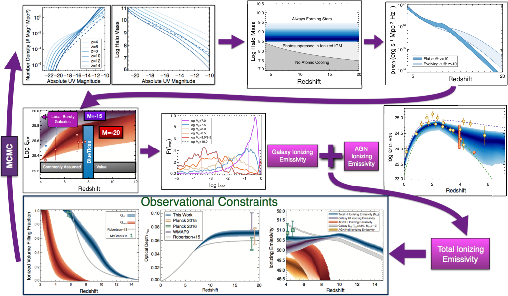
Figure 4: A visual description of our Markov Chain Monte Carlo procedure for constraining the posteriors on our free parameters, described in full in § III.1. All figures appear full-size elsewhere in the paper. - 2.
The intrinsic ionizing emissivity was calculated by multiplying by the appropriate value of for the values of log and log in a given step. The escaping ionizing emissivity was then calculated as multiplied by the escape fraction, where the escape fraction is randomly drawn in each step of the chain for each absolute magnitude interval, from the probability distribution function (PDF) corresponding to the halo mass for the given absolute magnitude (from the – relations described above). One feature of our process is that by randomly sampling these PDFs over many MCMC chain steps, we marginalize over the distribution of possible escape fractions, such that this scatter is encompassed in our final results.
- 3.
The IGM volume ionized fraction of hydrogen was calculated following § II.3. While solving the differential equation, we emulated the effects of photosuppression by calculating the emissivity down to the limiting UV magnitude corresponding to both the atomic cooling limit at a given redshift (; applicable for neutral regions), and also to for the given chain step (; for ionized regions). The total value of for each redshift bin was then calculated as
(5) where the first term accounts for ionizing photons from all galaxies above the photosuppression limit, while the second term accounts for those photons from halos between the photosuppression limit and the atomic cooling limit, but only in the fraction of the volume which is still neutral at a given redshift. We note that this is an approximation as we can only track the globally-averaged ionized fraction, and thus it does not account for the effects of spatial clustering of halos on the ionized fraction in their proximity (e.g., the topology of reionization). The total ionizing emissivity was then calculated as that from galaxies combined with that from AGN, , where the latter was calculated from as described in § II.2, assuming an AGN H I ionizing spectral index of 1.7 (Lusso et al. 2015).
- 4.
While helium becomes singly ionized at a similar energy as hydrogen, high-energy photons from AGN can doubly-ionize helium. We thus calculate the emissivity of He ii ionizing photons (energies 4 Ryd) again assuming a spectral index of 1.7, and solve for the IGM volume ionized fraction of He iii using
(6) and
(7) The volume ionized fraction of He ii was then assumed to be . We assume (see § V.3.2 for discussion).
- 5.
Using the calculated volume ionized fractions for H ii, He ii, and He iii, we calculated the electron scattering optical depth as measured from the CMB as
(8) with
(9) integrated from 0 to 20.
III.2 Observational Constraints
The outcomes of these calculations are the volume ionized fractions of H i, He i and He ii, the galaxy and AGN ionizing emissivities, and the electron scattering optical depth, all as a function of redshift. To calculate the likelihood for our model and constrain our free parameters, we used the following observations:
- 1.
The integrated hydrogen ionizing emissivity at 4.0 and 4.75 from Becker & Bolton 2013, synthesized from a variety of measurements of the IGM based on spectroscopy of high-redshift quasars. They find that this quantity rises from 3.2 to 4.75, which is consistent with the idea that a steepening galaxy UV luminosity function faint-end slope results in more ionizing photons at higher redshifts. We use their measurements of log 0.139 photons s-1 Mpc-3 at 4.0 and log 0.014 photons s-1 Mpc-3 at 4.75. These uncertainties include both the statistical errors, and the much larger systematic errors. We did not use measurements at 4, as our luminosity functions were calculated only at 4. We also did not include the upper limit on the integrated emissivity at 6 from Bolton & Haehnelt 2007, as the value of log (0.585 was derived assuming that the ionizing background is uniform, while recent measurements imply that there are substantial spatial variations (Fan et al. 2006; Becker et al. 2015; Bosman et al. 2018; Becker et al. 2018, e.g.,). Future results taking advantage of updated measurements of the spatial inhomogeneities in the ionizing background, the IGM temperature, and the mean free path of ionizing photons will both decrease these systematic uncertainties, and allow more robust results at higher redshifts, further constraining models such as the one we present here. For each step in our chain, we calculated the goodness-of-fit statistic between both the 4 and 4.75 observations and the summed galaxy and AGN ionizing emissivity from our model.
Figure 5: Each panel shows the smoothed posterior distribution for each of our modeled free parameters. The different colored lines denote which steps out of our 100,000-step chain were used (denoted by the legend in the lower-right). As these distributions do not appear to significantly change after Step #70,000, we adopt as our fiducial posteriors that from the last 5,000 steps of the chain (corresponding to the last 5%), denoted by the black line. We performed the Gelman-Rubin test, which showed that this model is highly converged. The majority of these parameters have a relatively broad posterior distribution, which is propagated forward into the uncertainties in our reionization model. More robust observational constraints are needed if we wish to further constrain these parameters. - 2.
The electron scattering optical depth to the CMB (). This quantity measures the integrated optical depth of Thomson scattering to the CMB. This scattering is caused by the interaction of CMB photons with free electrons as they travel from the surface of last scattering to the present day, and thus it possesses constraining power on models of reionization. Models which reionize earlier will have correspondingly higher values of , and vice versa. Assuming that reionization happens instantaneously, can be converted into a “reionization redshift” (). While most models predict reionization to be spatially and temporally inhomogeneous, this redshift is still a useful indicator of a rough midway point for the reionization process. The first measurements of from the Wilkinson Microwave Anisotropy Probe (WMAP) Year 1 results showed 0.170.06, which suggested an instantaneous “reionization redshift” of 175 (Spergel et al. 2003). Additional data from WMAP revised these estimates immediately downward, from the WMAP Year 3 result of 0.0880.03 (Spergel et al. 2007) to the final WMAP Year 9 result of 0.0880.013 (Hinshaw et al. 2013), and 10.51.1. The advent of the Planck satellite has revised these estimates again downward to 0.0660.012 and 8.81.1 (Planck Collaboration et al. 2016a). Given the relatively large uncertainties of both the WMAP 9 and Planck measures, the discrepancy is only significant at the 1.3 level. However, even more recent 2016 results have been published, highlighting improved removal of systematics from the Planck high-frequency data, showing 0.0550.009 (Planck Collaboration et al. 2016b), discrepant from the WMAP9 data at 2.1 significance.
We elect use this newer 2016 Planck value of as our fiducial constraint. When comparing to R15, it is important to remember that they used the 2015 value, though we note that the 2015 and 2016 Planck values differ only at the 0.7 level. For each step in our chain, we computed between the observational value of and that calculated from our model given in Equation 8, which includes the contribution to both from ionizing hydrogen, and singly and doubly ionized helium. In § IV.1.5 we explore how our results change if we use the lower 2016 value.
- 3.
The model-independent lower limits on the IGM ionized fraction of Q(1) at 5.9, and Q (1) at 5.6 from McGreer et al. 2015. This study measured the fraction of “dark” pixels in the Ly and Ly forests of a sample of 22 bright quasars at 5.7 – 6.4. Regions of the IGM containing any pre-reionization neutral hydrogen should result in completely saturated absorption in both of these transitions. This method only provides a lower limit, as some absorption may also be due to collapsed systems, or residual H i in ionized gas. However, it is model independent as it does not depend on the intrinsic quasar spectral shape (McGreer et al. 2015, see discussion in). Finally, as this method combines several objects (and, several locations along the line-of-sight to each object), it is far more robust against cosmic variance, and uncertainties due to inhomogeneous reionization than neutral fractions derived via effective optical depths to single quasars (Fan et al. 2006; Bolton et al. 2011; Greig et al. 2017; Bañados et al. 2018, e.g.,).
For each step in our chain, we calculated the goodness-of-fit statistic between the ionized fraction in our model at each of these two redshifts, and these measurements. As these are one-sided lower limits on the ionized fraction, if the model value was above these measurements ( 0.94, 0.96 at 5.9, 5.6), was set to zero; if the model was below these values, was calculated in the usual way using the published uncertainties in each redshift bin.
Lastly, to rule out models where reionization ends too late, we added a conservative effective prior that H i reionization must be complete by 5. While the McGreer et al. 2015 measurements suggest it is nearly completed by 6, observations by Becker et al. 2015 have shown significant line-of-sight variation in Ly forest transmission measurements, implying significant UV background fluctuations at 5.6 – 6 (Becker et al. 2018). However, they find that by 5, the data are consistent with reionization being fully completed. Therefore, models which have 1.0 at 5 have , and are rejected.
III.3 Deriving Posteriors
Rather than choose a pre-defined number of steps for the burn-in period, we elected to run our chain for 105 steps, and then examine the results to explore where the chain has converged, and select a final set of samples to derive the posteriors. In Figure 5 we show the distributions of each of our seven free parameters for different groupings of 104 steps. One can see that over the first few iterations of 104 steps, the parameter distributions change, but that after 7 104 steps the changes begin to stabilize, such that the distributions only exhibit minor changes towards the end of the chain. For this reason, we defined the last 5000 steps of the chain as those used to sample the posterior distribution of our free parameters.
The acceptance fraction for this fiducial model was 14.5%. We also ran this model ten independant times to check for convergence, finding that the acceptances fractions spanned 14.1% – 14.6%. We tested for convergence by comparing the posterior distributions of our free parameters using the Gelman-Rubin test. Specifically, we used the IDL routine, which computes the Gelman-Rubin statistic. We found 1.00 for all seven of our free parameters (from 1.00007 for , to 1.0060 for ), showing that this model is highly converged.
When we compare versions of our model, we use the Deviance Information Criteria (DIC; rather than the full Bayes factors, which are prohibitive to compute for our high-dimensional parameter space). This is similar to the Bayesian Information criteria (Liddle 2004) in that it takes into account both the number of data points and the number of free parameters. However, the DIC makes use of the full chain, rather than just the median values. The DIC is defined as , where is the value of of our model using the median of the posterior chains for each parameter, and is defined as , where N is the number of samples in the posterior (5000 here), and is the sample index. is thus twice the difference between and the average value of for the full chain. For a model to be preferred over a competing model, it must have a lower DIC, with the significance of the result determined qualitatively by the “Jeffreys Scale”. Here we make use of the updated interpretation by Kass & Raftery 1995, where DIC 2/6/10 is positive/strong/decisive evidence against the model with the larger value of DIC.
As the MCMC fitting routine did not save the results of the model, such as , or , it was necessary to recompute those after completion of the chain for further analysis and plotting. This was done initially using the final 10,000 steps, calculating everything in an identical manner as was done in the chain. We use this larger number as the random draw process of our escape fraction parameterization causes the results of these re-calculations to occasionally differ slightly than those from the MCMC process, which can result in a particular parameter set violating the prior of reionization completion by 5 (20% of the trials for our fiducial set, but 40% for a run with minimal AGN contribution at 6; see § V.3.3). For this reason, we use a randomly-selected 5000 of these final 10,000 steps which do not violate the prior to calculate the distributions of , or . We note that we have run these calculations several times, and differences in the results from run-to-run are negligible due to the large number of samples.
IV Results
IV.1 Fiducial Model
IV.1.1 Posterior Distributions of Free Parameters
The black lines in Figure 5 show the posterior distributions of our free parameters for our fiducial model. The median values and 68% confidence ranges are listed in Table 2, and we show the covariances between our model parameters as a triangle plot in Figure 6. Of these seven distributions, three have a clearly defined peak in the posterior distribution within our prior range. The parameter fesc,scale prefers a value near 5, with a 68% confidence range of 3.3 fesc,scale 7.5. This implies that our model best matches observations when the escape fractions from the simulations are scaled up by a factor of 3–8. As discussed in § II.1.5, this up-scaling is not surprising, as the simulations were unable to resolve the birth cloud of the star particles, and so the porosity of the gas may be underestimated (though see also Gnedin & Kaurov 2014, who invoke a sub-unity scale factor to account for unresolved systems providing excess absorption). In § V.2 we will discuss the implications of this up-scaling for the average galaxy escape fraction, and its evolution with redshift.
The parameters related to also show a clear peak, with log 0.13, and log 0.07, albeit with broad tails to higher values. These results indicate that, under our model, galaxies must have higher ionizing photon production efficiencies both at higher redshifts, and at lower luminosities. These results are broadly consistent with both the scarce observations at high redshift, but also observations from local analogs for high-redshift galaxies, which we discuss in § V.5.
The remaining four parameters had more one-sided distributions. The filtering mass has a clear preference for the lower end of our allowed range, with a 1-sided 84% upper limit of log (/M⊙) 9.5. This indicates that the model requires star-formation in halos as small as possible for as long as possible. We note that our prior of log (/M⊙) 8.5 was set so that the filtering mass did not drop below the atomic cooling mass throughout our redshift range. It is plausible that if we reduced this prior our model would prefer even lower values, though, as discussed below in §V.4, lower values would be in greater conflict with previous simulation work on the post-UV background filtering mass.
The final three parameters govern the AGN contribution. Combined, they prefer an AGN contribution which evolves relatively shallowly downward with increasing redshift (though not as shallowly as the Madau & Haardt 2015 model), with AGNs present to as high a redshift as allowed, and with a high escape fraction for ionizing photons produced by AGNs. In §V.3.1, we compare the resultant emissivity from these combined parameters to previous observations. The posterior results from this fiducial model corresponds to a DIC value of 5.3.
IV.1.2 Comparison with Constraints
Figure 7 shows the distribution of both and for our fiducial model. The blue-shaded region shows the 68% confidence range on our evolution of . This result is consistent with the observations from McGreer et al. 2015 used to constrain our model, as the lower 68% of our results fall near the lower 68% confidence on their lower limits at 5.6 and 5.9. Our model achieves 1 by 5.6 0.5. Although previous studies have adopted a prior that reionization ended by , it is plausible that reionization ended later. Indeed, significant neutral patches may be necessary to explain the most opaque stretches of the Ly forest at – in particular, the comoving Mpc Ly trough observed by Becker et al. 2015 (Kulkarni et al. 2018).

The shape of the evolution of from our fiducial model shows a roughly linear evolution with redshift from 6 to 10, with a slight acceleration in the evolution at 10 as the faint-end slope of the galaxy luminosity function in our fiducial model stops evolving. This evolution is in sharp contrast to the results of Robertson et al. (2015), which imply that reionization starts very slowly at 10, and then undergoes a rapid acceleration at 10. This stark difference can be understood by the differences in these two models. The R15 model fits a variable star-formation rate (SFR) density to the observations of the galaxy UV luminosity function from a variety of sources, and uses as an additional constraint the 2015 value of the Planck optical depth. They convert their derived SFR density to an ionizing emissivity by assuming a single value for the escape fraction (20%) and ionizing photon production efficiency (log[] 53.14 Lyc photons s-1 M⊙-1 yr-1; 25.24 in the units used here of Hz erg-1). These assumed values are comparable to those used for the purple shaded region in Figure 21 in the Appendix (=13%; log[] 25.34), which give near-identical results to those from Robertson et al. when using our assumed luminosity functions, highlighting that the minor differences in the luminosity functions assumed (or resultant SFR density) do not play a large role in the differences in .
The differences in and must therefore be responsible. While both certainly play a role, the differences in are easy to understand when simply exploring . In the Robertson et al. model, galaxies at all redshifts and luminosities have the same escape fraction of 20%. This means that the ionizing emissivity from a given luminosity range is directly proportional to the non-ionizing UV luminosity density in that same range. The result of this assumption is that the faintest galaxies (14; at 6) do not play a major role. This is illustrated in Figure 8, where the gray shaded lines show the cumulative ionizing emissivity using the assumptions from Robertson et al (albeit with our luminosity functions used here; as discussed in the preceding paragraph, this results in minimal differences). At 6, at the end of reionization, half of the ionizing emissivity comes from rather bright galaxies, with L 0.1L∗ in the Robertson et al. model. While the evolving faint end slope changes this with redshift, even by 10, a near majority of the ionizing emissivity comes from galaxies with L 0.01L∗. As massive/bright galaxies are building up with time, the relative insignificance of L 0.01L∗ galaxies to the ionizing photon budget means that reionization gets a late start. As the brighter/more massive galaxies build up, the ionizing emissivity increases rapidly, resulting in a reionization history that starts late, but finishes quickly.
The blue shaded lines in Figure 8 show the results of our fiducial model. While the same luminosity functions are assumed as the gray lines, in our model the escape fraction is halo-mass dependent, so even modestly-bright galaxies contribute very little, while the faintest galaxies dominate. This, combined with the steepening faint-end slope at higher redshift, allows reionization to begin earlier. This difference is enhanced by our evolution in to higher values at higher redshifts and lower luminosities, allowing those galaxies which have significant escape fractions to have larger ionizing photon budgets. However, as the faint-end slope shallows with decreasing redshift, the emissivity from galaxies from our model decreases, resulting in a very constrained ionizing photon budget towards the end of reionization, discussed in § IV.1.4.
While both models can successfully complete reionization, the different assumptions on the escape fraction result in modest differences in the reionization history. These differences are greatest at 9 where the Robertson et al. model, driven by modestly bright galaxies, predicts 0.2, and our model, driven by the faintest galaxies, predicts 0.5. Future observations may be able to distinguish between these scenarios, and can thus potentially constrain the luminosity range of the galaxies driving reionization. In § V.1 and Figure 11 we further compare our results for to several observational and theoretical results in the literature.


IV.1.3 He II Reionization
While we did not include any constraints on the ionization of He ii in our model, here we comment on the resultant distribution of , shown as the red-shaded region in Figure 7. Our fiducial model results in a He ii reionization history which gets started at a low level at 6, as the AGN help to complete hydrogen reionization. The volume ionized fraction of He iii hits 50% at 3.4 0.6, and He ii reionization completes at 2.7 0.4. This is consistent with observations of the H i and He ii Ly forests. Current observations of the latter show a strong evolution in its mean opacity and dispersion at (Worseck et al. 2011; Worseck et al. 2016a, e.g.). Additionally, the analogue of Gunn-Peterson troughs observed in the He ii Ly forest have been used to place limits of at the cosmic mean density, which implies that He ii reionization was likely still in progress at (McQuinn 2009; Shull et al. 2010; Syphers & Shull 2014). Finally, recent H i Ly forest measurements have found evidence for a bump in the thermal history of the IGM at , which has been interpreted to coincide with the end of the He ii reionization process (Schaye et al. 2000; Becker et al. 2011; Hiss et al. 2017; Puchwein et al. 2015; Upton Sanderbeck et al. 2016, e.g.).
Together, these measurements provide evidence that He ii reionization may be ending at , consistent with our findings (see however McQuinn & Worseck 2014; Davies & Furlanetto 2014; Davies et al. 2017, for alternative interpretations of the He ii Ly forest data). We note that our results also suggest a more extended He ii reionization process than is found in existing simulations – with a 1 upper bound of as much as complete by (McQuinn et al. 2009; Compostella et al. 2013; La Plante et al. 2017). This is qualitatively consistent with the conclusion of Worseck et al. 2016a, who find evidence for extended reionization in the statistics of the He ii Ly forest opacity11 1 See however D’Aloisio et al. 2017 for a discussion of potential caveats in simulating the impact of He ii reionization on the transmission statistics of the He ii Ly forest..
IV.1.4 Comparison with Constraints
In the left panel of Figure 9 we show the evolution of the ionizing emissivity. The blue-shaded region denotes the total H i ionizing emissivity, which is consistent with the observational constraints used for our model. Notably, the emissivity in our model exhibits a slight rise from 4 to 10, consistent with the observations from Becker & Bolton 2013 of an increasing emissivity from 2 to 5. The purple and red shaded regions denote the components of this emissivity contributed by galaxies and AGN, respectively. Although the non-ionizing emissivity from galaxies increases with decreasing redshift from 10 to 4 (Figure 1), the ionizing emissivity does the opposite. This is due to a combination of the faint-end slope of the UV luminosity function becoming shallower, resulting in less luminosity coming from faint galaxies, while it is those very faint galaxies which have the highest escape fractions. This can be better understood by examining Figure 8. While the cumulative ionizing emissivity at 4 is not highly dissimilar to that at 10, Figure 1 highlights that the 10 universe harbors a greater abundance of extremely faint (15) galaxies than the 4 universe. These factors combine to create a galaxy ionizing emissivity which counterintuitively increases with increasing redshift at 10. This emissivity peaks at 10, and then procedes to decline to higher redshift. This transition point is set by the assumption in our fiducial model that the faint-end slope does not get any steeper at 10, while and continue to decline to higher redshifts, lowering the overall emissivity.
The gray curve shows the emissivity if one assumed a fixed limiting magnitude of 13 and escape fraction of 13%. The difference in the ionization history from our model and that from previous results (Robertson et al. 2015; Finkelstein et al. 2015b, e.g.) can be understood by comparing this to the blue curve. Our model has a greater emissivity at 9, allowing an earlier start to reionization. The emissivity at 7 flattens out – just enough to complete reionization by 5.6, but not enough to exceed the emissivity observations at lower redshifts. We note that this gray curve, when extrapolated to 4, will exceed the emissivity measurements from Becker & Bolton 2013. This indicates that some previous models with fixed large escape fractions may have not matched all observational data when considering 6 (Stanway et al. 2016, see also).
The AGN emissivity, shown by the red shaded region, increases with decreasing redshift. This is by construction as our method assumes an AGN emissivity which rises with decreasing redshift, although the exact slope of this increase and the normalization are set by the posterior distributions of these two free parameters. The AGN emissivity, and specifically how it compares to that from galaxies, is discussed further in § V.3.1 below.
IV.1.5 Comparison with Constraints
The right panel of Figure 9 shows the posterior distribution on from our fiducial model. The median value from our model is 0.071 0.005 (integrated to 20).
This is higher than the recent 2016 value published by the Planck collaboration of 0.055 0.009, which we used as our constraint. However, the tension is not high, with the difference being significant at only the 1.55 level (we note that our result is 0.4 higher than the 2015 Planck value of 0.066 0.012, and 1.2 lower than the final WMAP9 value of 0.088 0.013). Comparing to R15 (who used the 2015 Planck value), while our model prefers an earlier start to reionization, the large uncertainties on result in both our model and the results from R15 maintaining consistency with the observational constraints.

Lowering would require removing electrons somewhere along the line-of-sight. One could do this by, for example, slightly lowering the galaxy emissivities, resulting in a slightly later end to reionization. However, the emissivities from the model are already at the lower-end of the observations, and the ionization history is also pushing the limits of the observations. Thus, while this would decrease the tension between the model and the observations, it would increase the tension on our other two constraints. Clearly reduced observational uncertainties on will help, though the outlook for significant future improvement is uncertain. We present tabulated values of the results from this fiducial model in Table 3. As listed in the table, the ratio of the galaxy-to-AGN ionizing emissivity becomes infinite at redshifts when there is no AGN contribution.
IV.2 Evolving Versus Flat Faint-End Slope
Our model uses a redshift-dependent parameterization of the UV luminosity function, which stipulates that the characteristic luminosity and number density decrease to increasing redshift, while the faint-end slope becomes steeper. While these parameterizations were developed by fitting to the observational data at 410, in our model we extrapolate to higher redshift. As discussed in § II.1.1, our fiducial model assumes the faint-end slope ceases to become steeper at 10, assuming 2.35 (the 10 value) at higher redshifts. This choice was made as the redshift evolution of would result in extremely steep slopes of 3.5 by 20. As shown in Figure 1, this results in a higher abundance of 10 galaxies at 15 compared to lower redshifts. Another reason to potentially disfavor such steep values is that the halo mass function is expected to asymptote to a slope of 2 at very low masses. However, at 15 the halo mass function exponential decline begins at log (/M⊙) 8, near to the atomic cooling limit, thus any potential luminous emission relevant here likely originates from a mass regime where the slope is steeper (though of course the luminosity function is further affected by galaxy physics).
Therefore as there is nothing preventing these steep slopes, we consider the results of our model if we allowed to continue to evolve at 10. In this model run, all free parameters were fit with the same priors as our fiducial run, and are free to develop different posteriors to satisfy (if possible) the observational constraints in light of the additional photons available at 10. The right panel of Figure 1 shows how the evolution of the non-ionizing 1500 Å luminosity density evolves for these two scenarios, highlighting that when the faint-end slope continues to steepen, the non-ionizing luminosity density evolves much more shallowly to higher redshift.
We show the results of this analysis in Figure 10. This model is still consistent with the observational constraints on the ionized volume filling fraction and ionizing emissivity, though the increased number of galaxies at higher redshifts results an overall emissivity which is essentially flat at all redshifts, resulting in a slightly earlier start to reionization, though with a similar midpoint of = 8.9 0.9. This earlier ionization results in a higher electron scattering optical depth of = 0.077 0.008 (0.7 higher than that from our fiducial model). The right-hand panel of Figure 10 highlights that this value is in tension with the Planck 2016 constraints at the 1.9 level. Unsurprisingly, this model with an evolving faint-end slope has a worse DIC value of 13.7 than our fiducial model, which has 5.3. This difference is large enough to statistically differentiate between these models, with our fiducial model with the fixed faint-end slope at 10 showing “strong” evidence of being preferred (DIC 2). We conclude that our fiducial model is a more plausible scenario, which we discuss in more detail below.
| Redshift | QHII | log (s-1 Mpc-3) | log / | |||||||||
|---|---|---|---|---|---|---|---|---|---|---|---|---|
| 16% | Median | 84% | 16% | Median | 84% | 16% | Median | 84% | 16% | Median | 84% | |
| 4.0 | 1.000 | 1.000 | 1.000 | 0.0222 | 0.0225 | 0.0226 | 50.42 | 50.64 | 50.76 | -0.81 | -0.24 | 0.32 |
| 4.2 | 1.000 | 1.000 | 1.000 | 0.0237 | 0.0240 | 0.0242 | 50.40 | 50.62 | 50.76 | -0.78 | -0.21 | 0.44 |
| 4.4 | 1.000 | 1.000 | 1.000 | 0.0253 | 0.0255 | 0.0258 | 50.38 | 50.62 | 50.76 | -0.72 | -0.12 | 0.53 |
| 4.6 | 1.000 | 1.000 | 1.000 | 0.0268 | 0.0271 | 0.0274 | 50.36 | 50.59 | 50.74 | -0.78 | -0.07 | 0.63 |
| 4.8 | 1.000 | 1.000 | 1.000 | 0.0284 | 0.0287 | 0.0290 | 50.35 | 50.60 | 50.74 | -0.72 | 0.01 | 0.78 |
| 5.0 | 1.000 | 1.000 | 1.000 | 0.0300 | 0.0304 | 0.0307 | 50.38 | 50.60 | 50.74 | -0.66 | 0.06 | 0.92 |
| 5.2 | 0.993 | 1.000 | 1.000 | 0.0317 | 0.0320 | 0.0323 | 50.34 | 50.59 | 50.74 | -0.58 | 0.13 | 1.01 |
| 5.4 | 0.963 | 1.000 | 1.000 | 0.0333 | 0.0337 | 0.0340 | 50.37 | 50.60 | 50.75 | -0.60 | 0.18 | 1.16 |
| 5.6 | 0.938 | 1.000 | 1.000 | 0.0350 | 0.0354 | 0.0358 | 50.35 | 50.58 | 50.76 | -0.57 | 0.23 | 1.29 |
| 5.8 | 0.905 | 0.967 | 1.000 | 0.0366 | 0.0370 | 0.0375 | 50.39 | 50.60 | 50.75 | -0.53 | 0.33 | 1.41 |
| 6.0 | 0.870 | 0.930 | 1.000 | 0.0382 | 0.0387 | 0.0392 | 50.41 | 50.62 | 50.79 | -0.44 | 0.42 | 1.51 |
| 6.2 | 0.832 | 0.899 | 0.996 | 0.0398 | 0.0404 | 0.0409 | 50.42 | 50.62 | 50.78 | -0.33 | 0.44 | 1.69 |
| 6.4 | 0.795 | 0.866 | 0.959 | 0.0413 | 0.0420 | 0.0425 | 50.44 | 50.64 | 50.80 | -0.29 | 0.56 | 1.93 |
| 6.6 | 0.756 | 0.836 | 0.925 | 0.0428 | 0.0435 | 0.0442 | 50.38 | 50.61 | 50.78 | -0.27 | 0.58 | 2.16 |
| 6.8 | 0.722 | 0.809 | 0.892 | 0.0442 | 0.0450 | 0.0458 | 50.39 | 50.63 | 50.79 | -0.20 | 0.66 | 2.44 |
| 7.0 | 0.694 | 0.781 | 0.862 | 0.0456 | 0.0465 | 0.0475 | 50.43 | 50.64 | 50.82 | -0.14 | 0.81 | |
| 7.2 | 0.659 | 0.753 | 0.836 | 0.0469 | 0.0479 | 0.0490 | 50.42 | 50.65 | 50.82 | -0.04 | 0.93 | |
| 7.4 | 0.628 | 0.724 | 0.808 | 0.0482 | 0.0493 | 0.0506 | 50.41 | 50.65 | 50.82 | 0.03 | 1.11 | |
| 7.6 | 0.598 | 0.699 | 0.780 | 0.0494 | 0.0507 | 0.0521 | 50.43 | 50.66 | 50.83 | 0.07 | 1.21 | |
| 7.8 | 0.570 | 0.672 | 0.753 | 0.0506 | 0.0520 | 0.0535 | 50.44 | 50.67 | 50.84 | 0.16 | 1.42 | |
| 8.0 | 0.540 | 0.647 | 0.730 | 0.0517 | 0.0534 | 0.0550 | 50.47 | 50.69 | 50.86 | 0.21 | 1.74 | |
| 8.2 | 0.513 | 0.617 | 0.703 | 0.0529 | 0.0546 | 0.0564 | 50.45 | 50.68 | 50.87 | 0.24 | 1.92 | |
| 8.4 | 0.485 | 0.590 | 0.678 | 0.0539 | 0.0559 | 0.0577 | 50.49 | 50.70 | 50.86 | 0.30 | 2.25 | |
| 8.6 | 0.458 | 0.563 | 0.654 | 0.0549 | 0.0571 | 0.0590 | 50.46 | 50.68 | 50.85 | 0.38 | 2.46 | |
| 8.8 | 0.432 | 0.533 | 0.629 | 0.0558 | 0.0582 | 0.0603 | 50.49 | 50.72 | 50.90 | 0.45 | 2.83 | |
| 9.0 | 0.403 | 0.502 | 0.603 | 0.0568 | 0.0593 | 0.0615 | 50.51 | 50.72 | 50.90 | 0.51 | 3.24 | |
| 9.2 | 0.373 | 0.476 | 0.574 | 0.0577 | 0.0603 | 0.0628 | 50.51 | 50.74 | 50.92 | 0.58 | 4.42 | |
| 9.4 | 0.344 | 0.443 | 0.543 | 0.0584 | 0.0613 | 0.0639 | 50.52 | 50.74 | 50.92 | 0.63 | ||
| 9.6 | 0.314 | 0.413 | 0.507 | 0.0591 | 0.0623 | 0.0650 | 50.55 | 50.77 | 50.95 | 0.80 | ||
| 9.8 | 0.285 | 0.377 | 0.468 | 0.0598 | 0.0632 | 0.0661 | 50.57 | 50.79 | 50.98 | 0.90 | ||
| 10.0 | 0.254 | 0.342 | 0.428 | 0.0605 | 0.0639 | 0.0670 | 50.55 | 50.79 | 50.98 | 1.04 | ||
| 10.2 | 0.227 | 0.309 | 0.389 | 0.0610 | 0.0646 | 0.0679 | 50.53 | 50.79 | 50.96 | 1.20 | ||
| 10.4 | 0.202 | 0.278 | 0.352 | 0.0615 | 0.0653 | 0.0687 | 50.51 | 50.75 | 50.94 | 1.32 | ||
| 10.6 | 0.180 | 0.247 | 0.318 | 0.0620 | 0.0659 | 0.0694 | 50.48 | 50.73 | 50.92 | 1.58 | ||
| 10.8 | 0.159 | 0.220 | 0.287 | 0.0624 | 0.0664 | 0.0701 | 50.44 | 50.68 | 50.90 | 2.15 | ||
| 11.0 | 0.140 | 0.196 | 0.256 | 0.0628 | 0.0669 | 0.0707 | 50.42 | 50.68 | 50.87 | 2.78 | ||
| 11.2 | 0.125 | 0.174 | 0.230 | 0.0632 | 0.0674 | 0.0712 | 50.38 | 50.62 | 50.83 | 4.34 | ||
| 11.4 | 0.112 | 0.156 | 0.207 | 0.0634 | 0.0677 | 0.0717 | 50.36 | 50.60 | 50.81 | |||
| 11.6 | 0.099 | 0.139 | 0.185 | 0.0637 | 0.0681 | 0.0721 | 50.31 | 50.57 | 50.77 | |||
| 11.8 | 0.087 | 0.124 | 0.166 | 0.0639 | 0.0684 | 0.0725 | 50.29 | 50.55 | 50.75 | |||
| 12.0 | 0.077 | 0.110 | 0.147 | 0.0641 | 0.0687 | 0.0729 | 50.24 | 50.50 | 50.71 | |||
| 12.2 | 0.068 | 0.098 | 0.131 | 0.0643 | 0.0689 | 0.0732 | 50.17 | 50.44 | 50.66 | |||
| 12.4 | 0.060 | 0.088 | 0.117 | 0.0645 | 0.0691 | 0.0735 | 50.18 | 50.44 | 50.63 | |||
| 12.6 | 0.054 | 0.078 | 0.104 | 0.0646 | 0.0693 | 0.0738 | 50.11 | 50.39 | 50.60 | |||
| 12.8 | 0.048 | 0.070 | 0.094 | 0.0647 | 0.0695 | 0.0740 | 50.08 | 50.33 | 50.54 | |||
| 13.0 | 0.043 | 0.062 | 0.084 | 0.0648 | 0.0697 | 0.0742 | 50.05 | 50.30 | 50.52 | |||
| 13.2 | 0.038 | 0.056 | 0.075 | 0.0649 | 0.0698 | 0.0744 | 49.99 | 50.25 | 50.47 | |||
| 13.4 | 0.034 | 0.051 | 0.067 | 0.0650 | 0.0699 | 0.0745 | 49.97 | 50.22 | 50.45 | |||
| 13.6 | 0.031 | 0.045 | 0.060 | 0.0651 | 0.0701 | 0.0747 | 49.98 | 50.23 | 50.44 | |||
| 13.8 | 0.027 | 0.040 | 0.053 | 0.0652 | 0.0702 | 0.0748 | 49.94 | 50.19 | 50.40 | |||
| 14.0 | 0.024 | 0.036 | 0.048 | 0.0653 | 0.0703 | 0.0749 | 49.90 | 50.14 | 50.36 | |||
| 14.2 | 0.021 | 0.032 | 0.043 | 0.0654 | 0.0704 | 0.0751 | 49.88 | 50.14 | 50.34 | |||
| 14.4 | 0.019 | 0.028 | 0.038 | 0.0655 | 0.0704 | 0.0752 | 49.87 | 50.10 | 50.29 | |||
| 14.6 | 0.017 | 0.025 | 0.033 | 0.0655 | 0.0705 | 0.0752 | 49.81 | 50.05 | 50.23 | |||
| 14.8 | 0.015 | 0.022 | 0.030 | 0.0655 | 0.0706 | 0.0753 | 49.76 | 50.00 | 50.20 | |||
| 15.0 | 0.013 | 0.020 | 0.026 | 0.0656 | 0.0706 | 0.0754 | 49.75 | 50.01 | 50.19 | |||
| — | — | — | — | — | — | — | — | — | — | — | — | — |
| 20.0 | 0.000 | 0.000 | 0.000 | 0.0658 | 0.0710 | 0.0759 | 48.70 | 48.93 | 49.10 | |||
V Discussion
V.1 Comparison of to Model-Dependent Analyses
Observationally constraining the ionization fraction of the IGM towards the end of reionization is a very active area of astrophysics. Here we compare our results for to those from several recent studies, focusing on complementary observational methods involving Ly emission and quasars at 6, as well as theoretical studies, which were not used as constraints on our analysis, summarized in Figure 11.
V.1.1 Contraints from Ly Emission – Clustering and Luminosity Functions
First we consider constraints inferred via observations of Ly emission. Ly can be an excellent tracer of a neutral IGM, as neutral H i gas resonantly scatters Ly photons, attenuating their observable surface brightness (Miralda-Escudé & Rees 1998; Santos 2004; Malhotra & Rhoads 2004; Verhamme et al. 2006; McQuinn et al. 2007; Dijkstra 2014, e.g.). This potential decrease can be observable both through the evolution of global measures such as the Ly line luminosity function typically measured from narrowband imaging surveys as well as statistics on the Ly emission from spectroscopic followup of individual sources. Constraints on the evolution of the Ly luminosity function from 5.7 to 6.5 have been debated for over a decade, as Malhotra & Rhoads 2004 found no evidence for significant evolution, while Ouchi et al. 2010 found evidence for a significant, albeit mild (30% in line luminosity) decrease to 6.6.
The advent of wider-area narrowband searches has recently led to improved statistics, notably the HyperSuprimeCam (HSC) Subaru Strategic Program (SSP). The larger areas covered now allow constraints on reionization from not only the luminosity function, but also the angular clustering. The first HSC results at 6 were published by Ouchi et al. 2017, who studied the evolution of 2000 Ly emitting galaxies (LAEs) at 5.7 and 6.6 over 14–21 deg2. They specifically compared the evolution in the angular clustering across this redshift range, finding that LAEs at 6.6 appeared slightly more biased than at 5.7, inferring constraints on the ionized IGM gas fraction of 0.85 0.15 at 6.6, consistent with model inferences from previous clustering results (Ouchi et al. 2010; Sobacchi & Mesinger 2015). This same sample was used by Konno et al. 2017 to study the evolution of the Ly luminosity function. They found a slight evolution in the luminosity function (primarily a factor of 2 decrease in ) and inferred 0.7 0.2 at 6.6.
Studies of the Ly luminosity function at higher redshift are being pursued with a variety of telescopes, though they are still nascent. so results are ongoing. Krug et al. 2012 published results from a narrowband search for LAEs at 7.7, finding four candidate galaxies. They concluded that if at least one candidate was a true 7.7 LAE, there was no evidence for significant evolution of the LAE luminosity function. Similar results were found at this redshift using data with similar depths by Tilvi et al. 2010 and Hibon et al. 2010. However, Konno et al. 2014 used a Subaru SuprimeCam survey for LAEs at 7.3 a factor of 2 deeper and wider that the 7.7 surveys to find seven LAEs over 0.5 deg2, while 65 would have been expected in the case of no evolution from 6.6. They concluded this was evidence for significant evolution, inferring 0.55 0.25 at 7.3. Similar results are found when modeling the evolution of the observed Ly luminosity functions and correlation functions across 5.7 7.3 from Inoue et al. 2018.
While tenuous, these surveys combine to suggest that the IGM is not completely ionized by 7, consistent with our model predictions. However, while the Ly luminosity function appears to decline, this may not be uniform at all luminosities, as there has been evidence for a bright-end “bump” seen in multiple surveys, where the abundance of LAEs at log 43 erg s-1, most spectroscopically confirmed, is higher than expected from a Schechter function fit to lower luminosities (Matthee et al. 2015; Bagley et al. 2017; Zheng et al. 2017; Hu et al. 2017, e.g.,). Due to these bright line luminosities, the majority of these objects have been spectroscopically confirmed, thus this excess appears real. One proposed physical explanation is that the neutral fraction inferred by the decline in the overall luminosity function is real, while these bright LAEs live in ionized bubbles, and thus the photons suffer reduced attenuation. Another proposed scenario is that these extremely bright emitters are powered by AGN. At a much lower redshift of 0.3 and 2.2, Wold et al. 2017 and Konno et al. 2016, respectively, found that with a wide-enough dynamic range, one could simultaneously measure the Ly luminosity function from star-forming galaxies as a Schechter function, and those from AGN as a power-law. Whether this extends to such distant redshifts is unknown, though interestingly three highly luminous (log 43 erg s-1) 7 LAEs have tenuous detections of N v (Tilvi et al. 2016; Hu et al. 2017; Laporte et al. 2017; Mainali et al. 2018).
V.1.2 Contraints from Ly Emission – Spectroscopy
Constraints on the IGM ionization state have also been made using spectroscopic followup of Ly emission from continuum-selected distant star-forming galaxies. For brevity we focus our discussion on more recent results which have ever-increasing statistical confidence, but acknowledge that a significant amount of work has been done in this area (Stark et al. 2010; Fontana et al. 2010; Stark et al. 2011; Pentericci et al. 2011; Schenker et al. 2012; Ono et al. 2012; Rhoads et al. 2012; Rhoads et al. 2013; Caruana et al. 2014, e.g.,). Pentericci et al. 2014 observed 12 7 galaxy candidates in the CANDELS EGS field with the FORS2 optical spectrograph on the VLT. They included data on similarly selected sources from previous observations (Castellano et al. 2010; Fontana et al. 2010; Pentericci et al. 2011; Vanzella et al. 2011; Ono et al. 2012; Schenker et al. 2012; Bradač et al. 2012) to amass a total sample of 68 candidate 7 galaxies spectroscopically observed with 8–10m telescopes. Over this combined sample, they find that Ly is significantly detected with rest-frame EW 25 Å in 7 of 39 galaxies at 21.25 20.25, and 5 of 25 galaxies at 20.25 18.75. By comparing to reionization models, they find that this detection fraction is consistent with 0.49 (1) at 7, under the assumption that the IGM is fully ionized at 6.
More recently, Pentericci et al. 2018 used spectroscopic observations of 167 z6–7 candidates with a large ESO FORS2 program to revisit the Ly detectability at 7, but also to improve constraints at 6. Interestingly, with this updated sample of 6 galaxies, this study finds a similar detection fraction in bright galaxies (20.25) at 6 and 7 of 10%, while the fraction drops from 35% at 6 to 20% at 7 in fainter galaxies. Taken together with previous results at 5 from Stark et al. 2010, this implies a flat evolution in the Ly detectability from 5 to 6, followed by a milder decline to 7 (see also De Barros et al. 2017). This is in contrast to previous results which found a sharper decrease at 6 due to the previous rise in the detectability from 5 to 6 (Stark et al. 2010, e.g.). This is consistent with their observation of only a slight decrease in the residual flux on blue side of the line at 6 compared to 7, as well as only a modest evolution in the EW distribution from 6 to 7. Taken together with previous measurements of a rise in the Ly detectability from 4 to 5, this result indicates that the IGM may not be fully reionized by 6, necessitating a smaller change in the neutral fraction to 7 than when assuming the IGM is fully ionized at 6.
Mason et al. 2018a, building on a Bayesian framework introduced in Treu et al. 2012 and Treu et al. 2013, use this new sample of 7 galaxies from Pentericci et al. 2018 to infer the neutral fraction of the IGM. In an advance over previous studies, this paper measures the magnitude-dependent evolution of the Ly EW distribution rather than just the Ly detection fraction (see also Jung et al. 2018). They also include the effects of Ly velocity offsets, which may evolve to lower values at higher redshifts or for lower-mass galaxies (Song et al. 2014; Stark et al. 2015b; Pentericci et al. 2016; Bradač et al. 2017, e.g.), allowing a smaller amount of neutral IGM gas to obscure a given Ly line. They use the sample of 6 galaxies from De Barros et al. 2017 and Pentericci et al. 2018 to set a baseline 6 EW distribution measurement, and then explore the evolution to 7 using the sample from Pentericci et al. 2014, finding Q0.41 at 7. This result is model dependent as it draws sightlines from cosmological simulations to realistically model the impact on Ly on all scales. Additionally, Mason et al. 2018a assumed that the IGM was fully ionized at 6, thus if the implication from Pentericci et al. 2018 is correct, the neutral fraction at 7 needed to explain the observations may be lower. Additionally, this paper relied on the relatively few observations of the Ly velocity offset at high redshift to calibrate their model; larger samples of non-resonant line redshifts are needed to increase the robustness of these calibrations. Finally, improved statistical power on the IGM at 7 can be obtained by fitting the evolution of EWs down to lower redshift, while also making use of larger samples of 7 galaxies (Pentericci et al. 2018, e.g.).
As the number of Ly detections at 7.5 is small, less work has been done on the implied neutral fraction at such epochs. Using deep Keck/MOSFIRE integrations of 48 candidate 7–8 galaxies in the CANDELS GOODS-N field, Finkelstein et al. 2013 explored how the single detection at 7.51 compared to the expectation from the predicted Ly EW distribution from Stark et al. 2011, finding that this EW distribution could be ruled out at 2.6 significance. Song et al. 2016 used Keck/MOSFIRE observations of 12 7–8 candidates in the CANDELS GOODS-S field to perform a similar analysis, finding that their single detection at 7.66 also ruled out no evolution in the EW distribution from 6 (at 1.3 significance). A more detailed Bayesian analysis with the data from Finkelstein et al. 2013 was performed by Tilvi et al. 2014, finding conservatively that Q 0.7 at 7.5.
Together, these observational results on Ly emission (luminosity functions, clustering, and spectroscopic followup) tell a coherent story – the IGM must be significantly neutral by 7. Taken at face value, they imply tension with our fiducial model, which gives Q 0.78 0.08 at 7, though we note our result at 6 of Q0.87 is consistent with the slightly later end to reionization discussed by Pentericci et al. 2018. This comparison is highlighted in Figure 11, which shows our fiducial model compared to a number of the Ly-based constraints discussed here.
However, there are a few reasons to be cautious about these interpretations, especially those which infer very large neutral fractions (Q 0.5 at 7) from an apparent deficit of observable Ly emission. First, not all galaxies have been difficult to detect. Several publications have noted that bright (21.5) galaxies with a non-zero IRAC color indicative of strong [O iii] emission have a very high Ly success rate (Finkelstein et al. 2013; Oesch et al. 2015; Zitrin et al. 2015, e.g.). Notably, Roberts-Borsani et al. 2016 identified four such galaxies, which, together with spectroscopy from Zitrin et al. 2015 and Stark et al. 2016, all have detected Ly emission, with Stark et al. 2016 arguing that these galaxies have boosted Ly transmission due to inhabiting ionized bubbles, consistent with similar inferences from the high-luminosity “bump” seen in 6 Ly luminosity functions. Similar results are also seen for bright galaxies at 6–6.5 (Curtis-Lake et al. 2012). Such a physical scenario may also explain the Ly line discovered by Larson et al. 2018 at 7.45, which has an EW of 140 Å, more than double that of any other detected Ly line at 7.
While we are awaiting inferences on the neutral fraction accounting for these observations, Mason et al. 2018b recently considered this from a modeling perspective, finding that the data are consistent with bright galaxies having a greater Ly transmission fraction through the IGM (by 2). They found that if the samples are large enough, these bright galaxies can accurately constrain the neutral fraction, which presents a compelling argument for targeted followup of bright galaxies at 7. However, while the modeling results by Weinberger et al. 2018 agree that the IGM transmission fraction is higher for brighter galaxies, they also found that self-shielded neutral gas in the CGM can attenuate Ly, and that this occurs preferentially in more massive halos. They thus argue that fainter LAEs are a more reliable probe of the IGM state, and that current observations are consistent with 45–75% at 7 (for their preferred “very late” and “late” reionization models, respectively).
Second, there is also evidence from recent observations that the previous evolution of Ly detectability from Stark et al. 2010, which have been used to invoke large neutral fraction evolution, may need to be revised. In addition to the result from Pentericci et al. 2018, Caruana et al. 2018 revisited the Ly fraction evolution from 3–5 with deep VLT/MUSE IFU spectroscopy, finding no significant evolution from 3 to 5 (X 30% across this range). Several spectroscopic surveys are underway to improve these measurements, thus the near future should yield more well-characterized Ly fractions and EW distributions at 3–6.
Finally, it is worth discussing the several factors working against detecting Ly in this epoch, even if the galaxies are copiously producing these photons and the IGM is ionized. First, the galaxies targeted spectroscopically can have broad photometric-redshift probability distributions, which at 7 results in a significant probability that Ly would be observed both in the optical and in the near-infrared. This would necessitate two observations with different instruments to fully sample the redshift PDF, which is not commonly done. Even within one instrument, an individual grating/filter pair may not fully sample the PDF. While this incompleteness effect can be accounted for, it is reliant on the shape and width of the photometric redshift PDFs, which have not been calibrated at the redshifts of interest. Jung et al. 2018 explore this effect, and find that if the redshift uncertainties are increased by 50%, the number of expected Ly detections for a fixed EW distribution is reduced by more than a factor of two. This doesn’t include the possibility that some galaxies are contaminants from lower redshift, though this is explored by Pentericci et al. 2011 and Pentericci et al. 2014, who find that significant contamination is unlikely (though this depends strongly on the quality and amount of photometric data available). Secondly, at 5, Ly is observed at wavelengths significantly contaminated by night-sky emission, rendering much (50% at R2000) of the wavelength space unavailable (except for extremely bright lines). Finkelstein et al. 2013 found that the presence of night-sky emission lines alone reduce the expected number of detections by a factor of 3 (see their Figure S5). Last, and easiest to model, is the effect of the depth of the observations, though this could be impacted by inaccurate flux calibration or slit-loss correction.
Nonetheless, as the current observations do indicate some tension with our model, in § V.6 below we explore how our results change if we include recent Ly-based constraints during our fitting process.
V.1.3 Contraints from Quasars
In addition to the statistical measures of the Ly and Ly dark pixel fraction over multiple combined quasars used by McGreer et al. 2015 to constrain the neutral fraction, individual quasars can also be constraining. Spectroscopy of the region near the Ly transition can allow one to measure excess absorption redward of the Ly transition indicative of the presence of neutral gas, and thus a strong Ly absorption damping wing. Here we consider the two presently available damping wing measurements at 7.
The first quasar discovered at 7 was published by Mortlock et al. 2011, at 7.085. The spectrum of this object, and specifically the Ly damping wing, was further analyzed by Bolton et al. 2011, who found a lower limit on the neutral fraction of 10%, or Q 90%. These data were further analyzed by Greig et al. 2017, who found 0.39 Q0.79 at 1 (and 0.19 Q0.92 at 2). These constraints are consistent with the 1 confidence range from our fiducial model at this redshift of 0.68 Q0.85, although the allowable range of ionized fractions from the quasar analysis extends to lower values, as shown in Figure 11. More recently Bañados et al. 2018 published the discovery of a quasar at 7.54, finding a spectral damping wing consistent with 0.23 Q0.62 at 1 (and 0.06 Q0.83 at 2). While the 7.085 quasar implies a neutral fraction consistent with our fiducial model, this higher redshift quasar has a damping wing which implies a higher neutral fraction than our model, although the discrepancy is only at 1.3.
However, we note that these measurements are for single lines-of-sight to these cosmologically-biased sources, and with only two lines-of-sight, it is difficult to make robust conclusions on the global neutral fraction. Additionally, these measurements rely on the ability to model the intrinsic quasars spectrum near the Ly line, which cannot be directly observed. Finally, the observed signature of neutral gas could also be created if there was a nearby damped Ly absorber along the line-of-sight. As discussed by Bolton et al. 2011, if the 7.085 quasar had a nearby absorber, the spectrum would be consistent with Q 0.999 (Finlator et al. 2013, though see). Combined with the low significance of the difference between our fiducial model and the quasar results, we conclude the quasar observations do not rule out our fiducial model, though future observations may necessitate a revision.
Further confidence will be gained as the sample of 7 quasars increases, in particular if they all show a significant damping wing. Similar studies can be pursued with fast followup of gamma ray bursts (Totani et al. 2014, e.g.,), potentially to even higher redshifts. A variety of wide-field surveys are underway, and the future for quasar discovery is bright with the launch in the next decade of the wide-field near-infrared survey telescopes Euclid and WFIRST.
V.1.4 Predictions from Theoretical Models
The past few decades have seen tremendous advances in our ability to theoretically model the process of reionization using a variety of methods (Shapiro et al. 1994; Trac & Cen 2007; Kuhlen & Faucher-Giguère 2012; Haardt & Madau 2012; Gnedin et al. 2017, e.g.). In Figure 11 we compare our fiducial results to a few recent simulation results using different techniques. The gray line shows the result from R15, who showed that one could match both the Planck Collaboration et al. 2016a optical depth values and the observed SFR density from high-redshift galaxies with a model where galaxies all have a uniformly high escape fraction of 20%, and modest ionizing photon production efficiency of log 25.2. As discussed in § IV.1.2, this results in L 0.1L∗ galaxies dominating the photon budget, a late beginning to reionization, followed by a rapid ramp-up in the ionized volume filling fraction at 8. While this model has the benefit of exhibiting larger consistency with the Ly and quasar constraints, it relies on a uniformly high escape fraction which is unlikely (see § V.2). Also shown are the results from the model of Greig & Mesinger 2017, using only Planck and the McGreer et al. 2015 dark pixel fraction as constraints. While the Greig & Mesinger 2017 model is less empirical than our own, using a set of analytical formulae with three free parameters, they find similar reionization histories as our model when they use similar constraints.
Bouwens et al. 2015a use a two-parameter model to model the emissivity from galaxies, constraining the redshift evolution of this quantity using a variety of observational constraints. They found that the emissivity must decrease by 0.15 dex per unit increasing redshift over , and that this emissivity is consistent with being produced fully by galaxies if log24.53. For the commonly used fiducial value of log25.2, this corresponds to an average escape fraction of 20%, similar to that used by R15. For a higher log25.5, this can be accomplished with 10%. One key difference between the results of Bouwens et al. 2015a and our own is that our inferred emissivity increases with increasing redshift over , which is a consequence of our lower average escape fraction over this epoch (see § V.2).
Recently Rosdahl et al. 2018 explored reionization with the SPHINX simulations, which simultaneously resolves the small scale physics regulating the ionizing emissivity and begins to approach the larger scales needed to solve for global reionization. This paper focuses specifically on the impact of binary stars, finding that by including binary stars their full volume ionizes by 7; this is due to both the increase in ionizing photon production by massive binaries, but also the increase in escape fraction as well (see § V.2 for further discussion). Similar to our fiducial model, their simulation begins reionization relatively early. However, their reionization history completes by 7. Examining their results, this is likely because their typical escape fractions are 10%, whereas the globally averaged escape fractions in our model are rapidly evolving from 10% at 15, to 5% at 10 (§ V.2). Therefore, while the early phases of reionization are similar between this model and our own, the end of reionization is more extended in our fiducial model due to the declining galaxy emissivity. Finally, the Technicolor Dawn simulations (Finlator et al. 2018) combine an updated model for galaxy formation and feedback with a multifrequency moment-based radiation transport solver that models reionization and photoionization heating in detail. The redshift-dependent ionizing escape fraction is calibrated to match observations of the optical depth to Thomson scattering as well as ionizing emissivity at . As shown in Figure 11, this calibration leads to a reionization history which predicts a similar ionized fraction as our model at 7, though predicts a somewhat lower value of 35% at 9 (compared to 50% for our model).
V.2 Escape Fraction
V.2.1 Comparison to Observations
One of the primary differences of our model from previous analyses is the escape fraction distribution, which is skewed highly towards low halo masses. As shown in Figure 8, this results in the bulk of ionizing photons coming from extremely faint galaxies. Here we examine what effect this has on the redshift evolution of the global escape fraction, which is shown in Figure 12. The blue shading in this figure shows the posterior distribution at each redshift of the total number of escaping ionizing photons divided by the total number created over all galaxies (i.e., over the full luminosity function), and highlights that this globally-averaged escape fraction evolves significantly, from 1% at 4, to 10% at 15. In this figure, we also show separately the global escape fraction from faint galaxies with 15, and brighter galaxies with 20 16.
This evolution is entirely driven by the co-evolution of the luminosity and halo mass functions. At the highest redshifts, the luminosity function is steep, and these faint galaxies live in very low-mass halos. For example, at 10, the bulk of the escaping ionizing photons are produced in halos with 15 (shown in purple in Figure 12). These faint galaxies, which according to our abundance matching results shown in Figure 1 have log (⊙) 9, have globally-averaged escape fractions of 6–10%. At this same redshift, brighter galaxies (20 16; log ⊙ 9.5) have escape fractions of only 1–3%, shown by the red shading in Figure 12. While many of these halos should have negligible escape fractions, this non-zero global value is driven by high individual escape fractions (50%) in a small number of starbursting galaxies (see red line in Figure 2 and discussion in § II.1.5).
At progressively lower redshifts, the continued evolution of the luminosity function, specifically the flattening of the faint-end slope, results in fewer luminous halos with such low masses, reducing the overall escape fraction. This effect is also observed when exporing the ionizing emissivity in the left-hand panel of Figure 9, as the emissivity from galaxies decreases by nearly 1 dex from 10 to 4, even though the non-ionizing increases by nearly 1 dex over this same redshift range.

There have been a large number of observational attempts to directly measure the ionizing photon escape fraction. These are difficult endeavors for a variety of reasons. First, corrections need to be made for both the galaxy SED shape and dust attenuation to convert the observed ratio of Lyman continuum-to-1500 Å flux into the total fraction of escaping ionizing photons. Secondly, the observed ionizing photons have traveled through the IGM, which while ionized still absorbs some fraction of the photons, requiring a statistical correction with a large variance, which propagates through into significant uncertainties on the escape fraction. Finally, the IGM optical depth becomes so great at 4 to render direct measures of the escape fraction in the epoch of reionization impossible, with the most distant detection presently at 4.0 (Vanzella et al. 2018).
Nonetheless, the importance of observationally constraining the escape fraction has led to a large number of ambitious observational programs. A trend in recent years has been an increasing success rate of robust direct detections of Lyman continuum radiation with 10%, both at 2–4 (Steidel et al. 2001; Shapley et al. 2016; de Barros et al. 2016; Bian et al. 2017; Vanzella et al. 2018; Fletcher et al. 2018, e.g.), and locally (Izotov et al. 2016a; Izotov et al. 2016b; Izotov et al. 2018). These galaxies were typically selected for followup based on very high observed or inferred ionizing environments, typically constrained via the ratio of [O iii]/[O ii] line emission, which has been proposed as a predictor of strong ionizing photon escape (Jaskot & Oey 2013; Nakajima & Ouchi 2014; Stasińska et al. 2015, e.g.). However, other studies have explored the characteristic global escape fraction of galaxies by stacking larger numbers of individually un-detected galaxies, typically finding no detection even in the stack, setting strong upper limits on the typical escape fraction to be as low as 2% (Siana et al. 2010; Sandberg et al. 2015; Rutkowski et al. 2017; Japelj et al. 2017; Grazian et al. 2017; Hernandez et al. 2018, e.g.,).
These observations only probe presently observable galaxies, and thus are probing relatively massive halos. However, these results qualitatively agree with our assumed escape fraction for such halos. These massive galaxies typically have very low escape fractions, consistent with the non-detections in the stacks of full galaxy samples. However, they do have a small (5%) probability of being observed with a very high escape fraction, due in the simulation to starbursts. This could be the origin of the small fraction of galaxies with observed high escape fractions. While this is a tidy explanation, it could also be coincidental. What is truly needed are much more stringent escape fraction measurements for fainter/lower-mass galaxies. This would require a leap in our space-based ultraviolet imaging or spectroscopic capabilities, which is the focus of several concepts for future space missions (Scowen et al. 2017; McCandliss & O’Meara 2017). However, fainter galaxies have begun to be probed. By analyzing the H i column densities in gamma-ray burst (GRB) host galaxies, Tanvir et al. 2019 find a typical escape fraction for GRB hosts of 0.005. As GRB hosts can be extremely faint, this result implies that the escape fractions from even faint galaxies in our model may be too high.
Finally, we comment on the recent result by Steidel et al. 2018, who derived the escape fraction from bright ( 25.5) 3 galaxies via very deep spectroscopic followup, combined with an intensive modeling effort. In contrast to some previous imaging results, this spectroscopic campaign detected escaping Lyman continuum radiation, and derived an average escape fraction of f 0.09 0.01 (similar results have been found via other methods by Kakiichi et al. 2018 and Fletcher et al. 2018). This average comes from a direct detection from 15 galaxies with f 0.60 0.06, and a stacked detection from 109 individually undetected galaxies, with f 0.04 0.01. This trend is qualitatively similar to that shown for massive galaxies in Figure 2, where 10% of the probability density lies at high escape fractions, though in our fiducial model the remaining probability density has f 0.04. They also find a luminosity dependance, where the brightest 50% of their galaxies have escape fractions consistent with zero, and the faintest 50% have f 0.3 (similar trends are also seen with Ly EW). They use these observations to conclude that bright galaxies are dominating the emissivity at 3 (3 that of quasars). While we do not track galaxies to 4, extrapolating our results shows that in our fiducial model quasars should dominate the emissivity at 3.
While more work is required to see whether contamination from line-of-sight interlopers is found to be minimal for this sample (available soon from an in-progress HST program [PI Shapley]), and whether this result holds across different fields and redshifts, we explored how our model would change if we assumed a fixed escape fraction of 9% for all galaxies. Unsurprisingly, this model completes reionization earlier at 7.0 0.8, with a total emissivity dominated by galaxies at all epochs, which rises continuously with decreasing redshift, reaching log 51.25 0.1 s-1 Mpc -3 by 4. This is higher than, but consistent within 1, of the observational constraint at that redshift. Due to the high emissivity from galaxies, the AGN contribution is negligible, with the AGN emissivity matching the lower bound allowed by our model at 6. As the emissivity from galaxies should continue to rise to 3 in this model, it may begin to be in tension with the measured value of the emissivity at that redshift of log 50.8 s-1 Mpc -3, though our model would need to be extended to lower redshifts to explore this further.
V.2.2 Comparison to Other Models
While we have assumed results from a particular simulation for our escape fraction parameterization, here we explore how this differs from other recent simulations, which find escape fractions over nearly the full possible range, often with a mass and/or redshift dependance (Razoumov & Sommer-Larsen 2006; Gnedin et al. 2008; Wise & Cen 2009; Yajima et al. 2011; Paardekooper et al. 2011; Paardekooper et al. 2015; Kim et al. 2013; Wise et al. 2014, e.g.,). Anderson et al. 2017 studied the escape fraction from several dozen galaxies in their 251210 Mpc simulation box, finding that their faintest galaxies at 16 14 had 35%, while galaxies at 18 had 1%. While the trend is qualitatively similar to what we assume, their normalization is higher, such that utilizing the escape fractions from this simulation would put less of an emphasis on the extreme faintest galaxies. However, these results are based on very few (10) galaxies fainter than 18. Additionally, the resolution of this simulation is 350 pc, and unlike the simulations of Paardekooper et al. 2015 the halos of interest were not re-simulated at higher resolution, which could imply that the important physical scales for ionizing photon escape were not resolved (perhaps not fully resolving important physical processes such as turbulence; Safarzadeh & Scannapieco 2016). Nonetheless, their conclusion that the faintest galaxies in their simulation dominate the ionizing emissivity is qualitatively consistent with our results.
Xu et al. 2016 measured the ionizing escape fraction using the Renaissance Simulation suite (O’Shea et al. 2015), finding very high escape fractions at 8–15 of 40-60% at log (/M⊙) 7, decreasing to 5% at log (/M⊙) 8–9. Interestingly, they find this rises to 10-20% in their few halos log (/M⊙) 9.5, presumably due to starburst activity. These results are in very good agreement with our assumptions, highlighting again the dependance of extremely faint/low-mass galaxies to account for the ionizing budget. Alternatively, Sharma et al. 2016 find that if all ionizing photons escape when the SFR surface density exceeds a critical threshold, then it is the brighter galaxies which dominate the ionizing photon budget, as they exceed this critical threshold more frequently.
Ma et al. 2015 explored ionizing photon escape using the FIRE simulations, which include advanced treatment for feedback, and utilize zoom-ins to achieve high (1 pc) resolution on halos of interest. In this work, they find no dependance of on halo mass, but they do find that the time-averaged escape fraction is 5%. In a followup paper Ma et al. 2016 use these same simulations but explore the impact of assuming binary stellar population synthesis models. Mass transfer between binaries can result in massive stars having significantly longer lifetimes, with the most massive ionizing-photon producing stars extended to 3 Myr, long enough for the “birth cloud”, responsible for absorbing most of these photons, to disperse (Eldridge & Stanway 2009, e.g.). They find that this effect results in an increase of the time-averaged escape fraction by a factor of 5–10, with some massive simulated halos exhibiting 10%. This effect is amplified by the increased ionizing photon output of massive stars in binaries, which exhibit hotter stellar photospheres due to the mass transfer. Although these results are only available for a small number of simulated halos, it heavily suggests that future simulations should account for the impact of binary stars.
V.3 Inclusion of AGN
V.3.1 Contribution of AGN versus Galaxies
As described in § II.2, we allow a contribution to the ionizing emissivity from AGNs, with this emissivity allowed have a redshift evolution anywhere from the steep Hopkins et al. 2007 evolution which implies a minimal contribution during reionization, to the shallower Madau & Haardt 2015 evolution which would result in AGNs dominating reionization. The shaded region in Figure 3 shows the 68% confidence range of our fiducial model, compared to both of these previously proposed trends, as well as data from the literature. Our fiducial model prefers an AGN ionizing emissivity in between these previous trends at 4, with a redshift evolution slope similar to that of Madau & Haardt 2015, albeit at a lower normalization.
The posterior distribution of the three parameters that govern this emissivity evolution are shown by the black lines in Figure 5. The median value of these parameters are a maximum redshift for AGN of 9.2, a slope of the emissivity with redshift of AGN0.39, and a normalization factor of AGN0.77. However, none of these posterior distributions has a well-constrained central value, so we can more appropriately place one-sided 84% lower limits of 6.9, AGN0.93 and AGN 0.47. While these are broad lower-limits, they do constrain the emissivity from AGNs to have a slope shallower than that from Hopkins et al. 2007, kicking in at some point during the epoch of reionization.
The AGN scale factor could be non-unity for a variety of reasons, but this is most analogous to an ionizing photon escape fraction for AGNs. This is often assumed to be unity (Madau & Haardt 2015, e.g.,), which is reasonable for very bright quasars, as the energetics near to the accreting supermassive black holes likely create channels for ionizing photon escape. However, if the AGN emissivity evolves as shallowly as suggested by our model, it is not these rare systems which are dominating the emissivity, thus more pressing is the escape fractions from fainter AGNs. Most recently, Grazian et al. 2018 spectroscopically observed 16 faint AGNs blueward of the Lyman continuum break, and significantly detected ionizing flux from every object, implying AGN ionizing photon escape fractions ranging from 44-100%, with a median of 74%, consistent with the posterior distribution from our model (Smith et al. 2018, see also). It is worth noting that the escape fraction for ionizing photons from AGNs and from massive stars need not be the same in a halo of fixed mass, since the central power source of the AGN may clear a channel for those centrally-created photons, while massive stars farther from the center still may be subject to a high H i column density.
In Figure 13 we compare the emissivity from galaxies to that from AGN in our fiducial model, with the shading denoting the 68% confidence range, which is somewhat broad as it includes the uncertainty in both distributions. However, this plot makes clear that while the emissivity from AGNs is significant, galaxies are still the dominant driver behind reionization. The most conservative statement we can make is that at 68% confidence, galaxies have a higher ionizing emissivity than AGNs at 7.0. However, even at 6.0, our model prefers galaxies to dominate, with log(/) 0.5. As low as 4.6, our model still implies that half of the ionizing photons are coming from galaxies, with log(/)0.0, and it is not until lower redshifts that the median of the posterior of our model crosses into the AGN-dominated regime. These results highlight that our fiducial model of reionization is “AGN-assisted” rather than “AGN-dominated.”

Qualitatively similar models of the AGN ionizing emissivity were considered in previous studies (D’Aloisio et al. 2017; Mitra et al. 2018; Puchwein et al. 2018). All of these authors found that AGN-dominated scenarios were disfavored by contemporaneous Ly forest temperature measurements (we shall expand upon this topic below). This is consistent with the results of Finlator et al. 2016 who found that an AGN-dominated UV background would fail to reproduce the ratios of observed CGM metal absorber column density distributions at 6, while a small AGN contribution could not be ruled out. Mitra et al. 2018 also examined the contribution of quasars to reionization, and similarly ruled out an AGN-dominated scenario for hydrogren reionization. They utilized observations of the He ii Ly forest to constrain their models, finding that the contribution of AGNs to the ionizing background must be negligible for 6, preferring a lower value of the AGN ionizing emissivity at 4–6 than that of our model.
A significant contribution of AGNs to the ionizing background, while contrary to previous expectations, can potentially resolve some interesting recent observations. First, large-scale opacity fluctuations have been observed in the Ly forest at 5–6 (Fan et al. 2006; Becker et al. 2015; Bosman et al. 2018). Chardin et al. 2017 proposed that this could be evidence of AGN dominating the emissivity, and found that a 50% contribution of AGNs at these redshifts could explain these results, similar, though in excess of, our model results. However, this is not a unique explanation. For example, D’Aloisio et al. 2015 suggest that some of the opacity fluctuations could owe to residual temperature fluctuations imprinted by the patchy reionization process (Becker et al. 2018, see however). Davies & Furlanetto 2016 show that galaxies alone could generate large fluctuations in the ionizing background, if there are strong variations in the mean free path from location to location (D’Aloisio et al. 2018, see also). Secondly, Worseck et al. 2016b observed the He ii Ly forest at 2.3 3.5, and found evidence that He ii must be significantly ionized by 3.4, earlier than previous results which suggested 3. As shown in Figure 7, our model predicts Q 0.60 at 3.4, consistent with this result (see discussion also in § IV.1.3). Finally, several recent spectroscopic studies of high-redshift galaxies have detected potential N v emission, an energetic transition which cannot be produced via starlight, and is thus indicative of AGN activity (Hu et al. 2017; Laporte et al. 2017; Mainali et al. 2018). While these detections are tenuous, impending spectroscopy of a large sample of reionization-era galaxies with JWST should further probe this line of evidence.
V.3.2 Thermal history of the IGM
One way to constrain these AGN-assisted models is through the thermal history of the IGM. In general, models with a larger contribution from AGN at earlier times produce an earlier onset of He ii reionization. The additional energy injected into the IGM by this process can in principle be measured by its impact on the small-scale statistics of the H i Ly forest. Unfortunately, modeling thermal histories for a large grid of models is currently too computationally intensive to be incorporated into our MCMC analysis. In addition, Ly forest temperature measurements are still subject to potentially large systematic uncertainties, which may be reflected in the level of discord amongst existing measurements (see below). Rather than incorporate these constraints into our pipeline, we provide some illustrative calculations comparing our models to some of the most recent temperature measurements.
To compute the IGM thermal history for a given model, we adopt the approach of D’Aloisio et al. 2017, which is based on the multi-zone model of Upton Sanderbeck et al. 2016. We refer the reader to those papers for technical details. In summary, we track the temperatures of an ensemble of gas parcels at various initial densities. These densities evolve according to the Zel’dovich approximation, and each gas parcel is impulsively heated at a different time to mimic the patchy reionization process. To model the effects of the ionizing background generated by AGN, heating from He ii reionization is separated into two regimes. In addition to impulsive heating, which mimics the effects of He iii ionization fronts sweeping through the IGM, gas parcels are also slowly heated by a uniform EUV/X-ray background that is built up over time with the rise of the AGN population. This multi-zone model was designed as an approximation to the heating effects that are observed in radiative transfer simulations of the reionization process. Indeed, (Garaldi et al. 2019) found good agreement between our modeling and their radiative transfer simulations of an AGN-driven reionization.
Figure 14 shows the results of this modeling22 2 As noted previously, we have adopted the clumping factor of Pawlik et al. 2015 for hydrogen reionization. In our fiducial model, we extrapolate this clumping factor to lower redshifts and assume that . For reference, this procedure results in 5.4, 6.0, and 6.7 at 5, 4 and 3, respectively. However, we note that is uncertain, and could be considerably lower than the values adopted here. For example, McQuinn 2012 find values in the range . To bracket the possibilities, we have also explored a scenario in which for all redshifts. In this scenario, He ii reionization ends at . follows a trajectory that is similar to our fiducial model until , at which point the gas begins cooling. Thus, in our fiducial model, higher values of are necessary for He ii reionization to end at .. The top panel shows the evolution of the IGM temperature at the cosmic mean gas density, . The blue curve and shaded region in the top panel correspond to our median and 68 % C.L. values of the ionizing emissivity, respectively. The right and left blue regions in the bottom panel show the corresponding volume-filling factors of Hii and Heiii. In the top panel, we compare our calculations to several recent Ly forest temperature measurements in the literature. We note that the curvature method employed by Becker et al. 2011 and Boera et al. 2014 probes the temperature at a characteristic gas density that is different from the mean. To compare them against our calculations, we have extrapolated these measurements to the mean density using the temperature-density relation of the median model.
The thermal history contains two peaks associated with the completion of the Hi and Heii reionization processes. Figure 14 shows that a larger contribution of AGN to the ionizing background leads to an earlier onset of Heii reionization, which, in turn, leads to an earlier heating of the IGM. This earlier heating is discrepant with the lower temperatures measured by Becker et al. 2011, Boera et al. 2018, and Walther et al. 2018, which imply a later and more rapid rise of ionizing emissions from AGN compared to our models – consistent with the conclusions of previous studies (D’Aloisio et al. 2017; Mitra et al. 2018; Puchwein et al. 2018). For reference, the red dashed curves show a minimal AGN model based on the QSO luminosity function of Hopkins et al. 2007. Previous studies have noted that the Hopkins et al. 2007 luminosity function yields temperatures that are generally consistent with the Becker et al. 2011 and Boera et al. 2014 measurements (Puchwein et al. 2015; Upton Sanderbeck et al. 2016; D’Aloisio et al. 2017).
The higher temperatures implied by the fiducial AGN-assisted model are in better agreement with the recent measurements of Hiss et al. 2017. In principle, all Ly forest temperature measurements attempt to extract the effects of thermal broadening on the forest absorption features. However, in practice, the discrepant sets of measurements shown in Figure 14 utilize different techniques for isolating those effects. The curvature method of Becker et al. 2011 probes the shape of absorption features using the 2nd derivative of the flux, while the measurements of Hiss et al. 2017 are based on fitting Ly absorption lines to extract Doppler parameters. On the other hand, the most recent measurements of Boera et al. 2018 and Walther et al. 2018 are obtained from the shape of flux power spectrum. The disagreement between the measurements likely owe (at least in part) to different systematics between the techniques. Clearly, it will be important for future studies to determine the cause(s) of these discrepancies. In addition to constraining He ii reionization, pinning down the thermal history at redshifts will have important implications for the epoch of hydrogen reionization.

V.3.3 A Model with a Minimal AGN Contribution
With the thermal history results of the previous section in mind, it is interesting to explore how our model changes if we fix the AGN emissivity to follow the redshift evolution of Hopkins et al. 2007. These results are shown in Figure 15. The top panels show the distribution of the four non-AGN related free parameters, compared to our fiducial model. Understandably, without a significant contribution from AGNs, these parameters are skewed (albeit only slightly) towards values which promote higher ionizing emissivity from galaxies – higher escape fractions, higher values, and a lower photosuppression mass. The bottom row compares the results of this model to our constraints, which can be directly compared to our fiducial model in Figures 7 and 9, with the gray transparent shading showing those fiducial results. In the left-hand panel, one can see that with a minimal AGN contribution, the reionization history is consistent with our fiducial result, though shifted to the upper end of the fiducial posterior. This model requires more ionizing photons from galaxies than the fiducial model, which results in a shift of the free parameters to create those higher emissivities, creating more ionizing photons at higher redshifts where galaxies have (on average) the highest escape fractions, contributing to the nudge to higher ionized fractions. However, with minimal AGNs, the slope of the reionization history exhibits a slower evolution at 8, resulting in at the lower redshift of 5.3. This model has a tail extending to reionization completion down to the low redshift of 4.3. While consistent with our observational constraints, this type of reionization history would further increase the tension with complementary measurements of the IGM ionization fraction discussed in § V.1.
This very slightly earlier onset of reionization increases the electron scattering optical depth by 0.001. This model increases tension with the ionizing emissivity measurements at lower redshift, shown in the middle panel. Though the free parameters conspire to increase the ionizing emissivity at higher redshifts, the flattening faint end slope towards lower redshifts results in very low escape fractions at 6, so galaxies cannot account for the loss of ionizing photons from AGNs in our fiducial model at 4 6, resulting in a modest tension with the observations at 4 and 4.75. In this minimal AGN model, the AGN emissivity does become significant at 4.5, so the tension with the observations at 4.25 is actually lower.


Given this slight increased tension, it is instructive to compare the goodness-of-fit from this model to our fiducial model. We find DIC6.4 for the minimal AGN model, compared to 5.3 for our fiducial model. We conclude that altering our model to have a minimal level of AGN contribution to reionization is not ruled out, though it does increase the tension with observations slightly along multiple axes.
Specifically, the portion of the posterior which has reionization finishing at 5 is robustly ruled out via observations (Becker et al. 2018, e.g.,). Since these observations were not used as constraints on our model, this tension does not have high statistical significance (with DIC only 1.1), predominantly due to the large observational uncertainties. We do note that the ability of this model to complete reionization “on time” is partially be driven by our imposed prior that reionization completes by 5. We explore the effects of dropping this prior in § .
V.4 Limiting Halo Mass and Magnitude
In § II.1.3 we discussed the physical reasons behind the need for a limiting halo mass for star formation, and thus a limiting magnitude for the UV luminosity function. At redshifts prior to reionization, we allow stars to form in halos down to the (redshift-dependent) atomic cooling limit, while post-reionization halos are subject to Jeans filtering at a mass below some level, which we fit as the free parameter . The left-hand panel of Figure 16 visualizes these masses, highlighting which mass regimes are allowed to form stars at which redshifts. Our model prefers a very low value of the filtering mass, with a one-sided distribution peaking at the prior minimum value of log (/M⊙) 8.5, with an 1 (84%) upper limit of log (/M⊙) 9.5. This is understandable, as it is the lowest-mass halos which have the highest escape fractions, thus maximizing star-formation in these low-mass halos maximizes the ionizing emissivity. This is in the range of constraints from previous simulations, but is also consistent with a recent analysis which shows that present-day dwarfs were subject to the effects of reionization if their halo masses are at log (/M⊙) 8.5 (Tollerud & Peek 2018).
The right-hand panel shows the effective UV luminosity function limiting magnitude as a function of redshift. The rise at very high redshifts with negligible spread represents the evolution of the atomic cooling limit. As the ionized volume fraction grows, more halos become subject to the filtering mass () threshold. In this figure we approximate the typical limiting magnitude as the magnitude corresponding to the atomic cooling limit plus the difference in that magnitude and the magnitude corresponding to the filtering mass, with that difference multiplied by the ionized volume filling fraction at a given redshift, such that when 1, this is just the magnitude corresponding to the filtering mass. The peak in this distribution at 8–10 corresponds to transitioning from the atomic cooling limit to this photosuppression/Jeans filtering limit.
Examining this effective limiting UV magnitude, one can see it is essentially always fainter than 13, a value commonly assumed in other studies. Our model’s luminosity functions thus extend a redshift-dependent 1–2 magnitudes fainter than other studies (Finkelstein et al. 2012a; Robertson et al. 2015; Bouwens et al. 2015a, e.g.), though consistent with values seen in recent simulations (Gnedin 2016; Rosdahl et al. 2018; Yung et al. 2018, e.g.,). This represents only a small increase in the non-ionizing UV luminosity density, but as shown in Figure 8, a sizable increase in the ionizing emissivity. The dependance of our model on these very low-mass halos also strongly disfavors warm dark matter models with masses 2 keV (Menci et al. 2016; Dayal et al. 2017, e.g.,).
There are several caveats to this result. First, our model applies a sharp cutoff at these values, while in reality, the luminosity function likely has a more gentle turnover. In fact, based on the star-formation histories in local dwarf galaxies, it must exhibit a relatively shallow decline to very low luminosities ( 5, Weisz et al. 2014; see also Graus et al. 2018). This is understandable as while the UV feedback from reionization may halt gas accretion onto these low-mass halos, these galaxies will still form stars for a time with the gas they have, slowly fading rather than immediately quenching. Second, our model relies on abundance matching being accurate at these very small masses, which has not yet been observationally verified. Further knowledge on the very faint-end of the UV luminosity function is forthcoming, both observationally with lensing studies with JWST, but also theoretically, as the next generation of simulations improves the precision of tracking both the small and large-scale effects of reionization (Rosdahl et al. 2018, e.g.,).

V.5 Evolution of
Our model allows evolution of to higher values to both higher redshifts and fainter magnitudes (from the baseline value of log 25.34 erg-1 Hz for 20 galaxies at 4; see § II.1.4). Our fiducial results for shown in Figure 17 prefer evolution in with both redshift and magnitude, consistent with recent results at 4 7 for modestly bright galaxies ( 19) discussed in § II.1.4 (Bouwens et al. 2016a; Stark et al. 2015a; Stark et al. 2016, e.g). Our model thus predicts a larger number of ionizing photons produced than previous studies which assumed log 25.2 (Finkelstein et al. 2012a; Robertson et al. 2015, e.g.).
One concern with using some of these observational results to validate our model is that the individual detected galaxies are hand-picked for spectroscopic followup, and therefore are typically unusually bright, and may not be representative of the general galaxy population at such redshifts. It becomes interesting to examine then lower-redshift analogs for high-redshift galaxies, where less-biased spectroscopic studies can be performed. Tang & Stark 2018 model the photometric and spectroscopic measurements from galaxies at 1.4–2.4 selected to have strong [O iii] emission lines, similar in strength to those observed in many high-redshift galaxies (Smit et al. 2015, e.g.). They find that correlates tightly and positively with [O iii] EW, such that galaxies with EW 600 Å have log 25.5-25.8, similar to 7 galaxies with comparable inferred [O iii] EWs (Stark et al. 2016). Shivaei et al. 2018 examined this quantity at 2, and while they found that typical galaxies in their sample had log 25.34 (assuming a SMC dust curve), they found the bluest galaxies in their sample had up to twice as high. This was also seen by Bouwens et al. 2016a at 4–5, where the bluest galaxies in their sample had log 25.5 at 3.8–5.0, and log 25.8 at 5.1–5.4. Nakajima et al. 2018 inferred for a sample of 3 LAEs via full nebular modeling of observations of several rest-frame UV lines. They found that not only do LAEs have higher values of than continuum-selected galaxies, but that fainter LAEs preferentially had higher values, with 19 LAEs having log 25.7, compared to 25.5 for 20.5 LAEs.
At very low redshifts, while Schaerer et al. 2016 found log 25.1-25.5 for a sample of five Lyman continuum leaking galaxies at 0.3, Izotov et al. 2017 found that this quantity is heavily dependent on the assumed star-formation history. Exploring a sample of 14,000 low-redshift compact star-forming galaxies, they found that the galaxies with high H EWs (50Å) are consistent with having log 25.5–26.0, with the caveat that these high values may only be present during a starbursting phase, and thus the time-averaged value for a given galaxy may be lower. However, dwarf galaxies at high redshift likely have bursty star-formation histories (Jaacks et al. 2012; Guo et al. 2016; Faucher-Giguère 2018, e.g.), thus these values may be representative of small galaxies at early times. While our model does predict high values for for the faint galaxies which end up dominating the ionizing emissivity (Figure 8), these observations suggest that this is consistent with their likely blue (Finkelstein et al. 2012b; Bouwens et al. 2014, e.g.) and bursty nature.

There is thus evidence at both high and low redshifts that the values of predicted by our model are not unreasonable, and several physical effects point to them at least being plausible. First, galaxies at higher redshifts should have lower stellar metallicities, and specifically lower iron opacities in their atmospheres, than at lower redshift. This will reduce absorption in the outer atmospheres of stars, increasing their effective surface temperature, and thus increasing . Secondly, the oft-ignored effects of binary stars can also increase stellar surface temperatures and thus (Eldridge & Stanway 2009; Wilkins et al. 2016b, e.g.,). Lastly, high levels of stellar rotation ( 0.4) can result in longer-lived massive stars due to increased mixing, and thus also increase (Choi et al. 2017). Significant future observational efforts are required to fully explore the redshift and luminosity dependance of this crucial quantity.
V.6 Including Ly and QSO Constraints
The focus of this paper has been on the reionization history if the escape fraction is significantly halo-mass dependent, which is more extended than previous works. This is in slight (1–2) tension with the most recent Ly and 7 QSO-based measurements, which imply 0.4–0.6 at 7. While these observational measurements are very model dependant (see § V.1), it is interesting to explore whether our model can be made to accomodate such a significant shift in the neutral fraction from 6 to 7.
To this end, we have re-run our fiducial model, adding as constraints the Ly-based measurements from Mason et al. 2018a at 7, and the QSO-based constraints from Bolton et al. 2011 and Greig et al. 2017 at 7.1, and Bañados et al. 2018 at 7.5, with the results shown in Figure 18. Compared to our fiducial model, the ionized fraction is 10% lower at 7–10. This is accomplished via a tighter, and modestly lower, emissivity from galaxies at 10, with a resultant slightly lower value of (0.067 0.04), though with a similar contribution from AGNs. While these additional observations have large error bars, if future work confirms that the neutral fraction is close to 50% at 7, our model will need to be modified to allow for a slower start, and a more rapid completion to reionization. This scenario could imply that the basic assumption here, that the escape fraction is dependent on halo mass, may not hold, or that there are additional redshift-dependent effects not considered here.

VI Cosmic SFR Density
The derivation of physically motivated values for the limiting magnitude of the UV luminosity function which evolve with redshift affords the opportunity to take a fresh look at the cosmic SFR density. Our derived SFR density is shown in the top panel of Figure 19, with the 68% confidence range from this work shown as the shaded blue region. This was derived by integrating the UV luminosity function at each redshift down to the limiting magnitude for that redshift, correcting for typical dust attenuation (as described in § III.1). We used the conversion factor between specific UV luminosity and SFR of: SFR = 1.15 10-28 Lν M⊙ yr-1 (Madau & Dickinson 2014). We compare this SFR density to the observations of Oesch et al. 2013, Oesch et al. 2014, Finkelstein et al. 2015b, Bouwens et al. 2015b, McLeod et al. 2015, as well as the literature compilation “reference” values from F16. All of these observed values represent the “observable” SFR density, defined as that obtained by integrating the UV luminosity function to a common absolute magnitude of M 17. As seen in this figure, while at 4 the observable values are close to our derived total value of the SFR density, they appear to fall short at higher redshift due to the steepening faint-end slope.
We make this more clear in the lower panel of Figure 19, where we show the ratio between these observable SFR density values and our derived total SFR density. It can be seen that present-day observations (exclusive of gravitationally lensed sources) probe only 50% of our estimated total SFR density at 7, and only a paltry 10% at 10. This is easily understood as a consequence of the evolving faint-end slope of the luminosity function. While at 4 the relatively shallow slope results in galaxies below the detection limit contributing very little to the total SFR density, this is dramatically different at 10, where our assumed faint-end slope is 0.66 steeper, resulting in the observations seeing only the very tip of the iceberg. This has significant consequences on the reionization history derived from this population. As our assumed model results in large escape fractions coming from primarily only the smallest galaxies, the relative paucity of these small galaxies at 4 compared to 10 implies that the ionizing emissivity escaping galaxies will become nearly negligible by 4, and this is exactly what we find in Figure 9, where the galaxy emissivity at 10 is nearly 1 dex higher than at 4. Clearly these results are heavily dependent on our assumed luminosity function evolution, which is not presently tightly constrained at 8.

VI.1 Outlook to Higher Redshifts
In Figure 20 we show the extension of our predicted SFR density to higher, mostly unexplored, redshifts. Our SFR density, even from our fiducial model where the faint-end slope stops evolving at 10, stays somewhat high, dropping only 1 dex from 10 to 15. Sophisticated model predictions for this era are few, but we compare to two recent results which predict similarly high SFR densities. The first is the SPH simulation from Jaacks et al. 2018b, who ran a meso-scale simulation in a 4 Mpc box to resolve Pop III star-formation in minihalos, and the subsequent transition to Pop II star formation. This model predicts SFR densities 1 dex higher than the previous generation of simulations (Johnson et al. 2013; Pallottini et al. 2014; Feng et al. 2016, e.g.,). There are a variety of reasons for these differences, but the main one stems from the in-situ formation of Pop III stars in the Jaacks et al. 2018b model, which starts at 26, with Pop II stars forming essentially immediately thereafter. This earlier start to cosmic chemical enrichment allows the Pop II SFR density to climb more rapidly than other models. A similar SFR density is found by Mirocha & Furlanetto 2018. They use a semi-analytic model to explore scenarios where the observed galaxy populations, extrapolated to fainter luminosities, can explain the EDGES observations of 21 cm absorption at 18 (Bowman et al. 2018). They find that either star-formation must occur beyond the atomic cooling limit, or that the luminosity function must steepen at very faint luminosities – both scenarios result in somewhat high SFR densities at 10–15.
The thin colored lines in these figures denote the plausible maximum depths reached by HST, JWST, and a hypothetical 15.1m Large Ultraviolet/Optical/Infrared (LUVOIR) Telescope33 3 https://asd.gsfc.nasa.gov/luvoir/ (Bolcar et al. 2017). For HST we assuming a limiting apparent magnitude of 29.5, the maximum depth reached in the HUDF in the -band; this curve stops at 11.1 as that is the maximum redshift probed by HST (Oesch et al. 2016). For JWST, we assume a limiting apparent magnitude of 32. This is achievable in 200 hr of integration per NIRCam filter, assuming that the sizes of faint objects follow recent results of a steepening of the size-luminosity relation (Shibuya et al. 2016, e.g.,), giving half-light radii of 50-100 pc for galaxies with 17. A 15m LUVOIR would reach a 5 detection limit in the -band of 33.5 mag in a total integration time of 200 hours assuming a source radius of 0.012′′ (50 pc at 10; M. Postman, priv. communication).
In the bottom panel, we show the ratio of the observable SFR density with these current and future facilities to the total SFR density from this work. As mentioned above, Hubble is only sensitive to 10% of the star-formation activity in this epoch. The advent of JWST will more than double this at 10 to 30%, with JWST still being sensitive to 10% of the total SFR density at 15. If LUVOIR becomes a reality, it will be able to directly observe more than half of the total star-formation activity at 10, and up to 25% at 15, doubling that of JWST. However, the baseline plan for LUVIOR is for a passively cooled telescope, which would not be sensitive to 2m, leaving LUVOIR sensitive to a similar redshift range as HST. Should early JWST observations indicate that high SFR densities such as those predicted by our model are likely to be true, then it should open the door for a discussion about whether to extend the wavelength range of LUVOIR to be sensitive to star formation at much greater redshifts.
VII Conclusions
We have presented a semi-empirical model of reionization to explore scenarios for completing hydrogren reionization within existent (mostly) model-independant constraints with low average ionizing photon escape fractions. We have developed a MCMC algorithm to constrain the posterior distribution of seven free parameters which, when combined with observations of the rest-UV luminosity function, fully describe the ionizing source populations. The two primary successes of this model are: 1) This model successfully completes reionization by 6, matching all utilized observational constraints with physically motivated halo-mass dependent escape fractions. This results in a globally averaged escape fraction 5% at all redshifts 10 consistent with the bevy of non-detections of ionizing photon escape in the literature. 2) Our escape fraction parametrization naturally results in a rising emissivity with increasing redshift throughout the epoch of reionization. This is consistent with the boundary conditions of an observed rising emissivity from 2–5, in contrast to models with a fixed large escape fraction, which can violate the emissivity constraints. However, our reionization history starts early, and implies an ionized fraction of 80% at 7, in mild tension with inferences from Ly detectability studies and the damping wing measurements from the two known 7 quasars.
Our fiducial model successfully completes reionization with several primary differences from previous work:
- •
We tie the limiting magnitude of the UV luminosity function to a physically motivated limiting halo mass for star formation, constrained to equal the atomic cooling limit in neutral regions, and a free-parameter, dubbed the photosuppression mass, in ionized regions. Our model prefers a photosuppression mass log (/⊙) 9.5, maximizing the amount of ionizing photons produced by galaxies. This leads to limiting UV magnitudes essentially always fainter than the canonically assumed value of 13, as low as 11 at some redshifts. This results in more star-formation than assumed by previous reionization models, though consistent with recent high-resolution simulations of star-formation in low-mass halos (Paardekooper et al. 2013; Wise et al. 2014; Jaacks et al. 2018b, e.g.,).
- •
Our model prefers evolution in the ionizing photon production efficiency to higher values at both higher redshifts and lower-luminosities. Thus not only does our model make more non-ionizing UV emission, it has a larger conversion between non-ionizing and ionizing UV light, further increasing the intrinsic ionizing emissivity, compensating for the lower ionizing photon escape fractions.
- •
Our model prefers a modest AGN contribution to the end of reionization, with AGNs contributing roughly one-third of the total ionizing photon budget at 6. AGNs do not dominate until 4.6, and though this contribution is larger than many previous studies, it is still consistent with the limited observations of He ii reionization that are currently available, for which the uncertainties are large.
- •
Our luminosity function parametrization combined with our evolving limiting magnitude predicts a total SFR density which is very flat at 8. However, this is not inconsistent with the small number of 9 galaxies presently known, as we find that only 10-20% of the total star-formation at 9 should be detectable to Hubble Ultra Deep Field depths. Extrapolation of this model to the as-yet-unexplored epoch of 10 predicts ample star-formation activity, with JWST and a 15.1m LUVOIR sensitive to 20% and 40% of the total star-formation activity at 12, respectively.
We reiterate that our model is reliant on a number of assumptions, which will continue to be tested empirically and theoretically, allowing the model to be improved in the future. The most important of these assumptions are: i) that bright galaxies do not significantly contribute to the ionizing emissivity, due to our halo-mass dependent parameterization of ; ii) that varies with both redshift and luminosity, and does not exceed a maximum value of 26.0 Hz erg-1; iii) star-formation in halos below the atomic cooling limit is an insignificant contributor to the ionizing photon budget; iv) the faint-end slope of the galaxy UV luminosity function does not evolve significantly at 10; and v) various quantities, including the galaxy and AGN luminosity functions, evolve smoothly with redshift.
While this model successfully completes reionization with low galaxy escape fractions, it requires a number of physical scenarios which have not yet been directly observationally tested. However, this should change in the coming years. Deep JWST gravitational lensing surveys should reach 2 magnitudes fainter than the Hubble Frontier Fields, pushing robust lensing results to 13, and potentially fainter, testing our predicted limiting magnitudes. Wide-area surveys are making progress on improving our constraints on the faint-end slope of the AGN luminosity function, and this will soon be directly testable with JWST spectroscopy. Finally, this same spectroscopy will allow measurements of the physical conditions in ionizing regions throughout the epoch of reionization, providing empirical measures of the ionizing photon production efficiencies. Future models of reionization will thus have more significant constraints on the ionizing emissivity from the galaxy population, which coupled with future improvements on direct measurements of the evolution of the IGM volume ionized fraction, will lead to more robust models of reionization.
References
- Ahn et al. (2012) Ahn, K., Iliev, I. T., Shapiro, P. R., et al. 2012, ApJ, 756, L16
- Akiyama et al. (2018) Akiyama, M., He, W., Ikeda, H., et al. 2018, PASJ, 70, S34
- Alvarez et al. (2012) Alvarez, M. A., Finlator, K., & Trenti, M. 2012, ApJ, 759, L38
- Anderson et al. (2017) Anderson, L., Governato, F., Karcher, M., Quinn, T., & Wadsley, J. 2017, MNRAS, 468, 4077
- Atek et al. (2018) Atek, H., Richard, J., Kneib, J.-P., & Schaerer, D. 2018, ArXiv e-prints
- Atek et al. (2015) Atek, H., Richard, J., Jauzac, M., et al. 2015, ApJ, 814, 69
- Bañados et al. (2018) Bañados, E., Venemans, B. P., Mazzucchelli, C., et al. 2018, Nature, 553, 473
- Bagley et al. (2017) Bagley, M. B., Scarlata, C., Henry, A., et al. 2017, ApJ, 837, 11
- Barkana & Loeb (2001) Barkana, R., & Loeb, A. 2001, Phys. Rep., 349, 125
- Becker & Bolton (2013) Becker, G. D., & Bolton, J. S. 2013, MNRAS, 436, 1023
- Becker et al. (2011) Becker, G. D., Bolton, J. S., Haehnelt, M. G., & Sargent, W. L. W. 2011, MNRAS, 410, 1096
- Becker et al. (2015) Becker, G. D., Bolton, J. S., Madau, P., et al. 2015, MNRAS, 447, 3402
- Becker et al. (2018) Becker, G. D., Davies, F. B., Furlanetto, S. R., et al. 2018, ArXiv e-prints
- Beckwith et al. (2006) Beckwith, S. V. W., Stiavelli, M., Koekemoer, A. M., et al. 2006, AJ, 132, 1729
- Behroozi et al. (2013) Behroozi, P. S., Wechsler, R. H., & Conroy, C. 2013, ApJ, 770, 57
- Bian et al. (2017) Bian, F., Fan, X., McGreer, I., Cai, Z., & Jiang, L. 2017, ApJ, 837, L12
- Boera et al. (2018) Boera, E., Becker, G. D., Bolton, J. S., & Nasir, F. 2018, arXiv e-prints, arXiv:1809.06980
- Boera et al. (2014) Boera, E., Murphy, M. T., Becker, G. D., & Bolton, J. S. 2014, MNRAS, 441, 1916
- Bolcar et al. (2017) Bolcar, M. R., Aloezos, S., Bly, V. T., et al. 2017, in Society of Photo-Optical Instrumentation Engineers (SPIE) Conference Series, Vol. 10398, Society of Photo-Optical Instrumentation Engineers (SPIE) Conference Series, 1039809
- Bolton & Haehnelt (2007) Bolton, J. S., & Haehnelt, M. G. 2007, MNRAS, 382, 325
- Bolton et al. (2011) Bolton, J. S., Haehnelt, M. G., Warren, S. J., et al. 2011, MNRAS, 416, L70
- Bosman et al. (2018) Bosman, S. E. I., Fan, X., Jiang, L., et al. 2018, ArXiv e-prints
- Bouwens et al. (2015a) Bouwens, R. J., Illingworth, G. D., Oesch, P. A., et al. 2015a, ApJ, 811, 140
- Bouwens et al. (2017) Bouwens, R. J., Oesch, P. A., Illingworth, G. D., Ellis, R. S., & Stefanon, M. 2017, ApJ, 843, 129
- Bouwens et al. (2016a) Bouwens, R. J., Smit, R., Labbé, I., et al. 2016a, ApJ, 831, 176
- Bouwens et al. (2012) Bouwens, R. J., Illingworth, G. D., Oesch, P. A., et al. 2012, ApJ, 754, 83
- Bouwens et al. (2014) —. 2014, ApJ, 793, 115
- Bouwens et al. (2015b) —. 2015b, ApJ, 803, 34
- Bouwens et al. (2016b) Bouwens, R. J., Oesch, P. A., Labbé, I., et al. 2016b, ApJ, 830, 67
- Bowman et al. (2018) Bowman, J. D., Rogers, A. E. E., Monsalve, R. A., Mozdzen, T. J., & Mahesh, N. 2018, Nature, 555, 67
- Boylan-Kolchin et al. (2015) Boylan-Kolchin, M., Weisz, D. R., Johnson, B. D., et al. 2015, MNRAS, 453, 1503
- Bradač et al. (2012) Bradač, M., Vanzella, E., Hall, N., et al. 2012, ApJ, 755, L7
- Bradač et al. (2017) Bradač, M., Garcia-Appadoo, D., Huang, K.-H., et al. 2017, ApJ, 836, L2
- Bullock et al. (2000) Bullock, J. S., Kravtsov, A. V., & Weinberg, D. H. 2000, ApJ, 539, 517
- Bunker et al. (2004) Bunker, A. J., Stanway, E. R., Ellis, R. S., & McMahon, R. G. 2004, MNRAS, 355, 374
- Calzetti et al. (2000) Calzetti, D., Armus, L., Bohlin, R. C., et al. 2000, ApJ, 533, 682
- Caruana et al. (2014) Caruana, J., Bunker, A. J., Wilkins, S. M., et al. 2014, MNRAS, 443, 2831
- Caruana et al. (2018) Caruana, J., Wisotzki, L., Herenz, E. C., et al. 2018, MNRAS, 473, 30
- Casey et al. (2018) Casey, C., Zavala, J., Spilker, J., et al. 2018, ApJ Submitted
- Castellano et al. (2010) Castellano, M., Fontana, A., Boutsia, K., et al. 2010, A&A, 511, A20
- Ceverino et al. (2017) Ceverino, D., Glover, S. C. O., & Klessen, R. S. 2017, MNRAS, 470, 2791
- Chardin et al. (2017) Chardin, J., Puchwein, E., & Haehnelt, M. G. 2017, MNRAS, 465, 3429
- Choi et al. (2017) Choi, J., Conroy, C., & Byler, N. 2017, ApJ, 838, 159
- Compostella et al. (2013) Compostella, M., Cantalupo, S., & Porciani, C. 2013, MNRAS, 435, 3169
- Cowie et al. (2017) Cowie, L. L., Barger, A. J., Hsu, L.-Y., et al. 2017, ApJ, 837, 139
- Curtis-Lake et al. (2012) Curtis-Lake, E., McLure, R. J., Pearce, H. J., et al. 2012, MNRAS, 422, 1425
- D’Aloisio et al. (2018) D’Aloisio, A., McQuinn, M., Davies, F. B., & Furlanetto, S. R. 2018, MNRAS, 473, 560
- D’Aloisio et al. (2015) D’Aloisio, A., McQuinn, M., & Trac, H. 2015, ApJ, 813, L38
- D’Aloisio et al. (2017) D’Aloisio, A., Upton Sanderbeck, P. R., McQuinn, M., Trac, H., & Shapiro, P. R. 2017, MNRAS, 468, 4691
- Davies & Furlanetto (2014) Davies, F. B., & Furlanetto, S. R. 2014, MNRAS, 437, 1141
- Davies & Furlanetto (2016) —. 2016, MNRAS, 460, 1328
- Davies et al. (2017) Davies, F. B., Furlanetto, S. R., & Dixon, K. L. 2017, MNRAS, 465, 2886
- Dawoodbhoy et al. (2018) Dawoodbhoy, T., Shapiro, P. R., Ocvirk, P., et al. 2018, MNRAS, 480, 1740
- Dayal et al. (2017) Dayal, P., Choudhury, T. R., Bromm, V., & Pacucci, F. 2017, ApJ, 836, 16
- Dayal & Ferrara (2018) Dayal, P., & Ferrara, A. 2018, Phys. Rep., 780, 1
- de Barros et al. (2016) de Barros, S., Vanzella, E., Amorín, R., et al. 2016, A&A, 585, A51
- De Barros et al. (2017) De Barros, S., Pentericci, L., Vanzella, E., et al. 2017, A&A, 608, A123
- Dijkstra (2014) Dijkstra, M. 2014, PASA, 31, 40
- Dunlop et al. (2013) Dunlop, J. S., Rogers, A. B., McLure, R. J., et al. 2013, MNRAS, 432, 3520
- Eldridge & Stanway (2009) Eldridge, J. J., & Stanway, E. R. 2009, MNRAS, 400, 1019
- Fan et al. (2006) Fan, X., Strauss, M. A., Becker, R. H., et al. 2006, AJ, 132, 117
- Faucher-Giguère (2018) Faucher-Giguère, C.-A. 2018, MNRAS, 473, 3717
- Feng et al. (2016) Feng, Y., Di-Matteo, T., Croft, R. A., et al. 2016, MNRAS, 455, 2778
- Finkelstein (2016) Finkelstein, S. L. 2016, PASA, 33, e037
- Finkelstein et al. (2010) Finkelstein, S. L., Papovich, C., Giavalisco, M., et al. 2010, ApJ, 719, 1250
- Finkelstein et al. (2012a) Finkelstein, S. L., Papovich, C., Ryan, R. E., et al. 2012a, ApJ, 758, 93
- Finkelstein et al. (2012b) Finkelstein, S. L., Papovich, C., Salmon, B., et al. 2012b, ApJ, 756, 164
- Finkelstein et al. (2013) Finkelstein, S. L., Papovich, C., Dickinson, M., et al. 2013, Nature, 502, 524
- Finkelstein et al. (2015a) Finkelstein, S. L., Song, M., Behroozi, P., et al. 2015a, ApJ, 814, 95
- Finkelstein et al. (2015b) Finkelstein, S. L., Ryan, Jr., R. E., Papovich, C., et al. 2015b, ApJ, 810, 71
- Finlator et al. (2011) Finlator, K., Davé, R., & Özel, F. 2011, ApJ, 743, 169
- Finlator et al. (2018) Finlator, K., Keating, L., Oppenheimer, B. D., Davé, R., & Zackrisson, E. 2018, ArXiv e-prints
- Finlator et al. (2013) Finlator, K., Muñoz, J. A., Oppenheimer, B. D., et al. 2013, MNRAS, 436, 1818
- Finlator et al. (2012) Finlator, K., Oh, S. P., Özel, F., & Davé, R. 2012, MNRAS, 427, 2464
- Finlator et al. (2016) Finlator, K., Oppenheimer, B. D., Davé, R., et al. 2016, MNRAS, 459, 2299
- Fletcher et al. (2018) Fletcher, T. J., Robertson, B. E., Nakajima, K., et al. 2018, arXiv e-prints
- Fontana et al. (2010) Fontana, A., Vanzella, E., Pentericci, L., et al. 2010, ApJ, 725, L205
- Foreman-Mackey et al. (2013) Foreman-Mackey, D., Hogg, D. W., Lang, D., & Goodman, J. 2013, PASP, 125, 306
- Garaldi et al. (2019) Garaldi, E., Compostella, M., & Porciani, C. 2019, MNRAS, 483, 5301
- Giallongo et al. (2015) Giallongo, E., Grazian, A., Fiore, F., et al. 2015, A&A, 578, A83
- Glikman et al. (2011) Glikman, E., Djorgovski, S. G., Stern, D., et al. 2011, ApJ, 728, L26
- Gnedin (2000) Gnedin, N. Y. 2000, ApJ, 542, 535
- Gnedin (2016) —. 2016, ApJ, 825, L17
- Gnedin et al. (2017) Gnedin, N. Y., Becker, G. D., & Fan, X. 2017, ApJ, 841, 26
- Gnedin & Kaurov (2014) Gnedin, N. Y., & Kaurov, A. A. 2014, ApJ, 793, 30
- Gnedin et al. (2008) Gnedin, N. Y., Kravtsov, A. V., & Chen, H.-W. 2008, ApJ, 672, 765
- Goodman & Weare (2010) Goodman, J., & Weare, J. 2010, Communications in Applied Mathematics and Computational Science, Vol. 5, No. 1, p. 65-80, 2010, 5, 65
- Graus et al. (2018) Graus, A. S., Bullock, J. S., Kelley, T., et al. 2018, arXiv e-prints
- Grazian et al. (2017) Grazian, A., Giallongo, E., Paris, D., et al. 2017, A&A, 602, A18
- Grazian et al. (2018) Grazian, A., Giallongo, E., Boutsia, K., et al. 2018, ArXiv e-prints
- Greif & Bromm (2006) Greif, T. H., & Bromm, V. 2006, MNRAS, 373, 128
- Greig & Mesinger (2017) Greig, B., & Mesinger, A. 2017, MNRAS, 465, 4838
- Greig et al. (2017) Greig, B., Mesinger, A., Haiman, Z., & Simcoe, R. A. 2017, MNRAS, 466, 4239
- Gruppioni et al. (2013) Gruppioni, C., Pozzi, F., Rodighiero, G., et al. 2013, MNRAS, 432, 23
- Guo et al. (2016) Guo, Y., Rafelski, M., Faber, S. M., et al. 2016, ApJ, 833, 37
- Haardt & Madau (2012) Haardt, F., & Madau, P. 2012, ApJ, 746, 125
- Hernandez et al. (2018) Hernandez, S., Leitherer, C., Boquien, M., et al. 2018, MNRAS
- Hibon et al. (2010) Hibon, P., Cuby, J.-G., Willis, J., et al. 2010, A&A, 515, A97
- Hinshaw et al. (2013) Hinshaw, G., Larson, D., Komatsu, E., et al. 2013, ApJS, 208, 19
- Hiss et al. (2017) Hiss, H., Walther, M., Hennawi, J. F., et al. 2017, ArXiv e-prints
- Hopkins et al. (2007) Hopkins, P. F., Richards, G. T., & Hernquist, L. 2007, ApJ, 654, 731
- Hu et al. (2017) Hu, W., Wang, J., Zheng, Z.-Y., et al. 2017, ApJ, 845, L16
- Hui & Gnedin (1997) Hui, L., & Gnedin, N. Y. 1997, MNRAS, 292, 27
- Iliev et al. (2007) Iliev, I. T., Mellema, G., Shapiro, P. R., & Pen, U.-L. 2007, MNRAS, 376, 534
- Inoue et al. (2018) Inoue, A. K., Hasegawa, K., Ishiyama, T., et al. 2018, ArXiv e-prints
- Izotov et al. (2017) Izotov, Y. I., Guseva, N. G., Fricke, K. J., Henkel, C., & Schaerer, D. 2017, MNRAS, 467, 4118
- Izotov et al. (2016a) Izotov, Y. I., Orlitová, I., Schaerer, D., et al. 2016a, Nature, 529, 178
- Izotov et al. (2016b) Izotov, Y. I., Schaerer, D., Thuan, T. X., et al. 2016b, MNRAS, 461, 3683
- Izotov et al. (2018) Izotov, Y. I., Schaerer, D., Worseck, G., et al. 2018, MNRAS, 474, 4514
- Jaacks et al. (2018a) Jaacks, J., Finkelstein, S. L., & Bromm, V. 2018a, MNRAS, 475, 3883
- Jaacks et al. (2018b) —. 2018b, ArXiv e-prints
- Jaacks et al. (2012) Jaacks, J., Nagamine, K., & Choi, J. H. 2012, MNRAS, 427, 403
- Jaacks et al. (2018c) Jaacks, J., Thompson, R., Finkelstein, S. L., & Bromm, V. 2018c, MNRAS, 475, 4396
- Jaacks et al. (2013) Jaacks, J., Thompson, R., & Nagamine, K. 2013, ApJ, 766, 94
- Japelj et al. (2017) Japelj, J., Vanzella, E., Fontanot, F., et al. 2017, MNRAS, 468, 389
- Jaskot & Oey (2013) Jaskot, A. E., & Oey, M. S. 2013, ApJ, 766, 91
- Johnson et al. (2013) Johnson, J. L., Dalla Vecchia, C., & Khochfar, S. 2013, MNRAS, 428, 1857
- Jung et al. (2018) Jung, I., Finkelstein, S. L., Livermore, R. C., et al. 2018, ApJ, 864, 103
- Kakiichi et al. (2018) Kakiichi, K., Ellis, R. S., Laporte, N., et al. 2018, MNRAS, 479, 43
- Kass & Raftery (1995) Kass, R. E., & Raftery, A. E. 1995, Journal of the American Statistical Association, 90, 773
- Kim et al. (2013) Kim, J.-h., Krumholz, M. R., Wise, J. H., et al. 2013, ApJ, 779, 8
- Kimm & Cen (2014) Kimm, T., & Cen, R. 2014, ApJ, 788, 121
- Konno et al. (2016) Konno, A., Ouchi, M., Nakajima, K., et al. 2016, ApJ, 823, 20
- Konno et al. (2014) Konno, A., Ouchi, M., Ono, Y., et al. 2014, ApJ, 797, 16
- Konno et al. (2017) Konno, A., Ouchi, M., Shibuya, T., et al. 2017, ArXiv e-prints
- Koprowski et al. (2017) Koprowski, M. P., Dunlop, J. S., Michałowski, M. J., et al. 2017, MNRAS, 471, 4155
- Krug et al. (2012) Krug, H. B., Veilleux, S., Tilvi, V., et al. 2012, ApJ, 745, 122
- Kuhlen & Faucher-Giguère (2012) Kuhlen, M., & Faucher-Giguère, C.-A. 2012, MNRAS, 2875
- Kulkarni et al. (2018) Kulkarni, G., Keating, L. C., Haehnelt, M. G., et al. 2018, arXiv e-prints
- La Plante et al. (2017) La Plante, P., Trac, H., Croft, R., & Cen, R. 2017, ApJ, 841, 87
- Laporte et al. (2017) Laporte, N., Nakajima, K., Ellis, R. S., et al. 2017, ApJ, 851, 40
- Larson et al. (2018) Larson, R. L., Finkelstein, S. L., Pirzkal, N., et al. 2018, ApJ, 858, 94
- Liddle (2004) Liddle, A. R. 2004, MNRAS, 351, L49
- Livermore et al. (2017) Livermore, R. C., Finkelstein, S. L., & Lotz, J. M. 2017, ApJ, 835, 113
- Lotz et al. (2017) Lotz, J. M., Koekemoer, A., Coe, D., et al. 2017, ApJ, 837, 97
- Lusso et al. (2015) Lusso, E., Worseck, G., Hennawi, J. F., et al. 2015, MNRAS, 449, 4204
- Ma et al. (2016) Ma, X., Hopkins, P. F., Kasen, D., et al. 2016, MNRAS, 459, 3614
- Ma et al. (2015) Ma, X., Kasen, D., Hopkins, P. F., et al. 2015, MNRAS, 453, 960
- Madau & Dickinson (2014) Madau, P., & Dickinson, M. 2014, ARA&A, 52, 415
- Madau & Haardt (2015) Madau, P., & Haardt, F. 2015, ApJ, 813, L8
- Madau et al. (1999) Madau, P., Haardt, F., & Rees, M. J. 1999, ApJ, 514, 648
- Mainali et al. (2018) Mainali, R., Zitrin, A., Stark, D. P., et al. 2018, ArXiv e-prints
- Maio et al. (2010) Maio, U., Ciardi, B., Dolag, K., Tornatore, L., & Khochfar, S. 2010, MNRAS, 407, 1003
- Malhotra & Rhoads (2004) Malhotra, S., & Rhoads, J. E. 2004, ApJ, 617, L5
- Mason et al. (2015) Mason, C. A., Trenti, M., & Treu, T. 2015, ApJ, 813, 21
- Mason et al. (2018a) Mason, C. A., Treu, T., Dijkstra, M., et al. 2018a, ApJ, 856, 2
- Mason et al. (2018b) Mason, C. A., Treu, T., de Barros, S., et al. 2018b, ApJ, 857, L11
- Matthee et al. (2015) Matthee, J., Sobral, D., Santos, S., et al. 2015, MNRAS, 451, 400
- McCandliss & O’Meara (2017) McCandliss, S. R., & O’Meara, J. M. 2017, ApJ, 845, 111
- McGreer et al. (2018) McGreer, I. D., Fan, X., Jiang, L., & Cai, Z. 2018, AJ, 155, 131
- McGreer et al. (2015) McGreer, I. D., Mesinger, A., & D’Odorico, V. 2015, MNRAS, 447, 499
- McLeod et al. (2015) McLeod, D. J., McLure, R. J., Dunlop, J. S., et al. 2015, MNRAS, 450, 3032
- McQuinn (2009) McQuinn, M. 2009, ApJ, 704, L89
- McQuinn (2012) —. 2012, MNRAS, 426, 1349
- McQuinn et al. (2007) McQuinn, M., Hernquist, L., Zaldarriaga, M., & Dutta, S. 2007, MNRAS, 381, 75
- McQuinn et al. (2009) McQuinn, M., Lidz, A., Zaldarriaga, M., et al. 2009, ApJ, 694, 842
- McQuinn & Worseck (2014) McQuinn, M., & Worseck, G. 2014, MNRAS, 440, 2406
- Menci et al. (2016) Menci, N., Grazian, A., Castellano, M., & Sanchez, N. G. 2016, ApJ, 825, L1
- Mesinger & Dijkstra (2008) Mesinger, A., & Dijkstra, M. 2008, MNRAS, 390, 1071
- Meurer et al. (1999) Meurer, G. R., Heckman, T. M., & Calzetti, D. 1999, ApJ, 521, 64
- Miralda-Escudé & Rees (1998) Miralda-Escudé, J., & Rees, M. J. 1998, ApJ, 497, 21
- Mirocha & Furlanetto (2018) Mirocha, J., & Furlanetto, S. R. 2018, ArXiv e-prints
- Mitra et al. (2018) Mitra, S., Choudhury, T. R., & Ferrara, A. 2018, MNRAS, 473, 1416
- Mortlock et al. (2011) Mortlock, D. J., Warren, S. J., Venemans, B. P., et al. 2011, Nature, 474, 616
- Nakajima et al. (2018) Nakajima, K., Fletcher, T., Ellis, R. S., Robertson, B. E., & Iwata, I. 2018, MNRAS, 477, 2098
- Nakajima & Ouchi (2014) Nakajima, K., & Ouchi, M. 2014, MNRAS, 442, 900
- Ocvirk et al. (2016) Ocvirk, P., Gillet, N., Shapiro, P. R., et al. 2016, MNRAS, 463, 1462
- Ocvirk et al. (2018) Ocvirk, P., Aubert, D., Sorce, J. G., et al. 2018, arXiv e-prints
- Oesch et al. (2013) Oesch, P. A., Bouwens, R. J., Illingworth, G. D., et al. 2013, ApJ, 773, 75
- Oesch et al. (2014) —. 2014, ApJ, 786, 108
- Oesch et al. (2015) Oesch, P. A., van Dokkum, P. G., Illingworth, G. D., et al. 2015, ApJ, 804, L30
- Oesch et al. (2016) Oesch, P. A., Brammer, G., van Dokkum, P. G., et al. 2016, ApJ, 819, 129
- Okamoto et al. (2008) Okamoto, T., Gao, L., & Theuns, T. 2008, MNRAS, 390, 920
- Oke & Gunn (1983) Oke, J. B., & Gunn, J. E. 1983, ApJ, 266, 713
- Ono et al. (2012) Ono, Y., Ouchi, M., Mobasher, B., et al. 2012, ApJ, 744, 83
- Oñorbe et al. (2017) Oñorbe, J., Hennawi, J. F., & Lukić, Z. 2017, ApJ, 837, 106
- O’Shea et al. (2015) O’Shea, B. W., Wise, J. H., Xu, H., & Norman, M. L. 2015, ApJ, 807, L12
- Ouchi et al. (2010) Ouchi, M., Shimasaku, K., Furusawa, H., et al. 2010, ApJ, 723, 869
- Ouchi et al. (2017) Ouchi, M., Harikane, Y., Shibuya, T., et al. 2017, ArXiv e-prints
- Paardekooper et al. (2013) Paardekooper, J.-P., Khochfar, S., & Dalla Vecchia, C. 2013, MNRAS, 429, L94
- Paardekooper et al. (2015) —. 2015, MNRAS, 451, 2544
- Paardekooper et al. (2011) Paardekooper, J.-P., Pelupessy, F. I., Altay, G., & Kruip, C. J. H. 2011, A&A, 530, A87
- Pallottini et al. (2014) Pallottini, A., Ferrara, A., Gallerani, S., Salvadori, S., & D’Odorico, V. 2014, MNRAS, 440, 2498
- Parsa et al. (2018) Parsa, S., Dunlop, J. S., & McLure, R. J. 2018, MNRAS, 474, 2904
- Pawlik et al. (2015) Pawlik, A. H., Schaye, J., & Dalla Vecchia, C. 2015, MNRAS, 451, 1586
- Pentericci et al. (2011) Pentericci, L., Fontana, A., Vanzella, E., et al. 2011, ApJ, 743, 132
- Pentericci et al. (2014) Pentericci, L., Vanzella, E., Fontana, A., et al. 2014, ApJ, 793, 113
- Pentericci et al. (2016) Pentericci, L., Carniani, S., Castellano, M., et al. 2016, ApJ, 829, L11
- Pentericci et al. (2018) Pentericci, L., Vanzella, E., Castellano, M., et al. 2018, ArXiv e-prints
- Planck Collaboration et al. (2016a) Planck Collaboration, Ade, P. A. R., Aghanim, N., et al. 2016a, A&A, 594, A13
- Planck Collaboration et al. (2016b) Planck Collaboration, Aghanim, N., Ashdown, M., et al. 2016b, A&A, 596, A107
- Puchwein et al. (2015) Puchwein, E., Bolton, J. S., Haehnelt, M. G., et al. 2015, MNRAS, 450, 4081
- Puchwein et al. (2018) Puchwein, E., Haardt, F., Haehnelt, M. G., & Madau, P. 2018, ArXiv e-prints
- Razoumov & Sommer-Larsen (2006) Razoumov, A. O., & Sommer-Larsen, J. 2006, ApJ, 651, L89
- Rhoads et al. (2012) Rhoads, J. E., Hibon, P., Malhotra, S., Cooper, M., & Weiner, B. 2012, ApJ, 752, L28
- Rhoads et al. (2013) Rhoads, J. E., Malhotra, S., Stern, D., et al. 2013, ApJ, 773, 32
- Richards et al. (2006) Richards, G. T., Strauss, M. A., Fan, X., et al. 2006, AJ, 131, 2766
- Ricotti & Ostriker (2004) Ricotti, M., & Ostriker, J. P. 2004, MNRAS, 350, 539
- Roberts-Borsani et al. (2016) Roberts-Borsani, G. W., Bouwens, R. J., Oesch, P. A., et al. 2016, ApJ, 823, 143
- Robertson et al. (2015) Robertson, B. E., Ellis, R. S., Furlanetto, S. R., & Dunlop, J. S. 2015, ApJ, 802, L19
- Robertson et al. (2013) Robertson, B. E., Furlanetto, S. R., Schneider, E., et al. 2013, ApJ, 768, 71
- Rorai et al. (2018) Rorai, A., Carswell, R. F., Haehnelt, M. G., et al. 2018, MNRAS, 474, 2871
- Rosdahl et al. (2018) Rosdahl, J., Katz, H., Blaizot, J., et al. 2018, ArXiv e-prints
- Rutkowski et al. (2017) Rutkowski, M. J., Scarlata, C., Henry, A., et al. 2017, ApJ, 841, L27
- Safarzadeh & Scannapieco (2016) Safarzadeh, M., & Scannapieco, E. 2016, ApJ, 832, L9
- Sandberg et al. (2015) Sandberg, A., Östlin, G., Melinder, J., Bik, A., & Guaita, L. 2015, ApJ, 814, L10
- Santos (2004) Santos, M. R. 2004, MNRAS, 349, 1137
- Schaerer et al. (2016) Schaerer, D., Izotov, Y. I., Verhamme, A., et al. 2016, A&A, 591, L8
- Schaye et al. (2000) Schaye, J., Theuns, T., Rauch, M., Efstathiou, G., & Sargent, W. L. W. 2000, MNRAS, 318, 817
- Schenker et al. (2012) Schenker, M. A., Stark, D. P., Ellis, R. S., et al. 2012, ApJ, 744, 179
- Scowen et al. (2017) Scowen, P. A., Tripp, T., Beasley, M., et al. 2017, PASP, 129, 076001
- Shapiro & Giroux (1987) Shapiro, P. R., & Giroux, M. L. 1987, ApJ, 321, L107
- Shapiro et al. (1994) Shapiro, P. R., Giroux, M. L., & Babul, A. 1994, ApJ, 427, 25
- Shapiro et al. (2004) Shapiro, P. R., Iliev, I. T., & Raga, A. C. 2004, MNRAS, 348, 753
- Shapley et al. (2016) Shapley, A. E., Steidel, C. C., Strom, A. L., et al. 2016, ApJ, 826, L24
- Sharma et al. (2016) Sharma, M., Theuns, T., Frenk, C., et al. 2016, MNRAS, 458, L94
- Shibuya et al. (2016) Shibuya, T., Ouchi, M., Kubo, M., & Harikane, Y. 2016, ApJ, 821, 72
- Shivaei et al. (2018) Shivaei, I., Reddy, N. A., Siana, B., et al. 2018, ApJ, 855, 42
- Shull et al. (2010) Shull, J. M., France, K., Danforth, C. W., Smith, B., & Tumlinson, J. 2010, ApJ, 722, 1312
- Siana et al. (2010) Siana, B., Teplitz, H. I., Ferguson, H. C., et al. 2010, ApJ, 723, 241
- Smit et al. (2015) Smit, R., Bouwens, R. J., Franx, M., et al. 2015, ApJ, 801, 122
- Smith et al. (2018) Smith, B. M., Windhorst, R. A., Jansen, R. A., et al. 2018, ApJ, 853, 191
- Sobacchi & Mesinger (2013) Sobacchi, E., & Mesinger, A. 2013, MNRAS, 432, 3340
- Sobacchi & Mesinger (2015) —. 2015, MNRAS, 453, 1843
- Somerville & Davé (2015) Somerville, R. S., & Davé, R. 2015, ARA&A, 53, 51
- Song et al. (2016) Song, M., Finkelstein, S. L., Livermore, R. C., et al. 2016, ApJ, 826, 113
- Song et al. (2014) Song, M., Finkelstein, S. L., Gebhardt, K., et al. 2014, ApJ, 791, 3
- Spergel et al. (2003) Spergel, D. N., Verde, L., Peiris, H. V., et al. 2003, ApJS, 148, 175
- Spergel et al. (2007) Spergel, D. N., Bean, R., Doré, O., et al. 2007, ApJS, 170, 377
- Stanway & Eldridge (2018) Stanway, E. R., & Eldridge, J. J. 2018, arXiv e-prints
- Stanway et al. (2016) Stanway, E. R., Eldridge, J. J., & Becker, G. D. 2016, MNRAS, 456, 485
- Stark et al. (2010) Stark, D. P., Ellis, R. S., Chiu, K., Ouchi, M., & Bunker, A. 2010, MNRAS, 408, 1628
- Stark et al. (2011) Stark, D. P., Ellis, R. S., & Ouchi, M. 2011, ApJ, 728, L2
- Stark et al. (2015a) Stark, D. P., Walth, G., Charlot, S., et al. 2015a, MNRAS, 454, 1393
- Stark et al. (2015b) Stark, D. P., Richard, J., Charlot, S., et al. 2015b, MNRAS, 450, 1846
- Stark et al. (2016) Stark, D. P., Ellis, R. S., Charlot, S., et al. 2016, MNRAS
- Stasińska et al. (2015) Stasińska, G., Izotov, Y., Morisset, C., & Guseva, N. 2015, A&A, 576, A83
- Steidel et al. (2018) Steidel, C. C., Bogosavljević, M., Shapley, A. E., et al. 2018, ApJ, 869, 123
- Steidel et al. (2001) Steidel, C. C., Pettini, M., & Adelberger, K. L. 2001, ApJ, 546, 665
- Stevans et al. (2018) Stevans, M., Finkelstein, S. L., Wold, I., et al. 2018, ApJ Submitted
- Syphers & Shull (2014) Syphers, D., & Shull, J. M. 2014, ApJ, 784, 42
- Tang & Stark (2018) Tang, M., & Stark, D. 2018, ApJ Submitted
- Tanvir et al. (2019) Tanvir, N. R., Fynbo, J. P. U., de Ugarte Postigo, A., et al. 2019, MNRAS, 483, 5380
- Tilvi et al. (2010) Tilvi, V., Rhoads, J. E., Hibon, P., et al. 2010, ApJ, 721, 1853
- Tilvi et al. (2014) Tilvi, V., Papovich, C., Finkelstein, S. L., et al. 2014, ApJ, 794, 5
- Tilvi et al. (2016) Tilvi, V., Pirzkal, N., Malhotra, S., et al. 2016, ApJ, 827, L14
- Tollerud & Peek (2018) Tollerud, E. J., & Peek, J. E. G. 2018, ApJ, 857, 45
- Totani et al. (2014) Totani, T., Aoki, K., Hattori, T., et al. 2014, PASJ, 66, 63
- Trac & Cen (2007) Trac, H., & Cen, R. 2007, ApJ, 671, 1
- Trebitsch et al. (2018) Trebitsch, M., Volonteri, M., Dubois, Y., & Madau, P. 2018, MNRAS, 478, 5607
- Treu et al. (2013) Treu, T., Schmidt, K. B., Trenti, M., Bradley, L. D., & Stiavelli, M. 2013, ApJ, 775, L29
- Treu et al. (2012) Treu, T., Trenti, M., Stiavelli, M., Auger, M. W., & Bradley, L. D. 2012, ApJ, 747, 27
- Upton Sanderbeck et al. (2016) Upton Sanderbeck, P. R., D’Aloisio, A., & McQuinn, M. J. 2016, MNRAS, 460, 1885
- Vanzella et al. (2011) Vanzella, E., Pentericci, L., Fontana, A., et al. 2011, ApJ, 730, L35
- Vanzella et al. (2018) Vanzella, E., Nonino, M., Cupani, G., et al. 2018, MNRAS, 476, L15
- Verhamme et al. (2006) Verhamme, A., Schaerer, D., & Maselli, A. 2006, A&A, 460, 397
- Walther et al. (2018) Walther, M., Oñorbe, J., Hennawi, J. F., & Lukić, Z. 2018, arXiv e-prints, arXiv:1808.04367
- Weinberger et al. (2018) Weinberger, L. H., Kulkarni, G., Haehnelt, M. G., Choudhury, T. R., & Puchwein, E. 2018, ArXiv e-prints
- Weisz et al. (2014) Weisz, D. R., Johnson, B. D., & Conroy, C. 2014, ApJ, 794, L3
- Wilkins et al. (2016a) Wilkins, S. M., Bouwens, R. J., Oesch, P. A., et al. 2016a, MNRAS, 455, 659
- Wilkins et al. (2011) Wilkins, S. M., Bunker, A. J., Stanway, E., Lorenzoni, S., & Caruana, J. 2011, MNRAS, 417, 717
- Wilkins et al. (2016b) Wilkins, S. M., Feng, Y., Di-Matteo, T., et al. 2016b, MNRAS, 458, L6
- Wise & Cen (2009) Wise, J. H., & Cen, R. 2009, ApJ, 693, 984
- Wise et al. (2014) Wise, J. H., Demchenko, V. G., Halicek, M. T., et al. 2014, MNRAS, 442, 2560
- Wold et al. (2017) Wold, I. G. B., Finkelstein, S. L., Barger, A. J., Cowie, L. L., & Rosenwasser, B. 2017, ApJ, 848, 108
- Worseck et al. (2016a) Worseck, G., Prochaska, J. X., Hennawi, J. F., & McQuinn, M. 2016a, ApJ, 825, 144
- Worseck et al. (2016b) —. 2016b, ApJ, 825, 144
- Worseck et al. (2011) Worseck, G., Prochaska, J. X., McQuinn, M., et al. 2011, ApJ, 733, L24
- Xu et al. (2016) Xu, H., Wise, J. H., Norman, M. L., Ahn, K., & O’Shea, B. W. 2016, ApJ, 833, 84
- Yajima et al. (2011) Yajima, H., Choi, J.-H., & Nagamine, K. 2011, MNRAS, 412, 411
- Yan & Windhorst (2004) Yan, H., & Windhorst, R. A. 2004, ApJ, 600, L1
- Yoshida et al. (2004) Yoshida, N., Bromm, V., & Hernquist, L. 2004, ApJ, 605, 579
- Yung et al. (2018) Yung, L. Y. A., Somerville, R. S., Finkelstein, S. L., Popping, G., & Davé, R. 2018, ArXiv e-prints
- Zheng et al. (2017) Zheng, Z.-Y., Wang, J., Rhoads, J., et al. 2017, ApJ, 842, L22
- Zitrin et al. (2015) Zitrin, A., Labbé, I., Belli, S., et al. 2015, ApJ, 810, L12
In this Appendix we show the special case of a simple reionization model, using the escape fraction results from FiBY (shown in Figure 2) with no scale factor applied. We use the same luminosity functions from F16 described in § II.1.1, mapping UV luminosity to halo mass as described in § II.1.2. For this simple analysis, we emulate an evolving limiting halo mass by making the assumption that before reionization 8, and after 9 (similar to the reionization-epoch results from Okamoto et al. 2008). We then assume that reionization starts at 12, and ends at 6, and evolve the filtering mass linearly with redshift between those points. Lastly, we set the limiting magnitude as that which corresponds to the filtering mass at each redshift from our abundance matching analysis.
Deriving by integrating the UV luminosity function down to a limiting magnitude corresponding to the appropriate filtering mass, the ionizing emissivity is = . For we adopt the recent observational results from Bouwens et al. 2016a, assuming log() = 25.34 for galaxies with 20 (similar to the value assumed by Finkelstein et al. 2012a, which corresponds to a stellar population with a metallicity of 0.2⊙ that is continuously forming stars), and log() = 25.8 for fainter galaxies, which corresponds to the results for the bluest galaxies at 5.1–5.4.
As our escape fraction is assumed to vary with halo mass (and thus UV magnitude), (and thus the ionizing emissivity) is calculated in magnitude bins of =0.1 down to our adopted limiting magnitude. In each bin we draw an escape fraction from the distributions shown in Figure 2, using the halo mass for that magnitude and redshift from our abundance matching results shown in Figure 1. The total ionizing emissivity is then the sum of these values. We also track the total number of ionizing photons created ( = ), such that we can follow the population-averaged escape fraction.
We use a Monte Carlo analysis to calculate the ionizing emissivity at each redshift, sampling our assumed UV luminosity functions, – relations, and FiBY-based ). In each of the 103 steps of the Monte Carlo, we draw a luminosity function at random from the MCMC chains from F16 described above, and calculate the specific non-ionizing UV luminosity density by integrating the luminosity function down to a redshift-dependent limiting magnitude.
The ionizing emissivity results are shown in the left panel of Figure 21, with the light and dark-blue shaded regions denoting the 68 and 95% confidence levels, respectively. The large range covered by these intervals is predominantly due to the broad distribution of potential escape fractions, which is marginalized over by our Monte Carlo method. We compare our results to the observations of the ionizing background from Becker & Bolton 2013, which were inferred by measurements of both the IGM temperature and opacity to Ly and ionizing photons, discussed in § III.2. Our computed ionizing emissivity falls well below the values observed in the IGM at 4–4.75. For reference, we also show in purple the inferred ionizing emissivity if one performs the same analysis assuming a constant 13% escape fraction (Finkelstein et al. 2012a) for all galaxies at all luminosities and redshifts, which, similar to the R15 model, matches the shown constraints.
The volume ionized fraction, calculated following § II.3, is shown in the center panel of Figure 21 as the blue shaded regions (where purple again denotes the special case of 13%). We compare to the model-independent observations of this quantity from McGreer et al. 2015, who used the dark-pixel fraction in the Ly and Ly forests of 6 quasars to find lower limits of 0.96 (0.05) at 5.6, and 0.95 (0.05) at 5.9. While these observations imply that the IGM is predominantly reionized by 5.5, this simple model predicts 0.1 at that redshift.
However, this result should not be surprising, as indicated by the right panel of Figure 21, which shows the average escape fraction as a function of redshift from this analysis. This was calculated by tracking the ratio of the total number of escaping ionizing photons to the total number of such photons created at a given redshift, and thus is a population-averaged escape fraction. The 68% confidence level on this quantity is 2% at 8, and 4% at 14, much less than the typically assumed values of 10%. As shown in purple in the left panel of Figure 21, if one does an identical analysis except for assuming a flat ionizing photon escape fraction of 13% (Finkelstein et al. 2012a), one not only completes reionization by 6, but also satisfies the ionizing emissivity constraints at 4.75. However, it is important to note that extrapolating this simple assumption of a constant 13% escape fraction results to 4 results in a galaxy ionizing emissivity which is significantly ruled out by the observed ionizing emissivity at lower redshifts (Becker & Bolton 2013; Stanway et al. 2016, see also).
This simple model has a number of pitfalls, which result in a failure to match observations. First, it assumed that the simulated escape fractions were properly normalized, which may not be the case (see § II.1.5). Second, it assumed both a fixed pre-reionization limiting halo mass of 108 M⊙, while some simulations show Population II star formation occurs in halos up to an order of magnitude lower in mass (Paardekooper et al. 2013; Xu et al. 2016, e.g.,), and a fixed post-reionization photo-suppression mass of 109 M⊙. Third, we had assumed a fixed value of the ionizing photon production efficiency, while this value likely evolves with redshift and may also depend on host galaxy luminosity/mass (Bouwens et al. 2016a; Stark et al. 2015b; Stark et al. 2015a; Stark et al. 2016, e.g.,). Lastly, our initial model assumed that only galaxies were the sources of ionizing photons, while it is possible that an AGN contribution may be warranted, especially at the end of the reionization process. The failure of this simple model motivates the more advanced modeling described in this paper.