Superposition, reduction of multivariable problems, and approximation

Palle Jorgensen and Feng Tian Address: (Palle E.T. Jorgensen) Department of Mathematics, The University of Iowa, Iowa City, IA 52242-1419, U.S.A. Email address: palle-jorgensen@uiowa.edu URL: http://www.math.uiowa.edu/~jorgen/ Address: (Feng Tian) Department of Mathematics, Hampton University, Hampton, VA 23668, U.S.A. Email address: feng.tian@hamptonu.edu

Abstract.

We study reduction schemes for functions of “many” variables into system of functions in one variable. Our setting includes infinite-dimensions. Following Cybenko-Kolmogorov, the outline for our results is as follows: We present explicit reductions schemes for multivariable problems, covering both a finite, and an infinite, number of variables. Starting with functions in “many” variables, we offer constructive reductions into superposition, with component terms, that make use of only functions in one variable, and specified choices of coordinate directions. Our proofs are transform based, using explicit transforms, Fourier and Radon; as well as multivariable Shannon interpolation.

Key words and phrases:

Hilbert space, reproducing kernel Hilbert space, harmonic analysis, transforms, covariance, multivariable problems, superposition, approximation, optimization.

2000 Mathematics Subject Classification

Primary 47L60, 46N30, 46N50, 42C15, 65R10, 31C20, 62D05, 94A20, 39A12; Secondary 46N20, 22E70, 31A15, 58J65

1. Introduction

In this paper we consider a general problem, which deals with functions in “many” variables, and their possible reduction into superposition, with component terms that make use of only functions in one variable, and suitable choices of coordinate directions. The problem reads as follows, in brief summary:

Reduction of functions of “many” variables into system of functions in one variable.

Classically, variants of the question were first asked in the case of functions of a finite number of variables, say $m$ (“large”); see Theorems 2.1 and 2.2 below. If $F$ is a function on a subset in $\mathbb{R}^{m}$ , it is natural to ask that $F$ allow a reconstruction, or approximation, via choices of a suitable set of coordinate directions, each such direction given by a non-zero vector $w$ in $\mathbb{R}^{m}$ . When a system $W$ of directions is specified, one wishes to approximate $F$ with an associated system of functions (of one variable), one for each direction specified by the set $W$ . Following Kolmogorov, one says that $F$ admits a superposition; see Theorem 2.2. Here we shall also be concerned with functions in an infinite number of variables, especially functions $F$ which arise as random variables in some specified probability space; see Proposition 1.3, and Figure 1.2 below. In this case, it is natural to think of “directions” as a choice of real valued random variables, one for each direction.

The Universal Approximation Theorem (UAT) as developed by Kolmogorov and Cybenko (see Theorem 2.1) is of current interest as it provides a partial explanation for why neural networks are able to “learn” from data. However Cybenko’s variant of UAT, dealing with sigmoid as activation function, is more existential than constructive. We attempt here to remedy that somewhat: We aim to quantify defect, meaning the lack of density; hence a variety of choices of UAT-activation functions.

Organization. We first outline our infinite-dimensional setting: A choice of our probabilistic framework, including specification of the appropriate probability space, and our choice of systems of random variables. In sect 2, we expand on our extension of, and approach to, a transform-setting for generalized Universal Approximation Theorems (UAT), and Cybenko-Kolmogorov. For this purpose, we introduce, in sect 3, a new projective space of equivalence classes. In sections 4–7, we state our results, and transform based algorithms. This includes the transforms of Fourier and Radon; as well as a multivariable Shannon interpolation adapted to UAT.

1.1. Infinite dimensions and a probabilistic framework

Definition 1.1.

Let $\left(\Omega,\mathscr{F},\mathbb{P}\right)$ be a probability space, and

(1.1)

\mathbb{E}\left(\cdot\cdot\right)=\int_{\Omega}\left(\cdot\cdot\right)d\mathbb{P},

be the mean (or expectation). Let

(1.2)

X:\Omega\longrightarrow\mathbb{R}

be measurable with respect to $\mathscr{F}$ on $\Omega$ , and $\mathscr{B}$ (Borel $\sigma$ -algebra) on $\mathbb{R}$ ; we say that $X$ is a random variable.

In the finite dimensional case, $m<\infty$ , we shall consider

\Omega=J_{m}=\left[-1,1\right]^{m}=\left\{x=\left(x_{j}\right)_{1}^{m}\mid-1\leq x_{j}\leq 1\right\},

and $L^{2}\left(J_{m}\right)$ with the standard Lebesgue measure. The measure can be normalized, so that

\lambda_{m}:=\frac{1}{2^{m}}dx=\frac{1}{2^{m}}dx_{1}\cdots dx_{m}

satisfies $\lambda_{m}\left(J^{m}\right)=1$ . See Figures 1.2 and 1.3.

The infinite dimensional case

Lemma 1.2.

Let $\left(\Omega,\mathscr{F}\right)$ be a measure space, and let $X:\Omega\rightarrow\mathbb{R}$ be measurable, where $\mathbb{R}$ is equipped with the Borel $\sigma$ -algebra $\mathscr{B}$ . Then, if $F$ is measurable $\left(\Omega,\mathscr{F}\right)\rightarrow\left(\mathbb{R},\mathscr{B}\right)$ , TFAE:

(i)

$\exists$ $\varphi:\mathbb{R}\rightarrow\mathbb{R}$ , $\mathscr{B}$ -measurable s.t. $F=\varphi\circ X$ , and
(ii)

$F$ is measurable w.r.t. the pullback $\sigma$ -algebra $\mathscr{F}_{X}:=X^{-1}\left(\mathscr{B}\right)$ ; see Figure 1.1.

Figure 1.1. Measurable.

Proof.

The implication (i) $\Longrightarrow$ (ii) is immediate from the definitions. Note that if $J\in\mathscr{B}$ , then

(1.3)		$\displaystyle\left(\varphi\circ X\right)^{-1}\left(J\right)$	$\displaystyle=X^{-1}\left(\varphi^{-1}\left(J\right)\right);\;\text{and}$
(1.4)		$\displaystyle\chi_{{}_{J}}\circ X$	$\displaystyle=\chi_{{}_{X^{-1}\left(J\right)}},$

holds for the respective indicator functions.

Hence if $\varphi:\mathbb{R}\rightarrow\mathbb{R}$ is a simple function, $J_{i}\in\mathscr{B}$ , $c_{i}\in\mathbb{R}$ , $1\leq i\leq N$ ,

(1.5)

\varphi=\sum_{i}c_{i}\chi_{{}_{J_{i}}},

we get

\varphi\circ X=\sum_{i}c_{i}\chi_{{}_{X^{-1}\left(J_{i}\right)}}.

Since measurability is characterized via approximation with the respective simple functions, the remaining implication (ii) $\Longrightarrow$ (i) now follows. ∎

Proposition 1.3.

If $\mu_{X}:=\mathbb{P}\circ X^{-1}$ denotes the distribution of $X$ in (1.2), then

(1.6)

L^{2}\left(\mathbb{R},\mu_{X}\right)\ni\varphi\xrightarrow{\hskip 8.19447ptT_{X}\hskip 8.19447pt}\varphi\circ X\in L^{2}\left(\Omega,\mathbb{P}\right)

is isometric; and the adjoint operator

T_{X}^{*}:L^{2}\left(\Omega,\mathbb{P}\right)\longrightarrow L^{2}\left(\mathbb{R},\mu_{X}\right)

is coisometric. It is given by the $X$ -conditional expectation

(1.7)

T_{X}^{*}\left(F\right)\left(x\right)=\mathbb{E}_{X=x}\left(F\mid\mathscr{F}_{X}\right),\quad F\in L^{2}\left(\Omega,\mathbb{P}\right).

Refer to caption — Figure 1.2. Finite dimensions

Figure 1.3. Infinite-dimensional probability space

\left(\Omega,\mathscr{F},\mathbb{P}\right)

Proof.

The meaning of the RHS in (1.7) is as follows. It is a double conditioning: (i) Conditional expectation by the sub $\sigma$ -algebra $\mathscr{F}_{X}=X^{-1}\left(\mathscr{B}\right)$ in $\mathscr{F}$ generated by the random variable $X$ (i.e., the pullback of the Borel sets under $X$ ); and (ii) secondly we condition by the initial condition $X=x$ ; so $T_{X}^{*}\left(F\right)$ becomes a function defined on $\mathbb{R}$ . Said differently, $T_{X}^{*}\left(F\right)=\varphi$ is the function satisfying,

(1.8)

\mathbb{E}\left(F\mid\mathscr{F}_{X}\right)=\varphi\circ X.

To see this, recall that the conditional expectation $\mathbb{E}\left(\cdot\cdot\mid\mathscr{F}_{X}\right)$ is the orthogonal projection in $L^{2}\left(\Omega,\mathscr{F},\mathbb{P}\right)$ onto the subspace generated by the functions $\psi\circ X$ , as $\psi$ varies over all the Borel measurable functions on $\mathbb{R}$ . Moreover, the conditional expectation satisfies

(1.9)

\mathbb{E}\left(\left(\psi\circ X\right)\mathbb{E}\left(F\mid\mathscr{F}_{X}\right)\right)=\mathbb{E}\left(\left(\psi\circ X\right)F\right)

valid for all $\psi$ , and all $F\in L^{2}\left(\Omega,\mathscr{F},\mathbb{P}\right)$ .

It follows that the two operators $T_{X}$ , and adjoint $T_{X}^{*}$ satisfy the following identities:

	$\displaystyle T_{X}^{*}T_{X}$	$\displaystyle=I_{L^{2}\left(\mathbb{R},\,\mu_{X}\right)},\;\text{and}$
	$\displaystyle T_{X}T_{X}^{*}$	$\displaystyle=\mathbb{E}\left(\cdot\cdot\mid\mathscr{F}_{X}\right).$

∎

Corollary 1.4.

Let $\left(\Omega,\mathscr{F},\mathbb{P}\right)$ denote a probability space. Let $\mathscr{W}$ be a system of real valued random variables, and assumed contained in $L^{2}\left(\Omega,\mathscr{F},\mathbb{P}\right)$ . Let $F$ be a random variable with $\mathbb{E}\left(\left|F\right|^{2}\right)<\infty$ ; then TFAE:

(i)

$F\in L^{2}\left(\Omega,\mathbb{P}\right)\ominus\left\{\varphi\circ X\mathrel{;}\varphi\in\mathscr{C},\>X\in\mathscr{W}\right\}$ , where $\mathscr{C}:=C_{b}\left(\mathbb{R},\mathbb{R}\right)$ or $C_{b}\left(\mathbb{R},\mathbb{C}\right)$ ;
(ii)

$T_{X}^{*}\left(F\right)=0$ , $\forall X\in\mathscr{W}$ .

Proof.

The result is immediate from (1.7) and the following:

\int_{\mathbb{R}}T_{X}^{*}\left(G\right)\varphi\,d\mu_{X}=\mathbb{E}\left(G\left(\varphi\circ X\right)\right),

valid for $\forall G\in L^{2}\left(\Omega,\mathbb{P}\right)$ , and all $\varphi\in\mathscr{C}$ . ∎

Question.

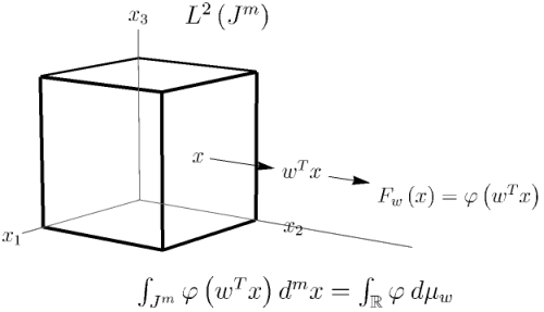
Given $F\in L^{2}\left(J^{m}\right)$ , how do we get representations of $F$ in terms of coordinate functions $J^{m}\ni x\rightarrow w\cdot x\in\mathbb{R}$ ? Here, $w\cdot x=w^{T}x=w_{1}x_{1}+\cdots+w_{m}x_{m}$ .

If $L\in\mathscr{B}$ , a Borel set in $\mathbb{R}$ , then the respective measures $\mu_{w}$ and $\mu_{X}$ from Figures 1.2 & 1.3 are as follows (distributions of random variables):

(1.10)		$\displaystyle\mu_{w}\left(L\right)$	$\displaystyle=\lambda_{m}\left(\left\{x\in J^{m}\mid X_{w}\left(x\right):=w^{T}x\in L\right\}\right),$
(1.11)		$\displaystyle\mu_{X}\left(L\right)$	$\displaystyle=\mathbb{P}\left(\left\{w\in\Omega\mid X\left(w\right)\in L\right\}\right).$

Equivalently, $\mu_{w}=\lambda_{m}\circ X_{w}^{-1}$ , and $\mu_{X}=\mathbb{P}\circ X^{-1}$ ; see also (1.1) & (1.2).

Let $\mathscr{C}:=C_{b}\left(\mathbb{R},\mathbb{R}\right)$ or $C_{b}\left(\mathbb{R},\mathbb{C}\right)$ . For $\varphi\in\mathscr{C}$ , we consider $x\longrightarrow\varphi\left(w^{T}x\right)$ as a function on $J^{m}$ . See Figures 1.2–1.3. And we define the following subspace

(1.12)

\mathscr{H}\left(w\right)=\overline{\left\{\varphi\left(w^{T}x\right)\mathrel{;}\varphi\in\mathscr{C}\right\}}^{L^{2}\left(J^{m}\right)}.

(The overbar means closure, and the superscript refers to the norm.)

Question.

What are minimal subsets $W$ of vectors $w\in\mathbb{R}^{m}\backslash\left(0\right)$ such that the closed span of $\left\{\mathscr{H}\left(w\right)\right\}_{w\in W}$ is equal to $L^{2}\left(J^{m}\right)$ ?

For additional details regarding probability spaces, random variables and distributions, see e.g., [1, 2, 3, 4]. Also see [5, 6, 7, 8] for approximation and Kolmogorov’s superposition theorem.

Remark 1.5.

Our present results are partially motivated by the following question: “How do neural nets (NN) learn?” For example, consider a single (hidden) layer neural net. With a specified starting point given as an arbitrary $w$ (could be set to zero); how will it then be updated through “backward propagation”, or “backprop”, as each training example passes through the system? Note that the process aims for the output to then be able to approximate uniformly any continuous function, i.e., (in the language of learning machines) the system learns a hypothesis. One thing that makes this successful for neural network (NN) is that backprop is fast enough to be able to train very large networks.

However, if $w$ is fixed (none zero), and we modify $\varphi$ as in (1.12), then there are several related questions:

(i)

How to choose the initial $\varphi$ ?

In standard NN-models, $w$ is fixed from the outset as activation function. A popular choice in recent literature is the rectified linear unit (ReLU); see e.g., [9]. Other options include sigmoid, ArcTan, etc.
(ii)

As training examples pass through the system, how is $\varphi$ updated? One would expect a variant of backprop.
(iii)

Is this version of backprop, if exists, fast enough to handle large networks?

In view of (ii), getting the optimal $\varphi$ is harder than training $w$ in standard NNs. In a standard NN (assuming single layer), $\varphi$ is fixed, and $w$ is updated recursively. Note that $w$ lives in a finite dimensional space.

If $w$ is fixed instead (see (1.12)), training $\varphi$ means one seeks the optimal solution in the set of all continuous functions, or differentiable functions, satisfying certain conditions (see Section 2 below). The parameter $\varphi$ , now a function, must be modified slightly at each iteration. The ambient space for $\varphi$ is infinite-dimensional.

Example 1.6.

In the special case, when $\varphi$ is fixed, we have a standard NN-model which serves to “train” $w$ . See Figure 1.4 below. Our present setup is much more subtle, and it is hard to compare this to the case when $w$ is fixed, and $\varphi$ varies. Our present results serve to motivate a number of algorithmic approaches to the “hard” case.

In Figure 1.4, we illustrate the structure of a standard $L$ -layer neural net for multiclass classification. (For example, in classical handwritten digit recognition, the number of classes is 10. See Figure 1.5.) The parameters are specified as follows:

$\bullet$

$x\in M_{m,n}$ , $n$ training examples, each of dimension $m$ ;
$\bullet$

$y\in M_{k,n}$ , $k$ classes, where $y\left(\cdot,j\right)$ is the standard basis in $\mathbb{R}^{k}$ .
$\bullet$

$w_{j}\in M_{s_{j},s_{j-1}}$ ; $s_{j}=$ number of units in layer $j$ , $s_{0}=m$ .
$\bullet$

$b_{j}\in\mathbb{R}^{s_{j}}$ , “bias”.
$\bullet$

$g_{j}:M_{s_{j},n}\rightarrow M_{s_{j},n}$ , $g_{j}\left(z\right)=\left(g_{j}\left(z_{s,t}\right)\right)$ , for $z=\left(z_{st}\right)\in M_{s_{j},n}$ .

During the training process, the system iterates to approximate the optimal parameters:

$\bullet$

Forward propagation;
$\bullet$

Calculation of cost;
$\bullet$

Backward propagation to obtain $dw$ , $db$ ;
$\bullet$

Update parameters, $w=w-\beta dw$ , $b=b-\beta db$ , where $\beta>0$ denotes the learning rate.

$x\longrightarrow g_{1}\left(w_{1}\left(\cdot\right)+b_{1}\right)\longrightarrow g_{2}\left(w_{2}\left(\cdot\right)+b_{2}\right)\longrightarrow\cdots\longrightarrow g_{L}\left(w_{L}\left(\cdot\right)+b_{L}\right)$

Figure 1.4. basic structure of a standard

L

-layer neural net

Figure 1.5. Example: handwritten digit recognition.

2. Theorems by Cybenko and Kolmogorov

Our present investigations are motivated in part by the following Universal Approximation Theorem by Cybenko:

Theorem 2.1 (Cybenko [10, 11]).

Let $\varphi:\mathbb{R}\rightarrow\mathbb{R}$ be given, satisfying the following two conditions:

(i)

$\varphi$ is continuous, and
(ii)
the following two limits exist:
1. (a)
  
  $\lim_{t\rightarrow-\infty}\varphi\left(t\right)=0$ , and
2. (b)
  
  $\lim_{t\rightarrow+\infty}\varphi\left(t\right)=1$ .

Then the span of the double-indexed functions

(2.1)

\left\{\varphi\left(w^{T}x+\lambda\right)\right\}_{w\in\mathbb{R}^{m}\backslash\left(0\right),\,\lambda\in\mathbb{R}}

is uniformly dense in $C\left(J^{m}\right)$ .

Proof sketch.

The required reasoning is three fold. Specifically, the proof establishes the following three assertions:

(1)

The family of functions in (2.1) is dense in $C\left(J^{m}\right)$ $\Longleftrightarrow$ The integral of the function system (2.1) being zero for Borel measures $\mu$ on $\mathbb{R}$ of finite total variation, only when $\mu$ is zero.
(2)

Subcases: The integral with respect to $\mu$ is zero iff $\mu$ vanishes on all the half-planes, $\Pi_{w,s}$ , $\Pi_{w,s}^{+}$ and $\Pi_{w,s}^{-}$ ; see details below.
(3)

The half-planes generate the $\sigma$ -algebra on $J^{m}$ .

Since most of the ideas going into the proof may be found in the papers [10, 11], we shall be brief: We provide the following sketch for the benefit of the reader.

Let $\varphi$ be as specified, and let $\mu$ be a Borel measure on $\mathbb{R}$ of finite total variation. For $\lambda,s,t\in\mathbb{R}$ , and $w\in\mathbb{R}^{m}\backslash\left(0\right)$ , consider the following family of functions on $\mathbb{R}^{m}$ :

(2.2)

\varphi\left(\lambda\left(w^{T}x+s\right)+t\right),\quad x\in J^{m};

and set

	$\displaystyle\Pi_{w,s}$	$\displaystyle=\left\{x\in\mathbb{R}^{m}\mathrel{;}w^{T}x+s=0\right\},$
	$\displaystyle H_{w,s}^{+}$	$\displaystyle=\left\{x\in\mathbb{R}^{m}\mathrel{;}w^{T}x+s>0\right\},$

and

H_{w,s}^{-}=\left\{x\in\mathbb{R}^{m}\mathrel{;}w^{T}x+s<0\right\}.

Then

		$\displaystyle\lim_{\lambda\rightarrow+\infty}\int_{J^{m}}\varphi\left(\lambda\left(w^{T}x+s\right)+t\right)d\mu\left(x\right)$
	$\displaystyle=$	$\displaystyle\mu\left(H_{w,s}^{+}\right)+\varphi\left(t\right)\mu\left(\Pi_{w,s}\right);$

and

		$\displaystyle\lim_{\lambda\rightarrow-\infty}\int_{J^{m}}\varphi\left(\lambda\left(w^{T}x+s\right)+t\right)d\mu\left(x\right)$
	$\displaystyle=$	$\displaystyle\mu\left(H_{w,s}^{-}\right)+\varphi\left(t\right)\mu\left(\Pi_{w,s}\right).$

∎

For additional details regarding the approximation problems, see e.g., [12, 13, 14, 15, 16, 17].

A second motivation for our present considerations is Kolmogorov’s superposition theorem. The latter in turn is Kolmogorov’s reply to Hilbert’s 13th Problem.

Theorem 2.2 (Kolmogorov, see [8]).

Let $f:\left[0,1\right]^{n}\rightarrow\mathbb{R}$ be an arbitrary multivariable continuous function. Then it has the representation

f\left(x_{1},\dots,x_{n}\right)=\sum_{q=0}^{2n}\Phi_{q}\left(\sum_{p=1}^{n}\psi_{q,p}\left(x_{p}\right)\right),

with continuous one-dimensional outer and inner functions $\Phi_{q}$ and $\psi_{q,p}$ . All these functions $\Phi_{q}$ and $\psi_{q,p}$ are defined on the real line. The inner functions $\psi_{q,p}$ are independent of the function $f$ .

Hilbert originally posed his 13th problem for algebraic functions (Hilbert 1927, “…Existenz von algebraischen Funktionen…”, i.e., “…existence of algebraic functions…”.) Hilbert asked for a process whereby a function of several variables may possibly be constructed using only functions of two variables. Hilbert’s conjecture, that it is not always possible to find such a solution, was disproven in 1957.

However, there also was a later version of the problem where Hilbert asked instead whether there are solution in the class of continuous functions. It is the second version of Hilbert’s 13th problem that concerns us here, by way of motivation. More specifically, a generalization of the second (“continuous”) variant of Hilbert’s problem is the question: Can every continuous function of three variables be expressed as a composition of finitely many continuous functions of two variables? The affirmative answer to this general question was given in 1957 by Vladimir Arnold. Earlier Kolmogorov had shown that any function of several variables can be constructed with a finite number of three-variable functions. Arnold then expanded on this work to show that only two-variable functions were in fact required, thus answering Hilbert’s question in the context of continuous functions. In our present consideration, we shall consider versions of the question for functions on the hyper cube $J^{m}$ , where $m$ is finite, but “large.” For the multivariable functions, we shall consider both the continuous case, as well as the variant for the problem in the Hilbert space $L^{2}\left(J^{m}\right)$ .

2.1. An infinite-dimensional analogue of Cybenko’s theorem

Let $\dot{\mathbb{R}}$ denote the one-point compactification of $\mathbb{R}$ , and consider the infinite product space

(2.3)

\Omega:=\dot{\mathbb{R}}^{\mathbb{N}}=\dot{\mathbb{R}}\times\dot{\mathbb{R}}\times\dot{\mathbb{R}}\times\cdots.

On $\Omega$ , we shall consider the topology generated by the cylinder sets; so that $\Omega$ is compact, by the Tychonov-theorem.

The $\sigma$ -algebra generated by the cylinder-sets will be denoted $\mathscr{F}$ ; and we shall be considering probability spaces $\left(\Omega,\mathscr{F},\mathbb{P}\right)$ .

A system $\mathscr{W}$ of random variables $X:\Omega\rightarrow\mathbb{R}$ is said to be separating iff (Def) the following subsets of $\Omega$ generate $\mathscr{F}$ :

(2.4)

\begin{split}\left\{X\left(\cdot\right)>s\right\}&=X^{-1}\left((s,\infty]\right),\;\text{and}\\ \left\{X\left(\cdot\right)=s\right\}&=X^{-1}\left(\left\{s\right\}\right),\end{split}

where $s\in\mathbb{R}$ , and $X\in\mathscr{W}$ are arbitrary. More precisely, we require that, if a signed measure $\mu$ on $\left(\Omega,\mathscr{F}\right)$ of finite total variation vanishes on the sets in (2.4), then $\mu$ must be zero.

Theorem 2.3.

Let $\left(\Omega,\mathscr{F},\mathbb{P}\right)$ be as above; let $\mathscr{W}$ be a separating system of continuous random variables; and let $\varphi:\mathbb{R}\rightarrow\mathbb{R}$ be a fixed function satisfying conditions (i) & (ii) in Theorem 2.1. Then the span of the double-indexed system of functions (on $\Omega$ ),

(2.5)

\left\{\varphi\left(X\left(\cdot\right)+\lambda\right)\right\}_{X\in\mathscr{W},\,\lambda\in\mathbb{R}}

is uniformly dense in $C\left(\Omega\right)$ ; i.e., dense w.r.t. the $\left\|\cdot\right\|_{\infty}$ -norm on $C\left(\Omega\right)$ .

Proof.

As the present arguments are close to those outlined in the proof of Theorem 2.1 above, we shall only sketch the details.

First consider the following system of functions on $\Omega$

(2.6)

\varphi\left(\lambda\left(X\left(\cdot\right)+s\right)+t\right)

where $\varphi$ is as stated, i.e., satisfying conditions (i) & (ii) in Theorem 2.1; and where $X\in\mathscr{W}$ , and $\lambda,s,t\in\mathbb{R}$ .

Let $\mu$ be a signed measure on $\left(\Omega,\mathscr{F}\right)$ of finite total variation. We now show that if

\int_{\Omega}\varphi\left(\lambda\left(X\left(\cdot\right)+s\right)+t\right)d\mu=0

for all $X\in\mathscr{W}$ , and $\lambda,s,t\in\mathbb{R}$ , then $\mu=0$ . But

		$\displaystyle\lim_{\lambda\rightarrow+\infty}\int_{\Omega}\varphi\left(\lambda\left(X\left(\cdot\right)+s\right)+t\right)d\mu$
		$\displaystyle=$		$\displaystyle\mu\left(\left\{X\left(\cdot\right)+s>0\right\}\right)+\varphi\left(t\right)\mu\left(\left\{X\left(\cdot\right)+s=0\right\}\right),$

and the desired conclusion now follows precisely as in Cybenko’s reasoning. Recall that the family $\mathscr{W}=\left\{X\left(\cdot\right)\right\}$ of random variables was assumed to be separating for $\left(\Omega,\mathscr{F}\right)$ . ∎

Corollary 2.4.

Consider the probability space $\left(\Omega,\mathscr{F},\mathbb{P}\right)$ in (2.3) where $\mathscr{F}$ is the product-cylinder $\sigma$ -algebra of subsets in $\Omega$ . For $\omega=\left(x_{j}\right)_{j\in\mathbb{N}}\in\Omega$ , set

(2.7)

X_{j}\left(\omega\right)=x_{j}\in\mathbb{R}.

Then the algebra $\mathscr{A}$ generated by

(2.8)

\left\{\varphi\circ X_{j}\mathrel{;}j\in\mathbb{N},\>\varphi\in\mathscr{C}\right\}

is uniformly dense in $C\left(\Omega\right)$ .

Proof.

By Stone-Weierstrass, we only need to verify that the algebra $\mathscr{A}$ from (2.8) separates points in $\Omega$ . But, if $\omega\neq\omega^{\prime}$ in $\Omega$ , then there is an index $j$ such that $X_{j}\left(\omega\right)\neq X_{j}\left(\omega^{\prime}\right)$ . Then just pick a $\varphi\in\mathscr{C}$ s.t. $\varphi\left(X_{j}\left(\omega\right)\right)\neq\varphi\left(X_{j}\left(\omega^{\prime}\right)\right)$ . ∎

3. Projective space of equivalence classes

Notation.

We shall work with projective space $P\left(\mathbb{R}^{m}\right)$ , i.e., equivalence classes in $\mathbb{R}^{m}\backslash\left(0\right)$ , where $w\sim w^{\prime}\Longleftrightarrow\exists t\in\mathbb{R}\backslash\left(0\right)\text{ s.t. $w^{\prime}=tw$}$ . Set

(3.1)

\mathscr{H}\left(w\right):=closure\left\{\varphi\left(w^{T}x\right),\;\varphi\in\mathscr{C}:=C\left(\mathbb{R},\mathbb{C}\right)\right\}.

The closure in (3.1) is w.r.t the $\left\|\cdot\right\|_{\infty}$ -norm of $C\left(J^{m}\right)$ , or the $L^{2}\left(J^{m}\right)$ -norm on $L^{2}\left(J^{m}\right)$ ; both cases are of interest. Note, if $w\sim w^{\prime}$ , then $\mathscr{H}\left(w\right)=\mathscr{H}\left(w^{\prime}\right)$ .

We discuss measures $\mu$ of finite total variation on $J^{m}$ such that

(3.2)

\displaystyle\int_{J^{m}}\varphi\left(w^{T}x\right)d\mu\left(x\right)

\displaystyle=0,\quad\forall\varphi\in\mathscr{C}.

And in the $L^{2}\left(J^{m}\right)$ case, we consider $F\in L^{2}\left(J^{m}\right)$ such that

(3.3)

\int_{J^{m}}\varphi\left(w^{T}x\right)F\left(x\right)d^{m}x=0,\quad\forall\varphi\in\mathscr{C}.

Lemma 3.1.

Equation (3.3) is included in the condition on $\mu$ from (3.2).

Proof.

Take $\mu$ of the form

(3.4)

d\mu=F\left(x\right)d^{m}x.

Viewed as signed measure, we have $d\mu\ll d^{m}x$ , where $d^{m}x$ is standard Lebesgue measure on $J^{m}$ . ∎

Remark 3.2.

For all $F\in L^{2}\left(J^{m}\right)\subset L^{1}\left(J^{m}\right)$ , the total variation measure $\left|\mu\right|$ from (3.4) is $d\left|\mu\right|\left(x\right)=\left|F\left(x\right)\right|d^{m}x$ . Recall that, for all Borel measurable sets $B$ in $J^{m}$ , we have

(3.5)

\left|\mu\right|\left(B\right):=\sup\left\{\sum\nolimits_{i}\left|\mu\left(A_{i}\right)\right|\right\}

where $\left\{A_{i}\right\}$ runs over all partitions of $B$ , i.e., $B=\cup_{i}A_{i}$ , $A_{i}\cap A_{j}=\emptyset$ if $i\neq j$ .

More generally, we shall make use of the following: Let $\Omega$ be a compact space, then $C\left(\Omega\right)$ with norm $\left\|\cdot\right\|_{\infty}$ , as a Banach space, has for its dual $\mathscr{M}:=\left\{\text{all signed measures on $\Omega$ of finite variation}\right\}$ with $\left\|\mu\right\|_{*}=\left|\mu\right|\left(\Omega\right)$ (see (3.5)) as the dual norm via $\mu\left(F\right)=\int_{\Omega}F\,d\mu$ , $F\in C\left(\Omega\right)$ .

Definition 3.3.

Set

\mathscr{A}\left(W\right)=\left\{\varphi\left(w^{T}x\right)\mathrel{;}w\in W,\;\varphi\in C\left(\mathbb{R},\mathbb{C}\right)\right\}.

Observations.

If $W=\left(\pi\mathbb{Z}\right)^{m}=$ Fourier lattice, then $\mathscr{A}\left(W\right)$ is dense in $C\left(J^{m}\right)$ , and therefore also dense in $L^{2}\left(J^{m}\right)$ . In this case, we will then only need $\varphi\left(t\right):=e^{it}$ , $t\in\mathbb{R}$ ; or, in the real case, $\varphi_{c}\left(t\right)=\cos t$ , $\varphi_{s}\left(t\right)=\sin t$ .

Proof.

Follows from Stone-Weierstrass; or Fejér-Cesàro. If $\varphi\left(t\right)=e^{it}$ , then $\varphi\left(w\cdot x\right)=e^{iw\cdot x}$ , $w\in\left(\pi\mathbb{Z}\right)^{m}$ , is the usual Fourier basis. Cesàro summation yields $\left\|\cdot\right\|_{\infty}$ approximation in $C\left(J^{m}\right)$ . ∎

4. Multivariable Fourier expansions

The setting of our approximation problem discussed below is related to that of Cybenko’s Theorem 2.1, but different. Nonetheless, the framework of Cybenko’s paper serves as motivation for our present considerations. Below we briefly outline differences, beginning with the starting point.

Recall, in Cybenko’s setting, there is only one given, and fixed, continuous function $\varphi$ on the real line $\mathbb{R}$ , but subject to the conditions listed in (ii). So, given $\varphi$ as in (ii), we allow variation of all $m$ -vectors, and all translation by real numbers. The conclusion of Theorem 2.1 yields approximation of all continuous functions on $J^{m}$ .

In the setting below, the starting point is different: We fix a set $W$ of $m$ -vectors, and, as in Cybenko, we ask for best approximation of functions on $J^{m}$ , in $C\left(J^{m}\right)$ or $L^{2}$ . But, in the present setting, we shall allow variation over all bounded continuous functions $\varphi$ on $\mathbb{R}$ . Also the given set $W$ will now in fact be considered a subset of projective space $P\left(\mathbb{R}^{m}\right)$ . One of our results states that $W$ -approximation of classes of functions on $J^{m}$ will not be possible when $W$ is finite. Hence we shall also consider countably infinite subsets $W$ of $P\left(\mathbb{R}^{m}\right)$ , and we shall address orthogonal decompositions as well, and an associated harmonic analysis. Our approach will be constructive.

Fourier coefficients of functions $F$ in $\mathscr{H}\left(w\right)$ , where $w\in\mathbb{Z}^{m}\backslash\left(0\right)$ is fixed:

Let $\mathscr{H}\left(w\right)$ be as in (3.1). Set

F\left(x\right):=\varphi\left(w^{T}x\right)=\sum_{k\in\mathbb{Z}}a_{k}e^{i\pi kw\cdot x},

where $\varphi\left(s\right)=\sum_{k\in\mathbb{Z}}a_{k}e^{i\pi ks}$ , $s\in\mathbb{R}$ , is the 1D Fourier expansion of $\varphi$ ; so $F$ is supported, in the Fourier domain, by the set $\mathbb{Z}w=\left\{kw\mathrel{;}k\in\mathbb{Z}\right\}$ . We shall use the usual notation:

	$\displaystyle kw\cdot x$	$\displaystyle=kw_{1}x_{1}+kw_{2}x_{2}+\cdots+kw_{m}x_{m},\quad k\in\mathbb{Z},$
	$\displaystyle w$	$\displaystyle=\left(w_{1},\cdots,w_{m}\right)\in\mathbb{Z}^{m}\backslash\left(0\right),\;\text{and}$
	$\displaystyle x$	$\displaystyle=\left(x_{1},\cdots,x_{m}\right)\in\mathbb{R}^{m}.$

Fix $w$ . Let $P_{W}$ be the projection from $L^{2}\left(J^{m}\right)$ onto

(4.1)

\mathscr{H}_{W}:=\overline{span}^{L^{2}\left(J^{m}\right)}\left\{\varphi\left(w^{T}x\right)\mathrel{;}\varphi\in C\left(\mathbb{R},\mathbb{R}\right),\;w\in W\right\}.

Thus, $P_{W}\left(f\right)$ is the unique $L^{2}\left(J^{m}\right)$ -minimizer:

(4.2)

\left\|f-P_{W}f\right\|_{L^{2}}=\inf\left\{\left\|f-g\right\|_{L^{2}}\mathrel{;}g\in\mathscr{H}_{W}\right\}.

However, it is not always easy to find a formula for $P_{W}f$ .

Notation.

In the case of $L^{2}\left(J^{m}\right)$ , we can simply form the closure of the subspace $\left\{\varphi\left(w^{T}x\right)\right\}_{w\in W,\,\varphi\in C}$ , i.e., closure in the $L^{2}\left(J^{m}\right)$ -norm. We write

(4.3)

W_{2}^{\perp}=\mathscr{H}_{W}^{\perp}:=L^{2}\left(J^{m}\right)\ominus\mathscr{H}_{W}=P_{W}^{\perp}L^{2}\left(J^{m}\right).

And so the functions $F\in W_{2}^{\perp}$ are simply the functions $F$ s.t. $P_{W}\left(F\right)=0$ , where $\mathscr{H}_{W}$ is as in (4.1), and $P_{W}=P_{\mathscr{H}_{W}}$ is the orthogonal projection in $L^{2}\left(J^{m}\right)$ onto $\mathscr{H}_{W}$ ; see (4.2).

Fix a subset $W\subset\mathbb{R}^{m}\backslash\left(0\right)$ . For a function $F$ on $J^{m}$ or on $\mathbb{R}^{m}$ , consider the two actions; translation and scaling:

	$\displaystyle\left(T_{y}F\right)\left(x\right)$	$\displaystyle=F\left(x+y\right),\quad$		$\displaystyle y\in\mathbb{R}^{m},$
	$\displaystyle\left(S_{a}F\right)\left(x\right)$	$\displaystyle=F\left(ax\right),$		$\displaystyle a\in\mathbb{R}.$

(If $F$ is a function on $J^{m}$ , translation is modulo by $2\mathbb{Z}$ .)

The invariance properties are for both the approximation problems in $C\left(J^{m}\right)$ and in $L^{2}\left(J^{m}\right)$ . Below we recall properties of the operators of translation $T_{y}$ and of scaling $S_{a}$ .

Lemma 4.1.

Both the subspace $\mathscr{H}_{W}$ , and the orthogonal complement $W_{2}^{\perp}$ , are invariant under the two actions $\left\{T_{y}\right\}$ and $\left\{S_{a}\right\}$ .

Definition 4.2.

Let $\mathscr{M}$ denote the Borel measures $\mu$ on $J^{m}$ of finite total variation.

In the case of $C\left(J^{m}\right)$ , we study $\mu\in\mathscr{M}$ s.t.

(4.4)

\int_{J^{m}}\varphi\left(w^{T}x\right)d\mu\left(x\right)=0,\quad\forall\varphi\in\mathscr{C},\;\forall w\in W,

where $\mathscr{C}=C_{b}\left(\mathbb{R},\mathbb{R}\right)$ , or $C_{b}\left(\mathbb{R},\mathbb{C}\right)$ .

In the case of $L^{2}\left(J^{m}\right)$ , we consider $F$ satisfying

(4.5)

\int_{J^{m}}F\left(x\right)\varphi\left(w^{T}x\right)d^{m}x=0,\quad\forall\varphi\in\mathscr{C},\;\forall w\in W,

i.e., $F\perp\left\{\varphi\left(w^{T}x\right)\right\}_{w\in W}$ in $L^{2}\left(J^{m}\right)$ .

Lemma 4.3.

$\mu\in\mathscr{M}$ satisfies (4.4) iff

(4.6)

\widehat{\mu}\left(tw\right)=0,\quad\forall t\in\mathbb{R},\;\forall w\in W.

The solution (in $L^{2}\left(J^{m}\right)$ ) to (4.5) is

(4.7)

\widehat{F}\left(tw\right)=0,\quad\forall t\in\mathbb{R},\;\forall w\in W.

Here, $\widehat{F}$ is the following Fourier transform:

(4.8)

\widehat{F}\left(\xi\right):=\int_{J^{m}}e^{i\xi\cdot x}F\left(x\right)d^{m}x,\quad\forall\xi\in\mathbb{R}^{m}.

Definition 4.4.

For $\mu,\nu\in\mathscr{M}$ (see Definition 4.2), we denote by $\mu\ast\nu$ the convolution given by

\int\varphi\,d\left(\mu\ast\nu\right):=\int_{J^{m}}\int_{J^{m}}\varphi\left(x+y\right)d\mu\left(x\right)d\nu\left(y\right),\quad\varphi\in\mathscr{C}.

Note that $\left(\mu\ast\nu\right)^{\wedge}=\widehat{\mu}\,\widehat{\nu}$ , pointwise product. The algebra $\left\{\widehat{\mu}\mathrel{;}\mu\in\mathscr{M}\right\}$ is called the Fourier algebra.

Lemma 4.5.

Fix a subset $W\subset\mathbb{R}^{m}\backslash\left(0\right)$ . Then

(4.9)

W_{\mathscr{M}}^{\perp}=\left\{\mu\in\mathscr{M}\mathrel{;}\widehat{\mu}\left(tw\right)=0,\;\forall t\in\mathbb{R},\>\forall w\in W\right\}

is an ideal in the convolution algebra. Equivalently, the Fourier transforms $\left\{\widehat{\mu}\mathrel{;}\mu\in W_{\mathscr{M}}^{\perp}\right\}$ is an ideal in the Fourier algebra.

Proof.

Immediate from the definitions. ∎

Remark 4.6 (Analytic continuation of $\widehat{\mu}$ and $\widehat{F}$ ).

Note that both $\widehat{\mu}\left(\cdot\right)$ and $\widehat{F}\left(\cdot\right)$ are entire analytic, and so extend to $\mathbb{C}^{m}$ ; $\xi\in\mathbb{R}^{m}\longrightarrow\mathbb{C}^{m}$ .

The notation of the function $\widehat{F}\left(\xi\right)$ in (4.8), $\xi\in\mathbb{R}^{m}$ , is reasonably well understood. The extension from $\mathbb{R}^{m}$ to $\mathbb{C}^{m}$ is as follows: Set

\widehat{F}\left(\zeta\right)=\underset{\widehat{G}\left(\zeta\right)}{\underbrace{\int_{J^{m}}e^{i\left(x_{1}\zeta_{1}+\cdots+x_{m}\zeta_{m}\right)}F\left(x\right)d^{m}x}}

where $\widehat{G}\left(\zeta\right)$ is an entire analytic function of exponential type, i.e.,

|\widehat{G}\left(\zeta\right)|\leq const\>e^{2\sum_{1}^{m}\left|\Im\zeta_{j}\right|}.

This is known as a Paley-Wiener class, and is reasonably well understood; see e.g., books by Hörmander [18, 19].

5. A Radon Transform

Recall that the Radon transform (see e.g., [20]) is an integral transform taking a function $f$ defined on the plane to a function $Rf$ defined on the (two-dimensional) space of lines in the plane, whose value at a particular line is equal to the line integral of the function over that line. Below we need a higher dimensional variant (see Lemma 5.1) of this idea, and we shall refer to it also as a Radon transform.

Lemma 5.1 (Radon transform).

With the measure in $L^{2}\left(J^{m}\right)$ , we obtain explicit formulas: Fix $W\subset\mathbb{R}^{m}\backslash\left(0\right)$ , and for $w\in W$ , set

(5.1)

\Pi_{w}=\left\{y\in\mathbb{R}^{m}\mathrel{;}w^{T}y=0\right\},

i.e., the hyperplane (Figure 5.1); then

(5.2)		$\displaystyle F\in L^{2}\left(J^{m}\right)\ominus\mathscr{H}_{W}$
	$\displaystyle\Updownarrow$
(5.3)		$\displaystyle\int_{y\in\Pi_{w}}F\left(sw+y\right)d\sigma_{w}\left(y\right)=0,\;\forall w\in W,\>\forall s\in\mathbb{R},$

where $d\sigma_{w}=d\sigma_{w}^{m-1}$ is the standard Lebesgue measure on $\Pi_{w}\simeq\mathbb{R}^{m-1}$ . Note that (5.3) is a Radon-transform. (See, e.g., [21, 22].)

Figure 5.1. The hyperplane

\Pi_{w}

Proof.

Fix $W\subset\mathbb{R}^{m}\backslash\left(0\right)$ . Assume without loss of generality that $\left\|w\right\|_{2}=1$ . For $x\in\mathbb{R}^{m}$ , set $y=x-\left(w^{T}x\right)w$ , then $y\in\Pi_{w}$ i.e., $w^{T}y=0$ by a direct calculation.

Introduce a coordinate system $\mathbb{R}\times\Pi_{w}\longleftrightarrow\mathbb{R}^{m}$ ,

\left(s,y\right)\longmapsto x=sw+y\in\mathbb{R}^{m}

with $s\in\mathbb{R}$ , $y\in\Pi_{w}$ ( $w$ is fixed and normalized); then

\int\varphi\left(w^{T}x\right)F\left(x\right)d^{m}x=\int\varphi\left(s\right)\left(\int_{y\in\Pi_{w}}F\left(sw+y\right)d\sigma_{w}\left(y\right)\right)ds.

It follows that

F\in W_{2}^{\perp}\Longleftrightarrow\int_{y\in\Pi_{w}}F\left(sw+y\right)d\sigma_{w}\left(y\right)=0,\quad\forall w\in W,\>\forall s\in\mathbb{R}.

∎

Corollary 5.2.

For $w\in\mathbb{R}^{m}\backslash\left(0\right)$ , let $\Pi_{w}$ and $d\sigma_{w}$ be as above. Define the following operator (Radon transform) $R_{w}:L^{2}\left(J^{m}\right)\longrightarrow L_{loc}^{2}\left(\mathbb{R}\right)$ ,

(5.4)

\left(R_{w}\left(F\right)\right)\left(t\right):=\int_{y\in\Pi_{w}}F\left(tw+y\right)d\sigma_{w}\left(y\right),\quad t\in\mathbb{R},

then

F\in L^{2}\left(J^{m}\right)\ominus\left\{\varphi\left(w^{T}x\right)\right\}_{\varphi\in\mathscr{C},\,w\in W}\Longleftrightarrow R_{w}\left(F\right)\equiv 0.

Proof.

We have

\int_{\mathbb{R}}\varphi\left(t\right)\left(R_{w}F\right)\left(t\right)dt=\left(Jac\right)\int_{J^{m}}\varphi\left(w^{T}x\right)F\left(x\right)d^{m}x,

where “ $Jac$ ” denotes the corresponding Jacobian. ∎

Here is another corollary of the duality approach:

Corollary 5.3.

If $W\subset\mathbb{R}^{m}\backslash\left(0\right)$ is given and finite, then

F\in L^{2}\left(J^{m}\right)\ominus\left\{\varphi\left(w^{T}x\right)\right\}_{\varphi\in\mathscr{C},\,w\in W}\Longleftrightarrow R_{w}F=0,\;\forall w\in W

is infinite dimensional.

It follows in particular that the space of solutions $\mu$ to

\int_{J^{m}}\varphi\left(w^{T}x\right)d\mu\left(x\right)=0,\quad\forall\varphi\in\mathscr{C},\>\forall w\in W,

is infinite-dimensional (i.e., $\mu\in W_{\mathscr{M}}^{\perp}$ , see (4.9)).

Below is a property that holds for functions $\varphi\left(w^{T}x\right)$ and not for other functions $F$ in $C\left(J^{m}\right)$ or in $L^{2}\left(J^{m}\right)$ :

Lemma 5.4.

Fix $w$ and $\varphi$ , and set $F\left(x\right)=\varphi\left(w^{T}x\right)$ , then $F$ is constant on every hyperplane

\Pi_{w,t}:=\left\{x\in\mathbb{R}^{m}\mathrel{;}w^{T}x=t\right\}.

Proof.

If $F\left(x\right)=\varphi\left(w^{T}x\right)$ , $x\in\Pi_{w,t}$ , then $F\left(x\right)=\varphi\left(t\right)$ . But we will need to also compute $\varphi\left(w^{T}x\right)$ when $w\neq w_{0}$ in $\mathbb{R}^{m}$ and $x\in\Pi_{w_{0},t_{0}}$ . The function is not constant on $\Pi_{w_{0},t}$ but it depends on only one angle.

In details, let $w\neq w_{0}$ be as above, and suppose $x\in\Pi_{w_{0},t_{0}}$ . Write

w=\alpha w_{0}+w^{T}

where $w^{T}\cdot w_{0}=0$ . Then $\varphi\left(w\cdot x\right)=\varphi\left(t_{0}\alpha+w^{\perp}\cdot x\right)$ . ∎

Corollary 5.5.

Let $W\subset\mathbb{R}^{m}\backslash\left(0\right)$ be a finite subset, then

\left\{\varphi\left(w^{T}x\right)\right\}_{\varphi\in\mathscr{C},\,w\in W}

is not dense in $L^{2}\left(J^{m}\right)$ .

Proof.

For every $w\in W$ , let $\left\{R_{w}\right\}_{w\in W}$ be the system of Radon transforms in $L^{2}\left(J^{m}\right)$ , see (5.4), i.e.,

R_{w}\left(F\right)\left(t\right)=\int_{y\in\Pi_{w}}F\left(tw+y\right)d\sigma_{w}^{\left(m-1\right)}\left(y\right),\quad t\in\mathbb{R}.

We consider function $G\in ker\left(R_{w}\right)$ , so $G\perp_{L^{2}\left(J^{m}\right)}\mathscr{H}_{W}$ . Suppose $W=\left\{w_{i}\right\}_{i=1}^{p}$ , then the functions

(5.5)

K:=G_{w_{1}}\ast G_{w_{2}}\ast\cdots\ast G_{w_{p}}\perp_{L^{2}\left(J^{m}\right)}\mathscr{H}_{W},

as $G_{w_{i}}\in ker\left(R_{w_{i}}\right)$ are chosen. Then $K$ is in $L^{2}\left(J^{m}\right)\ominus\mathscr{H}_{W}$ . The operation $\ast$ in (5.5) denotes convolution. ∎

6. Reproducing kernel and Shannon interpolation

Starting with $m=2$ , we shall display a complete list of points $w\in\mathbb{Z}^{2}\backslash\left(0\right)$ such that the corresponding subspaces $\mathscr{H}^{\prime}\left(w\right):=\mathscr{H}\left(w\right)\ominus\mathbb{C}\mathbbm{1}$ are mutually orthogonal. There is also the analogous question for $\mathbb{Z}^{m}$ , $m>2$ . The trick is to make a list of points $w$ in $\mathbb{Z}^{m}\backslash\left(0\right)$ such that the integer multiples $nw$ , $n\in\mathbb{Z}$ (i.e., integer lines), cover $\mathbb{Z}^{m}$ with no overlap other than in 0. The partitions of $\mathbb{Z}^{m}$ corresponds to equivalence classes in $\mathbb{Z}^{m}$ , hence non-overlap. We then make a system of orthogonal subspaces $\mathscr{H}^{\prime}\left(w\right)$ which is also total in $L^{2}\left(J^{m}\right)$ . This is made precise in Lemma 6.12; also see Examples 6.13–6.14.

The functions in (4.8) assume the multivariable Shannon interpolation, and $\{\widehat{F}\}_{F\in L^{2}\left(J^{m}\right)}$ is a reproducing kernel Hilbert space (RKHS) with the following Hilbert norm:

(6.1)

\|\widehat{F}\|_{RKHS}^{2}:=\left\|F\right\|_{L^{2}\left(J^{m}\right)}^{2}=\int_{J^{m}}\left|F\left(x\right)\right|^{2}d^{m}x.

See, e.g., [23, 24, 25, 26, 27].

The case $m>1$ , $L^{2}\left(J^{m}\right)$ , leads to a multivariable Shannon interpolation for the Fourier transform $\widehat{F}\left(\xi\right):=\int_{J^{m}}F\left(x\right)e^{ix\cdot\xi}d^{m}x$ , $\xi\in\mathbb{R}^{m}$ :

(6.2)

\displaystyle\widehat{F}\left(\xi\right)

\displaystyle=\sum_{\lambda\in\left(\mathbb{Z}/\pi\right)^{m}}\widehat{F}\left(\lambda\right)K_{m}\left(\xi-\lambda\right),\quad\forall\xi\in\mathbb{R}^{m},

where $\left(\mathbb{Z}/\pi\right)^{m}$ is the dual lattice, and $\widehat{F}\left(\lambda\right)$ are the Fourier coefficients.

Definition 6.1.

Fix $m$ , and $W\subset\mathbb{R}^{m}\backslash\left(0\right)$ a finite subset. Set

	$\displaystyle W_{\mathscr{M}}^{\perp}$	$\displaystyle:=\big\{\text{signed finite total variation measure $\mu$ on $J^{m}$ s.t.}$
		$\displaystyle\qquad\int\varphi\left(w^{T}x\right)d\mu\left(x\right)=0,\;\forall\varphi\in C_{b}\left(\mathbb{R},\mathbb{R}\right),\text{i.e.,}$
(6.3)			$\displaystyle\qquad\widehat{\mu}\left(tw\right)=0,\;\forall t\in\mathbb{R},\>\forall w\in W\big\}$

and

	$\displaystyle W_{2}^{\perp}$	$\displaystyle:=\big\{F\in L^{2}\left(J^{m}\right)\mathrel{;}\int_{J^{m}}\varphi\left(w^{T}x\right)F\left(x\right)d^{m}x=0,\;\forall\varphi,\;\text{i.e., }$
(6.4)			$\displaystyle\qquad\widehat{F}\left(tw\right)=0,\;\forall t\in\mathbb{R},\;\forall w\in W\big\}.$

The orthogonal complement “ $\perp$ ” in (6.4) refers to $L^{2}\left(J^{m}\right)$ . Note that $W_{2}^{\perp}\subset W_{\mathscr{M}}^{\perp}$ since, if $F\in L^{2}\left(J^{m}\right)$ , $d\mu\left(x\right)=F\left(x\right)d^{m}x$ is in $\mathscr{M}$ . (Also see (4.3), and Lemma 4.5.)

If we study approximations in $L^{2}\left(J^{m}\right)$ , then the question is: Fix $F\in L^{2}\left(J^{m}\right)$ s.t. $\left\langle F,\varphi\left(w^{T}x\right)\right\rangle_{L^{2}\left(J^{m}\right)}=0$ , $\forall w\in W$ , $\forall\varphi$ . We shall also consider signed measures $\mu$ s.t. $d\mu\left(x\right)=F\left(x\right)d^{m}x$ , then each condition for $\mu\in W_{\mathscr{M}}^{\perp}$ translates into $\widehat{F}\left(tw\right)=0$ , $\forall w\in W$ , $t\in\mathbb{R}$ . See Lemma 4.3.

More specifically, it follows from (6.2) that

(6.5)

\widehat{F}\left(tw\right)=\sum_{\lambda\in\left(\mathbb{Z}/\pi\right)^{m}}\widehat{F}\left(\lambda\right)K_{m}\left(tw-\lambda\right)

Equation (6.5) is entire analytic; and our condition takes the form:

	$\displaystyle\widehat{F}\left(tw\right)=0,\quad\forall t\in\mathbb{R}$
	$\displaystyle\Updownarrow$
	$\displaystyle\left(\frac{d}{dt}\right)^{k}\widehat{F}\left(tw\right)\Big\|_{t=0}=0,\quad\forall k\in\mathbb{N}_{0}$
	$\displaystyle\Updownarrow$
	$\displaystyle\sum_{\lambda\in\left(\mathbb{Z}/\pi\right)^{m}}\widehat{F}\left(\lambda\right)K_{m}^{\left(k\right)}\left(w-\lambda\right)=0,$
	$\displaystyle\forall w\in W,\>\forall k\in\mathbb{N}_{0}.$

Lemma 6.2.

Let $w,w^{\prime}\in\mathbb{Z}^{m}\backslash\left(0\right)$ , and assume $w\neq w^{\prime}$ ; then the following orthogonality relation holds:

(6.6)

\underset{\left\langle e_{w},e_{w^{\prime}}\right\rangle_{L^{2}\left(J^{m}\right)}}{\underbrace{\frac{1}{2^{m}}\int_{J^{m}}e^{i\pi w^{T}x}\overline{e^{i\pi w^{\prime T}x}}\,d^{m}x}}=\underset{\delta\left(w-w^{\prime}\right)}{\underbrace{\vphantom{\frac{1}{2^{m}}\int_{J^{m}}}\delta\left(w_{1}-w^{\prime}_{1}\right)\delta\left(w_{2}-w^{\prime}_{2}\right)\cdots\delta\left(w_{m}-w^{\prime}_{m}\right)}.}

Proof.

$L^{2}$ -inner products:

	$\displaystyle\text{LHS}_{\left(\ref{eq:F6}\right)}$	$\displaystyle=\frac{1}{2^{m}}\left(\int_{-1}^{1}e^{i\pi\left(w_{1}-w_{1}^{\prime}\right)x_{1}}dx_{1}\right)\left(\int_{-1}^{1}e^{i\pi\left(w_{2}-w_{2}^{\prime}\right)x_{2}}dx_{2}\right)\cdots$
		$\displaystyle\qquad\cdots\left(\int_{-1}^{1}e^{i\pi\left(w_{m}-w_{m}^{\prime}\right)x_{m}}dx_{m}\right)$
		$\displaystyle=\delta\left(w_{1}-w^{\prime}_{1}\right)\delta\left(w_{2}-w^{\prime}_{2}\right)\cdots\delta\left(w_{m}-w^{\prime}_{m}\right)$
		$\displaystyle=\delta\left(w-w^{\prime}\right)\quad\left(\text{in the abbreviated notation.}\right)$

∎

Lemma 6.3.

If $\varphi,\psi\in\mathscr{C}$ , we also get orthogonality when $w\neq w^{\prime}$ and inequivalent, then

(6.7)

\int_{J^{m}}\varphi\left(w^{T}x\right)\overline{\psi\left(w^{\prime T}x\right)}d^{m}x=0

unless $\varphi$ and $\psi$ contain constant components.

Proof.

Note the assumption is that $w$ and $w^{\prime}$ are inequivalent, so $kw\neq lw^{\prime}$ , $\forall k,l\in\mathbb{Z}\backslash\left(0\right)$ .

Use standard Fourier expansions for the two functions $\varphi$ and $\psi$ :

(6.8)

\varphi\left(s\right)=\sum_{k\in\mathbb{Z}}a_{k}e^{i\pi ks},\quad\psi\left(s\right)=\sum_{k\in\mathbb{Z}}b_{k}e^{i\pi ks},\quad s\in\mathbb{R}

with Fourier coefficients $\left(a_{k}\right)_{k\in\mathbb{Z}}$ and $\left(b_{k}\right)_{k\in\mathbb{Z}}$ . Now substitute (6.8) into (6.7),

(6.9)

\varphi\left(w^{T}x\right)=\sum_{k\in\mathbb{Z}}a_{k}e^{i\pi kw\cdot x},\;\text{and}\quad\psi\left(w^{T}x\right)=\sum_{l\in\mathbb{Z}}b_{l}e^{i\pi lw^{\prime}\cdot x},\quad x\in\mathbb{R}^{m},

then

\displaystyle\left\langle\varphi\left(w^{T}\cdot\right),\psi\left(w^{\prime T}\cdot\right)\right\rangle_{L^{2}\left(J^{m}\right)}

\displaystyle=\underset{k,\,l\in\mathbb{Z}}{\sum\sum}a_{k}\overline{b}_{l}\underset{=\delta\left(kw-lw^{\prime}\right)}{\underbrace{\int_{J^{m}}e^{i\pi\left(kw-lw^{\prime}\right)\cdot x}d^{m}x}},

which vanishes unless $k=l=0$ , and the latter correspond to the constant functions; see (6.9), i.e., $a_{k}=const\>\delta\left(k-0\right)$ , $b_{l}=const\>\delta\left(l-0\right)$ , $k,l\in\mathbb{Z}$ . ∎

In addition to the specific functions $F\in W_{2}^{\perp}$ we list above (covering some configurations), there are many more. Now we give a characterization which is based on orthogonality relations.

Example 6.4 (orthogonality, $m=2$ ).

If $m=2$ , then $F\left(x,y\right)=xy\in W_{2}^{\perp}$ where $W:=\left\{\left(\begin{smallmatrix}1\\ 0\end{smallmatrix}\right),\left(\begin{smallmatrix}0\\ 1\end{smallmatrix}\right)\right\}$ . To see this, one checks directly that

			$\displaystyle\int_{-1}^{1}\int_{-1}^{1}\left(f\left(x\right)+g\left(y\right)\right)xy\,\underset{d^{2}x}{\underbrace{dxdy}}$
		$\displaystyle=$	$\displaystyle\left\langle f\left(x\right)+g\left(y\right),F\right\rangle_{L^{2}\left(J^{2}\right)}$
		$\displaystyle=$	$\displaystyle\left(\int_{-1}^{1}xf\left(x\right)dx\right)\underset{=0}{\underbrace{\left(\int_{-1}^{1}ydy\right)}}+\underset{=0}{\underbrace{\left(\int_{-1}^{1}xdx\right)}}\left(\int_{-1}^{1}yf\left(y\right)dy\right)=0.$

Hence $F=xy$ is orthogonal to $\mathscr{H}_{W}$ . So $P_{W}\left(xy\right)=0$ , and

\inf_{g\in\mathscr{H}_{W}}\left\|xy-g\right\|_{L^{2}}^{2}=\left\|xy\right\|_{L^{2}}^{2}=\left(\frac{2}{3}\right)^{2}.

By the same argument, if $F\left(x,y\right)=\varphi\left(x\right)\psi\left(y\right)$ , assumed nonzero, where $\varphi$ and $\psi$ are odd functions, then $P_{W}F=0$ , and so

\inf_{g\in\mathscr{H}_{W}}\left\|F-g\right\|_{L^{2}}^{2}=\left\|F\right\|_{L^{2}}^{2}=\left(\int_{-1}^{1}\varphi^{2}dx\right)\left(\int_{-1}^{1}\psi^{2}dy\right)>0.

In particular, $W_{2}^{\perp}$ is infinite dimensional.

Example 6.5 ( $m=2$ ).

Let $W:=\left\{\left(\begin{smallmatrix}1\\ 0\end{smallmatrix}\right),\left(\begin{smallmatrix}0\\ 1\end{smallmatrix}\right)\right\}$ , and

\mathscr{A}_{W}=\left\{f\left(x\right)+g\left(y\right)\mathrel{;}f,g\in\mathscr{C}\right\}.

Then

(6.10)		$\displaystyle L^{2}\left(J^{2}\right)\ominus\mathscr{A}_{W}$	$\displaystyle=\Big\{F\in L^{2}\left(J^{2}\right)\;\text{s.t.}\int_{-1}^{1}F\left(x,\cdot\right)dx=0,$
		$\displaystyle\qquad\text{and }\int_{-1}^{1}F\left(\cdot,y\right)dy=0\Big\}.$

The functions $F$ may be written in terms of the Fourier expansions:

(6.11)

F=\underset{k,\,n\in\mathbb{Z}}{\sum\sum}c_{k,n}e^{i\pi\left(kx+ny\right)},\quad\left\|F\right\|_{L^{2}}^{2}=\underset{k,\,n\in\mathbb{Z}}{\sum\sum}\left|c_{k,n}\right|^{2}.

Then

	$\displaystyle f\in L^{2}\left(J^{2}\right)\ominus\mathscr{A}_{W}$
(6.12)		$\displaystyle\Updownarrow$
	$\displaystyle c_{0,n}=0,\;c_{k,0}=0,\quad\forall n,k\in\mathbb{Z}.$

Proof.

Compute the marginal Fourier coefficients in (6.11),

\int_{-1}^{1}F\left(x,y\right)dx=\sum_{n\in\mathbb{Z}}c_{0,n}e^{i\pi ny}=0,\quad\forall y

and

\int_{-1}^{1}F\left(x,y\right)dy=\sum_{k\in\mathbb{Z}}c_{k,0}e^{i\pi kx}=0,\quad\forall x,

and (6.12) follows. ∎

Hence we can rewrite all questions in terms of Fourier coefficients $c:=\left\{c_{k,n}\right\}_{k,n\in\mathbb{Z}}$ ,

F\longleftrightarrow c_{k,n}\underset{\text{Defn}}{\Longleftrightarrow}F\left(x,y\right)=\underset{k,n}{\sum\sum}c_{k,n}e^{i\pi\left(kx+ny\right)}.

And we have

	$\displaystyle P_{W}\left(c\right)$	$\displaystyle=span\left\{c_{k,0},c_{0,n}\right\}_{k,n\in\mathbb{Z}}$
		$\displaystyle=\begin{bmatrix}&&&\vdots\\ &&&c_{0,2}\\ &&&c_{0,1}\\ \cdots&c_{-2,0}&c_{-1,0}&c_{0,0}&c_{1,0}&c_{2,0}&\cdots\\ &&&c_{0,-1}\\ &&&c_{0,-2}\\ &&&\vdots\end{bmatrix}$

where $P_{W}$ is the projection onto $\mathscr{H}_{W}$ inside $L^{2}\left(J^{2}\right)$ .

Example 6.6.

Use of orthogonality of $\left\{e^{i\pi\left(kx+ny\right)}\right\}_{\left(k,n\right)\in\mathbb{Z}^{2}}$ . For example, if $F=Ae^{i\pi x}+Be^{i\pi\left(x+y\right)}$ then

dist\left(F,\mathscr{H}_{W}\right)=\inf_{g\in\mathscr{H}_{W}}\left\|F-g\right\|_{L^{2}\left(J^{2}\right)}=\left\|P_{W}^{\perp}F\right\|_{L^{2}\left(J^{2}\right)}=\left|B\right|;

since $P_{W}\left(F\right)=Ae^{i\pi x}$ , and $P_{W}^{\perp}\left(F\right)=Be^{i\pi\left(x+y\right)}$ .

The following computation works more generally for $\varphi\left(w^{T}x\right)$ , $\varphi\in C\left(\mathbb{R},\mathbb{C}\right)$ , $x=\left(x_{1},\cdots,x_{m}\right)$ , $w\in\mathbb{R}^{m}\backslash\left(0\right)$ fixed. But it is helpful to specialize to $m=2$ , $\left(x,y\right)\in\mathbb{R}^{2}$ , and $w=\left(\begin{smallmatrix}1\\ 0\end{smallmatrix}\right)=e_{1}$ ; we must then compute the Fourier coefficients of sum $e_{1}^{T}\left(x,y\right)=x$ .

In 2D, $F\left(x,y\right)=\varphi\left(x\right)$ , with Fourier coefficients indexed by $\mathbb{Z}^{2}$ :

	$\displaystyle c\left(n,k\right)$	$\displaystyle=\frac{1}{4}\iint_{J^{2}}\varphi\left(x\right)e^{-i\pi\left(nx+ky\right)}dxdy$
		$\displaystyle=\underset{\widehat{\varphi}\left(n\right)}{\underbrace{\frac{1}{2}\int_{-1}^{1}\varphi\left(x\right)e^{-i\pi nx}dx}}\>\underset{\delta\left(0-k\right)}{\underbrace{\frac{1}{2}\int_{-1}^{1}e^{-i\pi ky}dy}}$
		$\displaystyle=\widehat{\varphi}\left(n\right)\delta\left(0-k\right),\quad\forall\left(n,k\right)\in\mathbb{Z}^{2},$

where $\delta\left(0-k\right)=\begin{cases}1&\text{if $k=0$}\\ 0&\text{if $k\in\mathbb{Z}\backslash\left(0\right)$}\end{cases}$ .

Conclusion: $c\left(n,k\right)=\widehat{\varphi}\left(n\right)\delta\left(0-k\right)$ , $\forall\left(n,k\right)\in\mathbb{Z}^{2}$ , and

F\left(x,y\right)=\varphi\left(x\right)=\sum_{n\in\mathbb{Z}}\widehat{\varphi}\left(n\right)e^{i\pi nx}

which is the usual 1-dimensional Fourier expansion. This is a special case of a more general formula:

Consider $\mathbb{R}^{m}$ , $J^{m}$ , $W\subset\mathbb{R}^{m}\backslash\left(0\right)$ . Assume $w\in\mathbb{Z}^{m}$ , $w\in W$ fixed. Let $F\left(x\right)=\varphi\left(w^{T}x\right)$ , $x\in J^{m}$ , $\varphi:\mathbb{R}\longrightarrow\mathbb{C}$ (or $\mathbb{R}\longrightarrow\mathbb{R}$ ). Note $\varphi$ is a function on one coordinate. Without loss of generality, assume $\left\|w\right\|=1$ and let $P_{w}$ be the projection

	$\displaystyle P_{w}\left(x\right)$	$\displaystyle=\left(w^{T}x\right)w,\;\text{and}$
	$\displaystyle P_{w}\left(\mathbb{Z}^{d}\right)$	$\displaystyle=\left\{\left(w^{T}n\right)w\mathrel{;}n\in\mathbb{Z}^{d}\right\}$

then

F\left(x\right)=\sum_{\lambda\in P_{w}\left(\mathbb{Z}^{d}\right)}\widehat{\varphi}\left(\lambda\right)e^{i\pi\lambda P_{w}\left(x\right)}.

So if we select $w\in\mathbb{Z}^{m}\backslash\left(0\right)$ , then functions in $\mathscr{H}_{w}$ may give the Fourier expansion $F\left(x\right)=\varphi\left(w^{T}x\right)$ ,

F\left(x\right)=\sum_{k\in\mathbb{Z}}\widehat{\varphi}\left(k\right)e^{ikw^{T}x}

up to normalization. In the calculation of the 1D Fourier coefficients,

	$\displaystyle\widehat{\varphi}\left(k\right)$	$\displaystyle=\int_{-1}^{1}\varphi\left(x\right)e^{-i\pi ks}ds,\;\text{and}$
	$\displaystyle\varphi\left(s\right)$	$\displaystyle=\sum_{k\in\mathbb{Z}}\widehat{\varphi}\left(k\right)e^{i\pi ks},\quad s\in\mathbb{R},\>k\in\mathbb{Z}.$

In the general case, $w_{1},\cdots,w_{p}\in\mathbb{R}^{m}\backslash\left(0\right)$ , and may assume independent, and also a choice of $w_{k}\in\mathbb{Z}^{m}$ ; for $F\in\mathscr{H}_{w}$ ,

F\left(x\right)=\varphi_{1}\left(w_{1}^{T}x\right)+\varphi_{2}\left(w_{2}^{T}x\right)+\cdots+\varphi_{p}\left(w_{p}^{T}x\right)

$\varphi_{1},\varphi_{2},\cdots,\varphi_{p}\in\mathscr{C}:=C_{b}\left(\mathbb{R},\mathbb{C}\right)$ , or $C_{b}\left(\mathbb{R},\mathbb{R}\right)$ . After a renormalization,

	$\displaystyle F\left(x\right)$	$\displaystyle=\sum_{k\in\mathbb{Z}}\widehat{\varphi}_{1}\left(k\right)e^{ikw_{1}^{T}x}+\cdots+\sum_{k\in\mathbb{Z}}\widehat{\varphi}_{p}\left(k\right)e^{ikw_{p}^{T}x}$
		$\displaystyle=\sum_{\left(k_{1},\cdots,k_{p}\right)\in\mathbb{Z}^{m}}\sum_{j=1}^{p}\widehat{\varphi}_{j}\left(k_{j}\right)e^{i\pi k_{j}w_{j}^{T}x}.$

Lemma 6.7.

If $w,w^{\prime}\in P\left(\mathbb{R}^{m}\right)$ are distinct, equivalent class, then assume $w$ and $w^{\prime}$ both rational. The two subspaces $\mathscr{H}_{w}$ and $\mathscr{H}_{w^{\prime}}$ in $L^{2}\left(J^{m}\right)$ are orthogonal, i.e.,

(6.13)

\int_{J^{m}}F\left(x\right)\overline{F^{\prime}\left(x\right)}d^{m}x=0,\quad\forall F\in\mathscr{H}_{w},\;\forall F^{\prime}\in\mathscr{H}_{w^{\prime}}

unless the functions are constant.

Proof.

Select $w,w^{\prime}\in\mathbb{Z}^{m}\backslash\left(0\right)$ and compute the Fourier expansions of the two functions, $F\left(x\right)$ with coefficients in $\mathbb{Z}w$ , and $F^{\prime}\left(x\right)$ with coefficients in $\mathbb{Z}w^{\prime}$ . But since $w$ and $w^{\prime}$ are inequivalent,

(6.14)

\mathbb{Z}w\bigcap\mathbb{Z}w^{\prime}=0\;\text{in $\mathbb{Z}^{m}$}

and so the inner product in (6.13) $\equiv 0$ unless the two functions $F\in\mathscr{H}_{w}$ , and $F^{\prime}\in\mathscr{H}_{w^{\prime}}$ are constant. ∎

As $w$ varies over $\mathbb{Z}^{m}\backslash\left(0\right)$ , we get a system of orthogonal subspaces “nearly orthogonal” and if $w$ and $w^{\prime}$ are inequivalent,

\displaystyle\mathscr{H}\left(w\right)\cap\mathscr{H}\left(w^{\prime}\right)

\displaystyle=\text{constant multiples of the function $\mathbbm{1}$}

and $\mathscr{H}\left(w\right)\perp\mathscr{H}\left(w^{\prime}\right)$ except for the constants. Recall,

\mathscr{H}\left(w\right):=class^{L^{2}\left(J^{m}\right)}\left\{\varphi\left(w^{T}x\right)\mathrel{;}\varphi\in C\left(\mathbb{R},\mathbb{C}\right)\right\}.

An illustration of the subspaces in the case of $m=2$ , and $w\in\mathbb{Z}^{2}\backslash\left(0\right)$ . The property orthogonality for the subspace $\mathscr{H}^{\prime}\left(w\right):=\mathscr{H}\left(w\right)\ominus\mathbb{C}\mathbbm{1}$ , where $\mathbbm{1}$ is the constant function $\mathbbm{1}$ on $J^{m}$ . Hence

F\in\mathscr{H}^{\prime}\left(w\right)\Longleftrightarrow\int_{J^{m}}F\left(x\right)d^{m}x=0.

The argument above shows that

(6.15)

\mathscr{H}^{\prime}\left(w\right)\perp\mathscr{H}^{\prime}\left(w^{\prime}\right)

where $w$ and $w^{\prime}$ are inequivalent, so that

(6.16)

\int_{J^{m}}F\left(x\right)\overline{F^{\prime}\left(x\right)}d^{m}x=0,\quad\forall F\in\mathscr{H}^{\prime}\left(w\right),\>\forall F^{\prime}\in\mathscr{H}^{\prime}\left(w^{\prime}\right).

Below is a set of independent equivalent classes (and the subspaces are orthogonal), $k\in\mathbb{Z}\backslash\left(0\right)$ fixed.

$\left(0,k\right)$	$k\in\mathbb{Z}$	$class\left(0,1\right)$ : $\mathscr{H}\left(0,1\right)$
$\left(n,0\right)$	$n\in\mathbb{Z}$	$class\left(1,0\right)$ : $\mathscr{H}\left(1,0\right)$
$\left(n,n\right)$	$n\in\mathbb{Z}$	$class\left(1,1\right)$ : $\mathscr{H}\left(1,1\right)$
$\left(n,2n\right)$	$n\in\mathbb{Z}$	$class\left(1,2\right)$ : $\mathscr{H}\left(1,2\right)$
$\vdots$
$\left(n,kn\right)$	$n\in\mathbb{Z}$	$class\left(1,k\right)$ : $\mathscr{H}\left(1,k\right)$

Remark 6.8.

We may need the points in $\mathbb{Z}^{2}$ for an orthogonal in $L^{2}\left(J^{2}\right)$ , and we get orthogonal subspaces $\left\{\mathscr{H}\left(1,k\right)\right\}_{k\in\mathbb{Z}}$ , orthogonality modulo the constants. But if $w=\left(1,\sqrt{2}\right)$ for example, then the $\mathbb{Z}^{2}$ -representation is as follows

e^{i\pi\left(x+\sqrt{2}y\right)}=e^{i\pi x}\sum_{n\in\mathbb{Z}}\frac{\sin\pi\sqrt{2}}{\pi\left(\sqrt{2}-n\right)}e^{i\pi ny}\in\sum_{n\in\mathbb{Z}}^{\oplus}\mathscr{H}\left(1,n\right).

Moreover,

class\left(1,0\right)\cup class\left(0,1\right)\cup_{k\in\mathbb{Z}\backslash\left(0\right)}class\left(1,k\right)\cup class\left(\left(n_{1},n_{2}\right)\right)_{n_{1}\neq n_{2}}=\mathbb{Z}^{2};

see Example 6.4.

All the classes intersect in $\left(0,0\right)$ correspond to the index $c_{\left(0,0\right)}\mathbbm{1}$ , where $\mathbbm{1}=e^{i\pi\left(0x+0y\right)}$ in the 2D Fourier expansion:

\text{Fix $k$:$\quad$}\sum_{n\in\mathbb{Z}}a_{n}e^{i\pi n\left(x+ky\right)}\sim\mathscr{H}\left(\left(1,k\right)\right).

Question 6.9.

Display a complete list of points $w\in\mathbb{Z}^{2}\backslash\left(0\right)$ such that the corresponding subspaces $\mathscr{H}^{\prime}\left(w\right):=\mathscr{H}\left(w\right)\ominus\mathbb{C}\mathbbm{1}$ are mutually orthogonal.

Definition 6.10.

We say that a point in $class\left(w\right)$ is rational iff $\exists$ $\left(q_{1},\cdots,q_{m}\right)$ , $q_{i}\in\mathbb{Q}$ , such that $w\sim\left(q_{1},\cdots,q_{m}\right)$ . In this case, we may pick $\left(k_{1},\cdots,k_{m}\right)\in\mathbb{Z}^{m}$ such that $w\sim\left(k_{1},\cdots,k_{m}\right)$ .

A subset $W\subset\mathbb{R}^{m}\backslash\left(0\right)$ is said to be rational iff each class contains a rational generator. We get $\mathscr{H}_{W}=L^{2}\left(J^{m}\right)$ iff $W\subset P\left(\mathbb{R}^{m}\right)$ contains all the rational points.

Definition 6.11.

A subset $W\subset\mathbb{Z}^{m}\backslash\left(0\right)$ is said to be complete iff (Def.)

(6.17)		$\displaystyle\bigcup_{w\in W}\mathbb{Z}w$	$\displaystyle=\mathbb{Z}^{m};\;\text{and}$
(6.18)		$\displaystyle\mathbb{Z}w\bigcap\mathbb{Z}w^{\prime}$	$\displaystyle=0\;\text{when $w\neq w^{\prime}.$}$

Lemma 6.12.

If $W\subset\mathbb{Z}^{m}\backslash\left(0\right)$ is complete, then

(6.19)

\sum_{w\in W}^{\oplus}\mathscr{H}\left(w\right)=L^{2}\left(J^{m}\right),\;\text{with}

(6.20)

\mathscr{H}\left(w\right)\cap\mathscr{H}\left(w^{\prime}\right)=\mathbb{C}\mathbbm{1}\;\text{when $w\neq w^{\prime}$}.

And modulo constants, the subspaces are orthogonal. (In (6.20), $\mathbb{C}\mathbbm{1}$ denotes multiples of the constant function $\mathbbm{1}$ .)

Example 6.13 ( $m=2$ : Complete subsets in $\mathbb{Z}^{2}$ ).

Let

W=\left\{\left(1,0\right),\left(0,1\right),\left(n_{1},n_{2}\right)\right\},

where $g.c.d\left(n_{1},n_{2}\right)=1$ , and where g.c.d is short for the greatest common divisor (in $\mathbb{Z}_{+}$ ). See Figures 6.1–6.2.

Figure 6.1. Part of a complete subset in

\mathbb{Z}^{2}

Figure 6.2. A subset of vectors

w

in a set

W

having the completeness property from Example 6.13. Note that, for each discretized line, we are specifying a

w

yielding an irreducible direction; one for each of the equivalence classes in

\mathbb{Z}^{2}

, as illustrated in Figure 6.1 above. The idea is that, for a set

W

, we pick only one vector

w

for each of the discretized lines.

Example 6.14 ( $m>2$ : Complete subsets in $\mathbb{Z}^{m}$ ).

The union of the following subsets in $\mathbb{Z}^{m}\backslash\left(0\right)$ :

(i)

$\left(n_{1},n_{2},\cdots,n_{m}\right)\in\mathbb{Z}^{m}\backslash\left(0\right)$ , where $k$ out of the $m$ coordinates are $0$ , and $k=1,2,3,\cdots,m-1$ ; and g.c.d. for the non-zero coordinates = 1.
(ii)

$\left(n_{1},n_{2},\cdots,n_{m}\right)\in\mathbb{Z}^{m}\backslash\left(0\right)$ , where all $n_{j}\neq 0$ , $1\leq j\leq m$ , and $g.c.d\left\{n_{j}\right\}_{j=1}^{m}=1$ .

For additional details regarding reproducing kernel Hilbert spaces, see e.g., [28, 29, 30, 31].

7. Fourier representation

The purpose of this section is to make precise a certain Fourier/harmonic analysis representation for the UAT.

It suffices to take $\varphi\in C\left(\mathbb{R},\mathbb{C}\right)$ to be $2$ -periodic, i.e., $\varphi\left(s+2n\right)=\varphi\left(s\right)$ , $\forall s\in\mathbb{R}$ , $n\in\mathbb{Z}$ . We then have the usual Fourier expansion

	$\displaystyle\varphi\left(s\right)$	$\displaystyle=\sum_{n\in\mathbb{Z}}\widehat{\varphi}\left(n\right)e^{i\pi ns},$
	$\displaystyle\widehat{\varphi}\left(n\right)$	$\displaystyle=\frac{1}{2}\int_{-1}^{1}\varphi\left(s\right)e^{-i\pi ns}ds,$

and

\frac{1}{2}\int_{-1}^{1}\left|\varphi\left(s\right)\right|^{2}ds=\sum_{n\in\mathbb{Z}}\left|\widehat{\varphi}\left(n\right)\right|^{2}.

Now fix $w\in\mathbb{Z}^{m}\backslash\left(0\right)$ . Then

F\left(x\right):=\varphi\left(w^{T}x\right)=\varphi\left(w\cdot x\right)

has the representation

F\left(x\right)=\sum_{k\in\mathbb{Z}}\widehat{\varphi}\left(k\right)e^{i\pi kw^{T}x}=\sum_{k\in\mathbb{Z}}\widehat{\varphi}\left(k\right)e^{i\pi\left(kw\right)\cdot x};

and

\left\|F\right\|_{L^{2}\left(J^{m}\right)}^{2}=\frac{1}{2^{m}}\int_{J^{m}}\left|F\left(x\right)\right|^{2}d^{m}x=\sum_{k\in\mathbb{Z}}\left|\widehat{\varphi}\left(k\right)\right|^{2}.

Remark 7.1.

(i)

We consider annihilation measures $\mu\in W_{\mathscr{M}}^{\perp}$ , but these measures must necessarily be singular, albeit of finite total variation.
(ii)

Our reasoning here extends the argument given in Example 7.2 below. The setting in the example is specialized here in order to highlight the general idea.

(iii)

We begin with Parseval in one dimension as follows:

\int_{-\infty}^{\infty}\left|\psi\right|^{2}dx=\frac{1}{2\pi}\int_{-\infty}^{\infty}\left|\widehat{\psi}\left(\xi\right)\right|^{2}d\xi=2.

Fix $W\subset\mathbb{R}^{m}\backslash\left(0\right)$ . Recall $\mu\in W_{\mathscr{M}}^{\perp}\Longleftrightarrow$ $\mu_{w}=0$ $\forall w\in W$ $\Longleftrightarrow$ $\widehat{\mu}_{w}\equiv 0$ $\forall w\in W$ $\Longleftrightarrow$ $\widehat{\mu}\left(tw\right)=0$ $\forall t\in\mathbb{R}$ , $\forall w\in W$ . And one may apply this to $d\mu\left(x\right)=F\left(x\right)d^{m}x$ , $F\in L^{2}\left(J^{m}\right)$ .

Example 7.2 (Some wavelet functions, $m=2$ ).

Set $\psi=$ Haar wavelet function on $\mathbb{R}$ , up to normalization, so that

\widehat{\psi}\left(\xi\right)=\frac{\cos\left(\xi\right)-1}{\xi},\quad\xi\in\mathbb{R};

and $\widehat{\psi}\left(0\right)=0$ . Let

	$\displaystyle F_{1}\left(x_{1},x_{2}\right)$	$\displaystyle=f\left(x_{1}\right)\psi\left(x_{2}\right),$
	$\displaystyle F_{2}\left(x_{1},x_{2}\right)$	$\displaystyle=\psi\left(x_{1}\right)g\left(x_{2}\right),$

and $f,g$ are arbitrary. Then $F=F_{1}\ast F_{2}\in W^{\perp}$ , where $W=\left\{\left(\begin{smallmatrix}1\\ 0\end{smallmatrix}\right),\left(\begin{smallmatrix}0\\ 1\end{smallmatrix}\right)\right\}$ .

Similarly, for $m=3$ , set

	$\displaystyle F_{1}\left(x_{1},x_{2},x_{3}\right)$	$\displaystyle=f\left(x_{1},x_{2}\right)\psi\left(x_{3}\right),$
	$\displaystyle F_{2}\left(x_{1},x_{2},x_{3}\right)$	$\displaystyle=g\left(x_{1},x_{3}\right)\psi\left(x_{2}\right),$
	$\displaystyle F_{3}\left(x_{1},x_{2},x_{3}\right)$	$\displaystyle=h\left(x_{2},x_{3}\right)\psi\left(x_{1}\right),$

$f,g,h$ arbitrary. Then

F=F_{1}\ast F_{2}\ast F_{3}\in W^{\perp},

where $W=\left\{\left(\begin{smallmatrix}1\\ 0\\ 0\end{smallmatrix}\right),\left(\begin{smallmatrix}0\\ 1\\ 0\end{smallmatrix}\right),\left(\begin{smallmatrix}0\\ 0\\ 1\end{smallmatrix}\right)\right\}$ .

The first two terms in the Taylor expansion of $\widehat{\psi}\left(\xi\right)$ is

\widehat{\psi}\left(\xi\right)=-\frac{1}{2}\xi+\frac{1}{24}\xi^{3}-\cdots

In the remaining of the section, we discuss choices of sets $W$ of admissible directions to be used in our transform analysis. As well as some general properties for these sets.

Corollary 7.3.

$W^{\perp}$ is infinite-dimensional.

Now fix $w\in W$ , and do the $\psi$ construction in a concatenate system $\mathbb{R}w\times\Pi_{w}=\mathbb{R}^{m}$ , where $\Pi_{w}=\left\{x\in\mathbb{R}^{m}\mathrel{;}w^{T}x=0\right\}$ = the $w$ hyperplane.

For $z\in\Pi_{w}\backslash\left(0\right)$ , do a $\psi$ construction and extend to $\mathbb{R}^{m}$ , so

(7.1)

\widehat{\psi_{z}}\left(\xi\right)=\frac{\cos\left(z^{T}\xi\right)-1}{z^{T}\xi}=\frac{\cos\left(z\cdot\xi\right)-1}{z\cdot\xi},\quad\forall\xi\in\mathbb{R}^{m}.

But we should cut down $\psi_{z}$ to $J^{m}$ , so that integration is convergent.

Corollary 7.4.

Let $\psi_{z}$ be as above, and let $w$ be fixed; s.t. $w\in\Pi_{z}$ , $z\in\Pi_{w}$ . Then

(7.2)

\widehat{\psi}_{z}\left(tw\right)=0,\quad\forall t\in\mathbb{R},

and in particular, $\psi_{z}\in W_{2}^{\perp}$ .

Proof.

Observe that

(7.3)

\widehat{\psi}_{z}\left(tw\right)=\frac{\cos\left(tw^{T}z\right)-1}{tw^{T}z}=0

since $w^{T}z=0$ , see (7.1); so $\psi_{z}\in W_{2}^{\perp}\subset W_{\mathscr{M}}^{\perp}$ (but it depends on $w$ , fixed in $W$ .) If $W=\left\{w_{k}\right\}_{1}^{p}$ , and

(7.4)

\psi_{k}\in W_{2}^{\perp},

then

(7.5)

F=\ast_{k=1}^{p}\psi_{k}\in W_{2}^{\perp}

where $\ast$ denotes convolution. Note functions are restricted to $J^{m}$ . ∎

Here is a way to generate more functions $\psi_{k}$ as in (7.4)–(7.5): We can easily generalize to more functions $F\in W_{2}^{\perp}$ .

Fix $W=\left\{w_{k}\right\}_{1}^{p}$ . Let $\mu_{w_{1}}$ be a finite positive measure on $\Pi_{w_{1}}$ . Let $\psi_{z}$ be as in (7.1)–(7.2), $z\in\Pi_{w_{1}}$ , and set

(7.6)

\psi_{w_{1}}\left(\cdot\right)=\int_{\Pi_{w_{1}}}\psi_{z}\left(\cdot\right)d\mu_{w_{1}}\left(z\right)

as a function on $\mathbb{R}^{m}$ , and restrict to $J^{m}$ . Now do the construction in (7.6) also for $w_{2}$ , $w_{3}$ , $\cdots$ , $w_{p}$ , with choice of positive measures $\mu_{w_{k}}$ on $\Pi_{w_{k}}$ for $1\leq k\leq p$ ; and set

(7.7)

\psi=\ast_{k=1}^{p}\psi_{k},

so that $\widehat{\psi}=\prod_{k=1}^{p}\widehat{\psi}_{w_{k}}$ . We conclude that $\psi$ in (7.7) is in $W_{2}^{\perp}$ .

Example 7.5.

Illustration of key arguments in one and two dimensions.

For $m=2$ , $x=\left(x_{1},x_{2}\right)\in\mathbb{R}^{2}$ or $x\in J^{2}$ ; let $w=e_{2}$ and

\psi_{w_{2}}\left(x_{1},x_{2}\right)=\psi\left(x_{1}\right)

where $\psi$ is the 1D Haar wavelet. Then

	$\displaystyle\widehat{\psi_{w_{2}}}\left(\xi_{1},\xi_{2}\right)$	$\displaystyle=\int_{-1}^{1}\int_{-1}^{1}e^{i\left(x_{1}\xi_{1}+x_{2}\xi_{2}\right)}\psi\left(x_{1}\right)dx_{1}dx_{2}$
		$\displaystyle=\frac{\left(\cos\left(\xi_{1}\right)-1\right)}{\xi_{1}}\frac{\sin\left(\xi_{2}\right)}{\xi_{2}};$

recall $\text{sinc}\left(\xi\right)=\frac{\sin\xi}{\xi}$ . So we have

\widehat{\psi_{w_{1}}\ast\psi_{w_{2}}}\left(\xi_{1},\xi_{2}\right)=\frac{\cos\left(\xi_{2}\right)-1}{\xi_{2}}\text{sinc}\left(\xi_{1}\right)\frac{\cos\left(\xi_{1}\right)-1}{\xi_{1}}\text{sinc}\left(\xi_{2}\right)

and so $F=\psi_{w_{1}}\ast\psi_{w_{2}}\in W^{\perp}$ , where $W=\left\{\left(0,1\right),\left(1,0\right)\right\}$ , $\widehat{F}\left(tw_{1}\right)=0$ and $\widehat{F}\left(tw_{2}\right)=0$ , $\forall t\in\mathbb{R}$ .

$m$ -dimension ( $m>2$ ): Fix $w\in W$ , consider

\int_{\prod_{w}}\widehat{\psi_{z}}\left(tw\right)d\mu_{w}\left(z\right).

Set $F_{w}\left(x\right)=\int_{\Pi_{w}}\psi_{z}\left(x\right)d\mu_{w}\left(z\right)$ , then

\int_{J^{m}}\varphi\left(w^{T}x\right)F_{w}\left(x\right)d^{m}x

For additional details regarding Wiener theory and positive definite functions, see e.g., [32, 33].

Acknowledgement.

The present work was started during the NSF CBMS Conference, “Harmonic Analysis: Smooth and Non-Smooth”, by Jorgensen, held at the Iowa State University, June 4–8, 2018. We thank the NSF for funding, the organizers, especially Prof Eric Weber; and the CBMS participants. We had many fruitful discussions with Profs Daniel Alpay, and Sergii Bezuglyi, among others.

References

[1] T. Kaced, A. Romashchenko, and N. Vereshchagin, “A conditional information inequality and its combinatorial applications,” IEEE Trans. Inform. Theory, vol. 64, no. 5, pp. 3610–3615, 2018. [Online]. Available: https://doi.org/10.1109/TIT.2018.2806486
[2] J.-F. Mai, “Extreme-value copulas associated with the expected scaled maximum of independent random variables,” J. Multivariate Anal., vol. 166, pp. 50–61, 2018. [Online]. Available: https://doi.org/10.1016/j.jmva.2018.02.005
[3] M.-L. Tang, N.-S. Tang, P.-Y. Zhao, and H. Zhu, “Efficient robust estimation for linear models with missing response at random,” Scand. J. Stat., vol. 45, no. 2, pp. 366–381, 2018.
[4] A. H. Hamel and D. Kostner, “Cone distribution functions and quantiles for multivariate random variables,” J. Multivariate Anal., vol. 167, pp. 97–113, 2018. [Online]. Available: https://doi.org/10.1016/j.jmva.2018.04.004
[5] A. Khrennikov, “Reconstruction of quantum theory on the basis of the formula of total probability,” in Foundations of probability and physics—3, ser. AIP Conf. Proc. Amer. Inst. Phys., Melville, NY, 2005, vol. 750, pp. 187–218. [Online]. Available: https://doi.org/10.1063/1.1874572
[6] V. Brattka, “From Hilbert’s 13th problem to the theory of neural networks: constructive aspects of Kolmogorov’s superposition theorem,” in Kolmogorov’s heritage in mathematics. Springer, Berlin, 2007, pp. 253–280. [Online]. Available: https://doi.org/10.1007/978-3-540-36351-4_13
[7] P.-E. Leni, Y. D. Fougerolle, and F. Truchetet, “Kolmogorov superposition theorem for image compression,” IET Image Process., vol. 6, no. 8, pp. 1114–1123, 2012. [Online]. Available: https://doi.org/10.1049/iet-ipr.2011.0459
[8] J. Braun and M. Griebel, “On a constructive proof of Kolmogorov’s superposition theorem,” Constr. Approx., vol. 30, no. 3, pp. 653–675, 2009. [Online]. Available: https://doi.org/10.1007/s00365-009-9054-2
[9] V. Nair and G. E. Hinton, “Rectified linear units improve restricted boltzmann machines,” in Proceedings of the 27th International Conference on International Conference on Machine Learning, ser. ICML’10. USA: Omnipress, 2010, pp. 807–814. [Online]. Available: http://dl.acm.org/citation.cfm?id=3104322.3104425
[10] G. Cybenko, “Approximation by superpositions of a sigmoidal function,” Math. Control Signals Systems, vol. 2, no. 4, pp. 303–314, 1989. [Online]. Available: https://doi.org/10.1007/BF02551274
[11] ——, “Correction: “Approximation by superpositions of a sigmoidal function” [Math. Control Signals Systems 2 (1989), no. 4, 303–314; MR1015670 (90m:41033)],” Math. Control Signals Systems, vol. 5, no. 4, p. 455, 1992. [Online]. Available: https://doi.org/10.1007/BF02134016
[12] T. Kemmochi, “On the finite element approximation for non-stationary saddle-point problems,” Jpn. J. Ind. Appl. Math., vol. 35, no. 2, pp. 423–439, 2018. [Online]. Available: https://doi.org/10.1007/s13160-017-0293-5
[13] S. Harrap, M. Hussain, and S. Kristensen, “A problem in non-linear Diophantine approximation,” Nonlinearity, vol. 31, no. 5, pp. 1734–1756, 2018.
[14] A. Sheikholeslami and R. Ilati, “A sample average approximation approach to the berth allocation problem with uncertain tides,” Eng. Optim., vol. 50, no. 10, pp. 1772–1788, 2018. [Online]. Available: https://doi.org/10.1080/0305215X.2017.1411483
[15] G. Cybenko, “A general orthogonalization technique with applications to time series analysis and signal processing,” Math. Comp., vol. 40, no. 161, pp. 323–336, 1983. [Online]. Available: https://doi.org/10.2307/2007378
[16] ——, “Fast approximation of dominant harmonics,” SIAM J. Sci. Statist. Comput., vol. 5, no. 2, pp. 317–331, 1984. [Online]. Available: https://doi.org/10.1137/0905024
[17] G. Cybenko and V. Crespi, “Learning hidden Markov models using nonnegative matrix factorization,” IEEE Trans. Inform. Theory, vol. 57, no. 6, pp. 3963–3970, 2011. [Online]. Available: https://doi.org/10.1109/TIT.2011.2132490
[18] L. Hörmander, The analysis of linear partial differential operators. I, ser. Classics in Mathematics. Springer-Verlag, Berlin, 2003, distribution theory and Fourier analysis, Reprint of the second (1990) edition [Springer, Berlin; MR1065993 (91m:35001a)]. [Online]. Available: https://doi.org/10.1007/978-3-642-61497-2
[19] ——, The analysis of linear partial differential operators. II, ser. Classics in Mathematics. Springer-Verlag, Berlin, 2005, differential operators with constant coefficients, Reprint of the 1983 original. [Online]. Available: https://doi.org/10.1007/b138375
[20] G. Rigaud and A. Lakhal, “Approximate inverse and Sobolev estimates for the attenuated Radon transform,” Inverse Problems, vol. 31, no. 10, pp. 105 010, 21, 2015. [Online]. Available: https://doi.org/10.1088/0266-5611/31/10/105010
[21] S. Moon, “Properties of the fractional (exponential) Radon transform,” Integral Transforms Spec. Funct., vol. 28, no. 12, pp. 923–939, 2017. [Online]. Available: https://doi.org/10.1080/10652469.2017.1390666
[22] A. V. Baev, “Radon transform for solving an inverse scattering problem in a planar layered acoustic medium,” Comput. Math. Math. Phys., vol. 58, no. 4, pp. 537–547, 2018. [Online]. Available: https://doi.org/10.1134/S0965542518040061
[23] H. Dym, “On a class of monotone functions generated by ergodic sequences,” Amer. Math. Monthly, vol. 75, pp. 594–601, 1968. [Online]. Available: https://doi.org/10.2307/2313774
[24] D. Alpay and H. Dym, “Hilbert spaces of analytic functions, inverse scattering and operator models. I,” Integral Equations Operator Theory, vol. 7, no. 5, pp. 589–641, 1984. [Online]. Available: https://doi.org/10.1007/BF01195919
[25] D. Alpay, P. Dewilde, and H. Dym, “On the existence and construction of solutions to the partial lossless inverse scattering problem with applications to estimation theory,” IEEE Trans. Inform. Theory, vol. 35, no. 6, pp. 1184–1205, 1989. [Online]. Available: https://doi.org/10.1109/18.45275
[26] D. Alpay and H. Dym, “On a new class of structured reproducing kernel spaces,” J. Funct. Anal., vol. 111, no. 1, pp. 1–28, 1993. [Online]. Available: https://doi.org/10.1006/jfan.1993.1001
[27] P. L. Butzer, A. Fischer, and R. L. Stens, “Generalized sampling approximation of multivariate signals; general theory,” Atti Sem. Mat. Fis. Univ. Modena, vol. 41, no. 1, pp. 17–37, 1993.
[28] S. Lv, H. Lin, H. Lian, and J. Huang, “Oracle inequalities for sparse additive quantile regression in reproducing kernel Hilbert space,” Ann. Statist., vol. 46, no. 2, pp. 781–813, 2018. [Online]. Available: https://doi.org/10.1214/17-AOS1567
[29] L. Mei, Y. Jia, and Y. Lin, “Simplified reproducing kernel method for impulsive delay differential equations,” Appl. Math. Lett., vol. 83, pp. 123–129, 2018. [Online]. Available: https://doi.org/10.1016/j.aml.2018.03.024
[30] M. Mohammadi, F. Saberi Zafarghandi, E. Babolian, and S. Jvadi, “A local reproducing kernel method accompanied by some different edge improvement techniques: application to the Burgers’ equation,” Iran. J. Sci. Technol. Trans. A Sci., vol. 42, no. 2, pp. 857–871, 2018. [Online]. Available: https://doi.org/10.1007/s40995-016-0113-9
[31] N. Aronszajn, “Theory of reproducing kernels,” Trans. Amer. Math. Soc., vol. 68, pp. 337–404, 1950. [Online]. Available: https://doi.org/10.2307/1990404
[32] D. Gorbachev and S. Tikhonov, “Moduli of smoothness and growth properties of Fourier transforms: two-sided estimates,” J. Approx. Theory, vol. 164, no. 9, pp. 1283–1312, 2012. [Online]. Available: https://doi.org/10.1016/j.jat.2012.05.017
[33] D. V. Gorbachev and S. Y. Tikhonov, “Wiener’s problem for positive definite functions,” Math. Z., vol. 289, no. 3-4, pp. 859–874, 2018. [Online]. Available: https://doi.org/10.1007/s00209-017-1978-9

Superposition, reduction of multivariable problems, and approximation

Abstract.

Key words and phrases:

2000 Mathematics Subject Classification

1. Introduction

1.1. Infinite dimensions and a probabilistic framework

Definition 1.1.

The infinite dimensional case

Lemma 1.2.

Proof.

Proposition 1.3.

Proof.

Corollary 1.4.

Proof.

Question.

Question.

Remark 1.5.

Example 1.6.

2. Theorems by Cybenko and Kolmogorov

Theorem 2.1 (Cybenko [10, 11]).

Proof sketch.

Theorem 2.2 (Kolmogorov, see [8]).

2.1. An infinite-dimensional analogue of Cybenko’s theorem

Theorem 2.3.

Proof.

Corollary 2.4.

Proof.

3. Projective space of equivalence classes

Notation.

Lemma 3.1.

Proof.

Remark 3.2.

Definition 3.3.

Observations.

Proof.

4. Multivariable Fourier expansions

Fourier coefficients of functions FF in ℋ⁡(w)\mathscr{H}\left(w\right), where w∈ℤm\(0)w\in\mathbb{Z}^{m}\backslash\left(0\right) is fixed:

Notation.

Lemma 4.1.

Definition 4.2.

Lemma 4.3.

Definition 4.4.

Lemma 4.5.

Proof.

Remark 4.6 (Analytic continuation of μ^\widehat{\mu} and F^\widehat{F}).

5. A Radon Transform

Lemma 5.1 (Radon transform).

Proof.

Corollary 5.2.

Proof.

Corollary 5.3.

Lemma 5.4.

Proof.

Corollary 5.5.

Proof.

6. Reproducing kernel and Shannon interpolation

Definition 6.1.

Lemma 6.2.

Proof.

Lemma 6.3.

Proof.

Example 6.4 (orthogonality, m=2m=2).

Example 6.5 (m=2m=2).

Proof.

Example 6.6.

Lemma 6.7.

Proof.

Remark 6.8.

Question 6.9.

Definition 6.10.

Definition 6.11.

Lemma 6.12.

Example 6.13 (m=2m=2: Complete subsets in ℤ2\mathbb{Z}^{2}).

Example 6.14 (m>2m>2: Complete subsets in ℤm\mathbb{Z}^{m}).

7. Fourier representation

Remark 7.1.

Example 7.2 (Some wavelet functions, m=2m=2).

Corollary 7.3.

Corollary 7.4.

Proof.

Fourier coefficients of functions $F$ in $\mathscr{H}\left(w\right)$ , where $w\in\mathbb{Z}^{m}\backslash\left(0\right)$ is fixed:

Remark 4.6 (Analytic continuation of $\widehat{\mu}$ and $\widehat{F}$ ).

Example 6.4 (orthogonality, $m=2$ ).

Example 6.5 ( $m=2$ ).

Example 6.13 ( $m=2$ : Complete subsets in $\mathbb{Z}^{2}$ ).

Example 6.14 ( $m>2$ : Complete subsets in $\mathbb{Z}^{m}$ ).

Example 7.2 (Some wavelet functions, $m=2$ ).