Average Transmission Success Probability Bound for SWIPT Relay Networks

Since energy at the EH node is not automatically replenished as in a traditional node with fixed power supply, the performance of an EH network depends on the EH protocol and the usage scheme of the harvested energy. For simultaneous information and power transfer (SWIPT), two basic EH protocols, i) time-switching (TS) and ii) power-splitting (PS), are introduced for amplify-and-forward (AF) and decode-and-forward (DF) relay networks in [5, 6, 7]. An optimal hybrid EH protocol, which is a combination of PS and TS protocols is introduced in [8, 9] and it outperforms both TS and PS protocols. An improved receiver architecture for PS protocol is introduced in [10] and [11], which makes use of the level of the harvested energy as side information to assist the decoding of the source transmitted message. The common assumption of most of these work is that the total harvested energy is used for data transmission and thus a battery for long term energy storage is not required at the EH node. However, a long term energy storage enables a PS energy harvesting node to manage two basic resources i) PS ratio and ii) transmit energy. Thus, an efficient resource allocation scheme, which store excess amount of harvested energy for future use, can achieve a better performance compared to a network without a battery in the EH node. Due to the battery energy dependency on the resource allocation decisions made earlier, the analysis of the system performance needs more attention.

For EH relaying with a battery, several resource allocation methods are discussed in literature. An AF relaying network with TS energy harvesting is considered in [12], where data relaying is realized when sufficient energy is collected through EH. An AF relaying network with PS energy harvesting is considered in [13], where the remaining energy after data transmission is stored in the battery. The optimal resource allocation that maximizes the energy efficiency in a WSN with DF relaying is considered in [14]. A sum-throughput maximization problem is formulated for DF relay [15], where the relay node opportunistically switch between modes of total EH and PS based information processing. Resource allocation schemes for EH nodes which harvest energy from renewable sources such as wind or solar are investigated in [16, 17]. All these work assume full CSI at the decision node. The outage performance is analyzed in [18] for a sub-optimal resource allocation scheme based on incremental DF relay protocol.

In contrast to previous work [5, 6, 7, 8, 13, 12, 14, 15], this paper thus considers a dual hop DF relaying network with the PS energy harvesting protocol assuming that no CSI of forward channels is available at any node. The system performance is evaluated by the average success probability of the source to destination communication. To efficiently use the harvested energy, the relay is equipped with a battery, which consists of a finite capacity. In contrast to [18], we focus our attention to find the maximum average success probability over the set of resource allocation policies. The evaluation of maximum is important to assess the feasibility of the network for a practical set of system parameters. Due to the intractability of the problem, we develop a mathematical framework to find an upper bound for the maximum average success probability by formulating a discrete state Markov decision problem (MDP).

We consider a wireless relay network in which a source node (S) communicates with a destination node (D) via a single relay node (R). The relay operates in the DF mode. We assume that the direct link between S and D is not available due to a blockage. The communication takes place in half-duplex mode. Each node has a single antenna.

The network operates block by block, where each block has a duration $T$ and is indexed by $m\in\{1,2,\cdots\}$. The fading coefficients of S to R channel (S-R) and R to D channel (R-D) in the $m$th block are denoted by $\tilde{h}_{m}$ and $\tilde{g}_{m}$, respectively, which are independent. Since an unbounded flat-fading channel may be modeled by a finite number of channel states with an arbitrary low error [19, 13], both channel coefficients are drawn from finite sets. We assume that there is no feedback from D to R or from R to S. Thus, no CSI is available on the forward channel, i.e., S does not have any channel knowledge, R has knowledge on $\tilde{h}_{m}$, and D has knowledge on $\tilde{g}_{m}$. The source transmits with constant power $P_{s}$ and information rate $\tau$. The relay harvests energy from source transmitted information signal and uses that energy for information transmission to the destination. The PS protocol is used in R. The source transmits the message during the first half of the block. The relay uses $\sqrt{\lambda_{m}}$ portion of the received signal for the EH, and the remaining $\sqrt{1-\lambda_{m}}$ portion of the received signal is utilized for the information decoding. During the second half of the block, the relay transmits the decoded message to the destination using $u_{m}$ amount of energy.

The total harvested energy during the $m$th block by neglecting the noise energy, is $\eta P_{s}h_{m}\lambda_{m}\frac{T}{2}$ where $\eta\in(0,1)$ is the conversion efficiency [3]. This energy is directly transfered to the battery. Thus, the battery energy at $t=\left(m+\frac{1}{2}\right)T$ is

where $B<\infty$ is the battery capacity and $E_{m}$ is the residual battery energy at the beginning of the $m$th block.

For information transmission from R to D, the relay uses $u_{m}$ amount energy. The residual battery energy for the next block, is

If Shannon channel capacity is larger than the information rate $\tau$, the receiving node may decode the received signal with arbitrary small error probability. This is defined as a successful decoding. Thus, to achieve a successful decoding with a minimum received SNR $\gamma_{\tau}$, we have $\tau=\frac{1}{2}\mathrm{log}_{2}\left(1+\gamma_{\tau}\right)$ bits/s/Hz, in which the factor $\frac{1}{2}$ is due to each S-R and R-D links are used only half of the total time. This satisfies $\gamma_{\tau}=4^{\tau}-1$. Thus, for a successful decoding at the relay and the destination, we have $\gamma_{1}\left(h_{m},\lambda_{m}\right)\geqslant\gamma_{\tau}$ and $\gamma_{2}\left(g_{m},u_{m}\right)\geqslant\gamma_{\tau}$, respectively. The PS ratio $\lambda_{m}$ and relay transmit energy $u_{m}$ used, impact the SNRs $\gamma_{1}\left(h_{m},\lambda_{m}\right)$ and $\gamma_{2}\left(g_{m},u_{m}\right)$. Subsequently, they effect the probability of successful transmission from the source to the destination. In the next section, we discuss the calculation of the average success probability.

If the conditional distribution of the state $S_{m+1}$ given $S_{m}=s=\left(h,E\right)$ is known, the evaluation of expectation operation in (11) is straight forward. A simple way this can be achieved is by driving the energy level of the battery to zero by using the total amount of the battery energy for $u_{m}$. Thus, for any $S_{m}$, the residual battery energy $E_{m+1}=0$ and the $h_{m+1}$ is independent from $S_{m}$. With the aid of (6), a heuristic decision rule, which always drives the battery energy to zero can be given as

The stationary policy generated by the above decision rule is $\pi_{l}=d_{l}^{\infty}$. If $\pi_{l}$ is used, the states $S_{m}$ for all $m>1$ is known to be an element from the set $\left\{\left(0,h\right)|\ h\in\mathcal{H}\right\}$. Therefore, the average success probability for initial state $S_{1}=s$ can be written as

By taking the limit in the above equation and noting that $\widetilde{\text{P}}_{\pi_{l}}(s)$ is constant with respect to $s$, with the aid of (12) we have

This can be evaluated using (10) and (13) for each state $\left(0,h\right)$ with $h\in\mathcal{H}$ and taking the average using the probability mass function $f_{\mathcal{H}}$.

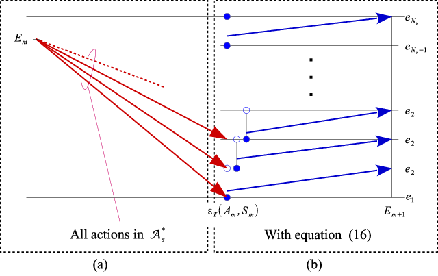
Although, the state transition of any policy can be modeled by a Markov chain, finding an upper bound using a MDP is involved due to the state space $\mathcal{S}$ is uncountably infinite. Therefore, instead of formulating a MDP for the original system model, we first appropriately modify the system to have a finite state space. We prove that the maximum of the average success probability of the finite state space system gives an upper bound for the maximum of the average success probability of the original system. To this end, we discretize the battery energy assuming that there exists a hypothetical energy source in the relay, which injects energy to the battery at the beginning of each block, such that battery energy occupy only predefined $N_{b}$ number of levels. For the current state $S_{m}$ and action $A_{m}$ the residual battery energy for the next block given in (4) is modified by the hypothetical energy source according to

Each $e_{i}=\frac{\left(i-1\right)B}{N_{b}-1}$ for all $i=1,\cdots,N_{b}$ denotes the finite battery levels in the battery. According to (15), the hypothetical energy source drives the battery energy to the nearest upper level defined by each $e_{i}$. This is shown in Fig. 1b. Thus, the state space has finite number of elements and we denote it by $\mathcal{S}^{\prime}=\left\{e_{1},\cdots,e_{N_{b}}\right\}\times\mathcal{H}$. We denote a general element of $\mathcal{S}^{\prime}$ by $s_{i}$, which are indexed in such a way, that states $\left(e_{j},h^{(1)}\right)$ to $\left(e_{j},h^{(N_{c})}\right)$ map with $s_{(jN_{c}-N_{c}+1)}$ to $s_{(jN_{c})}$, respectively. Due to the finite nature of the state space, one-step transition probability from the state $S_{m}$ to state $S_{m+1}$ for any decision rule $d$ can be given in a matrix form according to

If the current state is $s_{i}$ and the residual battery energy determined by the action is $e_{j}$, the $i$th row of the transition matrix $\Theta_{d}$ consists of the channel probability values $f_{\mathcal{H}}\left(h^{(1)}\right)$ to $f_{\mathcal{H}}\left(h^{(N_{c})}\right)$ from column $N_{c}\left(j-1\right)+1$ to column $N_{c}j$.

Since the state space is finite, for any decision rule $d$, we can define a reward vector $p_{d}$ in which, each element gives the reward for each state and action defined by the decision rule for the state, i.e. $p_{d}\left(s_{i}\right)=p\big(s_{i},d(s_{i})\big)$ for all $s_{i}\in\mathcal{S}^{\prime},\ d\in\mathcal{D}$. Using the transition matrix $\Theta_{d}$ and the reward vector $p_{d}$ we can write the average success probability of the modified system, in a vector form as [20]

The average success probability for the initial state $S_{1}=s_{i}$ is given by $\widetilde{\text{P}}^{\prime}_{\pi}\left(s_{i}\right)$, which is the $i$th element of the vector $\widetilde{\text{P}}^{\prime}_{\pi}$. Although the state space $\mathcal{S}^{\prime}$ is finite, the action space $\mathcal{A}_{s_{i}}$ for each $s_{i}\in\mathcal{S}^{\prime}$ is uncountably infinite for each $s_{i}$. However, the number of levels of residual battery energy is finite with the modification (15). Thus, we have groups of actions for which the resulting residual battery energy is the same. In fact, it is sufficient to consider a finite action space to find $\underset{\pi\in\Pi}{\text{max}}\ \widetilde{\text{P}}^{\prime}_{\pi}\left(s_{i}\right)$. This is proved in the next lemma and the proposition.

We prove that for any policy $\pi$ there exists a policy $\pi^{\prime}$ as given in the proposition such that $\Theta_{d_{m}}=\Theta_{d^{\prime}_{m}}$ and $p_{d^{\prime}_{m}}\geqslant p_{d_{m}}$ for all $m$, which essentially prove that $\widetilde{\text{P}}^{\prime}_{\pi^{\prime}}\geqslant\widetilde{\text{P}}^{\prime}_{\pi}$ with (17). Using lemma 1, there exists a decision rule $d^{\prime}_{m}$ in $\mathcal{A}^{\prime}_{s}$ that gives $\Theta_{d_{m}}=\Theta_{d^{\prime}_{m}}$. The dimension of $\mathcal{A}^{\prime}_{s}$ can be further reduced to have $p_{d^{\prime}_{m}}\geqslant p_{d_{m}}$. We consider cases $\mathcal{C}_{1}$ and $\mathcal{C}_{2}$ separately. (i) When $s\in\mathcal{C}_{1}$, as discussed $p_{d}\left(s\right)=0$ for all $d$. Therefore, we set $d^{\prime}\left(s\right)$ to take the corresponding element in $\mathcal{A}^{\prime}_{s,1}$ such that $\Theta_{d}\left(s\right)=\Theta_{d^{\prime}}\left(s\right)$. (ii) When $s\in\mathcal{C}_{2}$, $\lambda\leqslant\frac{hP_{s}-2\sigma^{2}\gamma_{\tau}}{hP_{s}-\sigma^{2}\gamma_{\tau}}$ is feasible for $\mathcal{A}_{s}$ and for $\mathcal{A}^{\prime}_{s}$. We consider two sub cases for $d\left(s\right)=\left(\lambda,u\right)$. (ii.a) When $\lambda\leqslant\frac{hP_{s}-2\sigma^{2}\gamma_{\tau}}{hP_{s}-\sigma^{2}\gamma_{\tau}}$. Let the residual battery energy resulted from $d\left(s\right)$ be $e_{i}$. We set the decision rule $d^{\prime}\left(s\right)=\left(\lambda^{\prime},E^{\prime}_{t}\right)\in\mathcal{A}^{\prime}_{s}$ such that $\lambda^{\prime}=\frac{hP_{s}-2\sigma^{2}\gamma_{\tau}}{hP_{s}-\sigma^{2}\gamma_{\tau}}$ and $\mathcal{E}_{T}\left(\lambda,u,s\right)=e_{i}$. It can be shown with (4) that this makes $E^{\prime}_{t}\geqslant u$, which results in $p_{d^{\prime}}\left(s\right)\geqslant p_{d}\left(s\right)$ in (10). It should be noted that $d^{\prime}\left(s\right)\in\mathcal{A}^{\prime}_{s,2}$. (ii.b) When $\lambda>\frac{hP_{s}-2\sigma^{2}\gamma_{\tau}}{hP_{s}-\sigma^{2}\gamma_{\tau}}$. In this situation $p_{d}\left(s\right)=0$. Therefore, we set $d^{\prime}\left(s\right)$ to take the corresponding element in $\mathcal{A}^{\prime}_{s,1}$. The new decision rules $d^{\prime}_{m}$ take only the elements in $\mathcal{A}^{\prime}_{s,1}\cup\mathcal{A}^{\prime}_{s,2}$ and we have $\Theta_{d_{m}}=\Theta_{d^{\prime}_{m}}$ and $p_{d^{\prime}_{m}}\geqslant p_{d_{m}}$ for all $m$, which proves $\widetilde{\text{P}}^{\prime}_{\pi^{\prime}}\geqslant\widetilde{\text{P}}^{\prime}_{\pi}$. This concludes the proof.

We first compare average success probability over $M$ blocks given in (11) for the two systems for a general $M$, where we denote it for the modified system by $\bar{p}^{\prime}_{\pi,M}$. We use the backward induction method to prove that $\underset{\pi}{\text{max}}\ \bar{p}^{\prime}_{\pi,M}\geqslant\underset{\pi}{\text{max}}\ \bar{p}_{\pi,M}$, which leads to the results in the proposition. Here, $\bar{p}^{\prime}_{\pi,M}$ is defined similar to $\bar{p}_{\pi,M}$ in (11)

For any given $S_{M}=\left(E_{M},h_{1,M}\right)$ the optimal decision rule that maximize $p\left(S_{M},d_{M}\left(S_{M}\right)\right)$ denoted by $d^{*}_{M}$ uses total energy in the relay battery. Therefore, if the state $S^{\prime}_{M}=\left(E^{\prime}_{M},h_{1,M}\right)$ is such that $E^{\prime}_{M}>E_{M}$ then $p\left(S^{\prime}_{M},d^{*}_{M}\left(S_{M}\right)\right)\geqslant p\left(S_{M},d^{*}_{M}\left(S_{M}\right)\right)$. For any given $S_{M-1}$ and action $A_{M-1}$ if the original system gives $S_{M}=\left(E_{M},h_{1,M}\right)$, the modified system gives $S^{\prime}_{M}=\left(E^{\prime}_{M},h_{1,M}\right)$ with $E^{\prime}_{M}\geqslant E_{M}$. Thus we have

Let the two states $S_{M-1}=\left(E_{M-1},h_{1,{M-1}}\right)$ and $S^{\prime}_{M-1}=\left(E^{\prime}_{M-1},h_{1,{M-1}}\right)$ be such that $E^{\prime}_{M-1}>E_{M-1}$ and let the optimal action for $S_{M-1}$ that maximize the sum

be $A^{*}_{M-1}$. Since $S^{\prime}_{M-1}$ has a lager battery energy, with the aid of (3) and (4) it can be seen that the action $A^{*}_{M-1}$ is feasible for $S^{\prime}_{M-1}$ and results in a larger $E_{M}$ compared taking the action $A^{*}_{M-1}$ in $S^{\prime}_{M-1}$. Thus we have

Thus the optimal action for $S^{\prime}_{M-1}$ denoted by $A^{**}_{M-1}$ should satisfy

References

- [1] J. G. Andrews, S. Buzzi, W. Choi, S. V. Hanly, A. Lozano, A. C. K. Soong, and J. C. Zhang, “What will 5G be?” IEEE J. Select. Areas Commun., vol. 32, no. 6, pp. 1065–1082, Jun. 2014.
- [2] S. Atapattu, N. Ross, Y. Jing, Y. He, and J. S. Evans, “Physical-layer security in full-duplex multi-hop multi-user wireless network with relay selection,” IEEE Trans. Wireless Commun., 2019, In press.
- [3] X. Zhou, R. Zhang, and C. K. Ho, “Wireless information and power transfer: Architecture design and rate-energy tradeoff,” IEEE Trans. Commun., vol. 61, no. 11, pp. 4754–4767, Nov. 2013.
- [4] C. X. Wang, F. Haider, X. Gao, X. H. You, Y. Yang, D. Yuan, H. M. Aggoune, H. Haas, S. Fletcher, and E. Hepsaydir, “Cellular architecture and key technologies for 5G wireless communication networks,” IEEE Commun. Mag., vol. 52, no. 2, pp. 122–130, Feb. 2014.
- [5] A. A. Nasir, X. Zhou, S. Durrani, and R. A. Kennedy, “Relaying protocols for wireless energy harvesting and information processing,” IEEE Trans. Wireless Commun., vol. 12, no. 7, pp. 3622–3636, Jul. 2013.
- [6] S. Atapattu, H. Jiang, J. Evans, and C. Tellambura, “Time-switching energy harvesting in relay networks,” in Proc. IEEE Int. Conf. Commun. (ICC), Jun. 2015, pp. 5416–5421.
- [7] S. Atapattu and J. Evans, “Optimal power-splitting ratio for wireless energy harvesting in relay networks,” in Proc. IEEE Vehicular Technology Conf. (VTC), Sep. 2015.
- [8] ——, “Optimal energy harvesting protocols for wireless relay networks,” IEEE Trans. Wireless Commun., vol. 15, no. 8, pp. 5789–5803, Aug. 2016.
- [9] B. Pilanawithana, S. Atapattu, and J. Evans, “Energy allocation and energy harvesting in wireless relay networks with hybrid protocol,” in Proc. IEEE Global Telecommun. Conf. (GLOBECOM), Dec 2017.
- [10] C. H. Chang, R. Y. Chang, and F. T. Chien, “Energy-assisted information detection for simultaneous wireless information and power transfer: Performance analysis and case studies,” IEEE Trans. Signal Inf. Process. Netw., vol. 2, no. 2, pp. 149–159, June 2016.
- [11] Y. Kim, D. K. Shin, and W. Choi, “Rate-energy region in wireless information and power transfer: New receiver architecture and practical modulation,” IEEE Transactions on Communications, vol. 66, no. 6, pp. 2751–2761, Jun. 2018.
- [12] I. Krikidis, S. Timotheou, and S. Sasaki, “Rf energy transfer for cooperative networks: Data relaying or energy harvesting?” IEEE Commun. Lett., vol. 16, no. 11, pp. 1772–1775, Nov. 2012.
- [13] Z. Zhou, M. Peng, Z. Zhao, W. Wang, and R. S. Blum, “Wireless-powered cooperative communications: Power-splitting relaying with energy accumulation,” IEEE J. Select. Areas Commun., vol. 34, no. 4, pp. 969–982, Apr. 2016.
- [14] T. Liu, X. Wang, and L. Zheng, “A cooperative swipt scheme for wirelessly powered sensor networks,” IEEE Trans. Commun., vol. 65, no. 6, pp. 2740–2752, June 2017.
- [15] G. Huang and W. Tu, “On opportunistic energy harvesting and information relaying in wireless-powered communication networks,” IEEE Access, vol. 6, pp. 55 220–55 233, 2018.
- [16] F. Yuan, Q. T. Zhang, S. Jin, and H. Zhu, “Optimal harvest-use-store strategy for energy harvesting wireless systems,” IEEE Trans. Wireless Commun., vol. 14, no. 2, pp. 698–710, Feb 2015.
- [17] M. Dong, W. Li, and F. Amirnavaei, “Online joint power control for two-hop wireless relay networks with energy harvesting,” IEEE Trans. Signal Processing, vol. 66, no. 2, pp. 463–478, Jan 2018.
- [18] G. Li and H. Jiang, “Performance analysis of wireless powered incremental relaying networks with an adaptive harvest-store-use strategy,” IEEE Access, vol. 6, pp. 48 531–48 542, 2018.
- [19] P. Sadeghi, R. A. Kennedy, P. B. Rapajic, and R. Shams, “Finite-state markov modeling of fading channels - a survey of principles and applications,” IEEE Signal Processing Mag., vol. 25, no. 5, pp. 57–80, Sep. 2008.
- [20] M. L. Puterman, Markov Decision Processes: Discrete Stochastic Dynamic Programming. Wiley-Interscience, 2005.