Complex-energy analysis of proton-proton fusion
Abstract
An analysis of the astrophysical factor of the proton-proton weak capture () is performed on a large energy range covering solar-core and early Universe temperatures. The measurement of being physically unachievable, its value relies on the theoretical calculation of the matrix element . Surprisingly, reaches a maximum near that has been unexplained until now. A model-independent parametrization of valid up to about is established on the basis of recent effective-range functions. It provides an insight into the relationship between the maximum of and the proton-proton resonance pole at from analytic continuation. In addition, this parametrization leads to an accurate evaluation of the derivatives of , and hence of , in the limit of zero energy.
I Introduction
The proton-proton fusion reaction (), also known as the proton-proton weak capture, is a fundamental process in nuclear astrophysics. It is the starting point of the proton-proton chain for stellar nucleosynthesis in hydrogen-burning stars. Its cross section is usually expressed in terms of the astrophysical factor at the two-proton center-of-mass energy . Unfortunately, this cross section is so small at typical astrophysical temperature (), that a reliable measurement cannot be achieved with enough statistics, even above the Coulomb barrier (about ). A theoretical prediction of is therefore required.
The first calculation of at zero energy was proposed by Bethe and Critchfield Bethe and Critchfield 1938. They also introduced the dimensionless weak capture matrix element at zero angular momentum from which they deduced . Thereafter, the accuracy of was improved by Salpeter Salpeter 1952 and Bahcall and his coworkers Bahcall and May 1969 using effective-range theory. In the 1990s, several authors calculated from the nucleon-nucleon wave functions computed in potential models Bahcall and Pinsonneault 1992; Kamionkowski and Bahcall 1994. More recently, systematic computations of were performed in pionless effective field theory from next-to-leading order (NLO) of the momentum expansion Kong and Ravndal 2001; Ando et al. 2008 up to N4LO Butler and Chen 2001. In parallel, efforts were made in chiral effective field theory to reduce the uncertainty on by adding two-body corrections to the Gamow-Teller operator adjusted with data for tritium -decay Carlson et al. 1991; Park et al. 2003; Schiavilla et al. 1998; Marcucci et al. 2013; *Marcucci2014a. As the uncertainty on has diminished since early works, the small contribution of its energy derivatives and has become important for nuclear astrophysics Adelberger et al. 2011; Marcucci et al. 2013; *Marcucci2014a; Chen et al. 2013; Acharya et al. 2016. In this regard, Adelberger et al. recommended a calculation of to be undertaken Adelberger et al. 2011.
The calculation of these derivatives raises the question of whether is analytic in the neighborhood of zero energy. Such an analysis is still missing in the literature. Yet, some peculiarities of the proton-proton scattering are known. In 1980, Kok highlighted the presence of a sub-threshold resonance pole at about in the channel Kok 1980. Up to a complex phase, this pole lies in an energy range corresponding to early Universe temperatures below the nucleosynthesis freeze-out point () Tanabashi et al. 2018. Therefore, the derivatives of are likely to be influenced by the relative closeness of this pole. In addition, it is known that the Coulomb interaction between two protons generates a sequence of poles at complex energy which accumulate to the zero-energy point Kok 1980; Gaspard and Sparenberg 2018. These poles may affect the polynomial extrapolation used in Refs. Schiavilla et al. 1998; Marcucci et al. 2013; *Marcucci2014a; Acharya et al. 2016 to determine , , and from the numerical computation of on an energy range that does not include . In this context, the issue is to understand the influence of all these structures on the astrophysical factor.
The purpose of this work is to obtain an efficient model-independent parametrization of , valid on a large energy range (), and able to impose constraints on its series expansion at . Our parametrization must also describe the resonance pole at and the Coulomb poles. To do so, we resort to a recently introduced effective-range function (ERF), namely the function Ramírez Suárez and Sparenberg 2017; Gaspard and Sparenberg 2018; Baye and Brainis 2000, which has only been considered useful for heavier systems until now Blokhintsev et al. 2017; *Blokhintsev2018a; *Blokhintsev2018b. This approach is motivated by the efficiency of the ERFs at describing the energy-dependent shape of the proton-proton wave function up to a few MeVs. It is aimed to reach a much better accuracy on the values of , , and than with the polynomial extrapolation performed in Refs. Schiavilla et al. 1998; Marcucci et al. 2013; *Marcucci2014a; Acharya et al. 2016. Finally, our results will be verified with the nucleon-nucleon wave functions computed in different local potential models, namely Av18 Wiringa et al. 1995, Reid93 Stoks et al. 1994, and NijmII Stoks et al. 1994. In particular, these potentials are intended to validate the model independence of our parametrization.
This paper is organized as follows. Section II presents the parametrization of the astrophysical factor, first from analytical approximations of the nucleon-nucleon wave functions in Subsec. II.2, and then in a model-independent way in Subsec. II.3. The analysis of at complex energies is discussed in Sec. III and supplemented by graphical illustrations. The numerical values of the logarithmic derivatives of are shown in Sec. IV. Section V is devoted to a conclusion. Detailed calculations of the Fermi phase-space integral and the Coulomb integrals are given in Appendices A and B, respectively.
II Proton-proton weak capture
II.1 Astrophysical factor
Let us start by defining the astrophysical factor studied in this paper. After integrating out the emitted leptons, the proton-proton weak capture cross section is known to be given to a good approximation by Salpeter 1952; Bahcall and May 1969; Baye 2013
| (1) |
where is the proton-proton wave number, and and are the radial -wave components of the deuteron and proton-proton wave functions respectively. The contribution from higher-order partial waves can be neglected in the low-energy approximation Acharya et al. 2019. The parameter is the weak axial/vector ratio, is the dimensionless weak coupling constant for neutrons, is the Fermi constant of muon decay, and is the first element of the CKM quark mixing matrix. All the fundamental constants are taken from Ref. Tanabashi et al. 2018. The quantity in Eq. (1) is known as the Fermi phase-space integral, which accounts for the electric repulsion of the emitted positron in a relativistic framework. It is discussed in more detail in Appendix A.
It turns out that the overlap integral between and in Eq. (1) vanishes in the zero energy limit (). This vanishing behavior originates from the cancellation of the proton-proton radial wave function at due to the Coulomb barrier. This behavior can be factored out of the overlap integral in defining the dimensionless orbital matrix element as Salpeter 1952; Bahcall and May 1969
| (2) |
where is the Coulomb normalization coefficient, is the Sommerfeld parameter, and is the proton-proton Bohr radius. The other constants are the deuteron binding wave number Bahcall and May 1969; Adelberger et al. 2011, the proton-neutron reduced mass , and the deuteron binding energy . In contrast to the overlap integral, has a finite limit at . With these notations, the cross section (1) becomes after some simplifications
| (3) |
This expression (3) suggests the most natural definition of the astrophysical factor, that is
| (4) |
This definition (4) of is assumed in this work. Strictly speaking, the definition (4) does not reduce to the original definition due to Salpeter Salpeter 1952
| (5) |
and nowadays considered as standard in stellar astrophysics. We point out that Eq. (4) is considered in Sec. II of Bahcall’s and May’s paper Bahcall and May 1969, even though they actually defined by Eq. (5).
Anyway, at sufficiently low energy, the definitions (4) and (5) coincide. We notice indeed that the approximation is valid within less than for
| (6) |
where is the nuclear Rydberg energy which is equal to in the proton-proton system. Since we consider energies much higher than the Rydberg energy in this work, definition (4) is preferred. Thus, we understand Eq. (5) as the low-energy approximation of Eq. (4).
Furthermore, it should be noted that definition (4) does not affect any of the values , , and presented in the main text compared to . Indeed, the relative error between the two definitions displays an essential singularity at which cancels all its derivatives in the limit . Therefore, the derivatives of at obtained in this work are necessarily equal to the derivatives of at .
Finally, using Eqs. (3) and (4), one finds the expression
| (7) |
The currently recommended value of is Adelberger et al. 2011.
II.2 Wave function-based parametrization
Most of the energy dependence in the overlap integral (2) comes from the proton-proton wave function . This function is normalized such that it tends to a sine wave of unit amplitude for . Its asymptotic behavior reads
| (8) |
where and are the standard Coulomb wave functions Olver et al. 2010, and is the proton-proton phase shift. Similarly, the asymptotic behavior of the deuteron wave function is
| (9) |
The normalization coefficient is found to be using three different potential models (Av18, Reid93, and NijmII) Wiringa et al. 1995; Stoks et al. 1994. It turns out that the asymptotic regime in Eqs. (8) and (9) is already reached for . Since the spatial extent of the deuteron is much larger than , it is relevant Salpeter 1952; Bahcall and May 1969 to calculate (2) from these asymptotic behaviors.
Inserting the asymptotic behaviors (8) and (9) into Eq. (2) leads to the Laplace transforms of the Coulomb functions, which are known analytically in terms of Gauss hypergeometric functions. However, this calculation does not consider the short-range behavior of the nucleon-nucleon wave functions due to the nuclear potential.
One efficient way of including the short-range contribution in is to use analytical approximations of the nucleon wave functions. This method was used by many authors, especially to approximate the deuteron wave function on the basis of a series of exponential functions. Such approximations are known as Hulthén-type wave functions Moravcsik 1958; Kottler and Kowalski 1964; McGee 1966; Humberston and Wallace 1970; Oteo 1988.
We propose to use the following approximation of the bound state of the deuteron:
| (10) |
The shape parameters and are fitted to the deuteron wave function. It is worth noting that is related to the shape parameters and in Eq. (10) by the normalization condition
| (11) |
where is the -state probability given by for the three potential models (Av18, Reid93, NijmII). The fitted values of the shape parameters subject to the constraint (11) are shown in Table 1. As one can see in Fig. 1(a), the approximation (10) of the deuteron wave function is remarkably accurate. The root-mean-square deviation from the Reid93 wave function is about . This accuracy is good enough for our needs.
| Av18 Wiringa et al. 1995 | ||||
|---|---|---|---|---|
| Reid93 Stoks et al. 1994 | ||||
| NijmII Stoks et al. 1994 |
The same kind of parametrization can be applied to the proton-proton wave function:
| (12) |
In contrast to the deuteron wave function, this wave function depends on the energy of the incoming protons. Therefore, the shape parameters and are likely to vary with the energy. However, we will neglect these variations on the considered energy range because of the great depth of the nuclear potentials. The fitted values of the shape parameters are shown in Table 1 for different potential models.
The advantage of the expressions (10) and (12) is the reduction to the known Laplace transforms of the Coulomb functions, if the shape factors and are expanded in binomial series. The product function then becomes
| (13) |
The integer indices and in the expansion (13) run over the terms of the binomial expansion of and respectively. The variable takes the values
| (14) |
and the corresponding coefficient is
| (15) |
One important issue with the overlap integral (2) is the strongly vanishing behavior of the proton-proton wave function when the energy decreases. The wave function , normalized according to Eq. (8), tends to zero as Baye 2013. This behavior is due to the asymptotic normalization of the Coulomb wave functions and that are constrained to sine wave of unit amplitude. In Eq. (2), this cancellation is compensated by the prefactor . In order to factorize the cancellation of out of the overlap integral, we rewrite the Coulomb wave functions and of Eq. (8) in terms of the modified Coulomb functions and introduced in Refs. Gaspard and Sparenberg 2018; Gaspard 2018. Contrary to the standard Coulomb functions, these functions have the advantage of being analytic in the complex plane of the energy. In particular, they tend toward nonzero functions of at zero energy. The function is related to by Gaspard 2018
| (16) |
where is the general Coulomb normalization coefficient that reads Olver et al. 2010; Gaspard 2018
| (17) |
In Eq. (17), the function is defined by
| (18) |
The function can be expressed in terms of and as Gaspard 2018
| (19) |
where is the Bethe function given by
| (20) |
and is the digamma function Bethe 1949; Gaspard and Sparenberg 2018. Combining Eqs. (16) and (19), the asymptotic behavior of the proton-proton wave function (8) becomes
| (21) |
In contrast to and , the modified Coulomb functions and are free of singularity at zero energy. This property is crucial in the analysis of at complex energy, especially near . In Eq. (21), is the standard ERF of the proton-proton scattering. Its first-order expansion in provides an accurate parametrization of the phase shift over a large energy range ()
| (22) |
The parameters and are respectively the scattering length and the effective range. The modulus of the modified ERF Gaspard and Sparenberg 2018; Hamilton et al. 1973 also appears in Eq. (21). This phase-shift-dependent function is related to by
| (23) |
However, in contrast to , the function is singular at mostly because of . The bracket in Eq. (23) is also called the function in Ref. Gaspard and Sparenberg 2018. In practical computation, can be evaluated from the knowledge of the effective-range function . The square modulus of can be expressed as
| (24) |
as it will also enter the parametrization of . The expression (24) is the analytic continuation of to the complex plane of the energy. Finally, all these ERFs are depicted in Fig. 2.
Using the expansion (13) of the product function, the overlap integral (2) splits into a series of Laplace transforms of the modified Coulomb functions and . These Laplace transforms are defined as follows
| (25) | ||||
where is the dimensionless radial coordinate, is the dimensionless proton energy, and is the deuteron binding energy corrected for the neutron-proton mass difference. As shown in Appendix B, the regular Coulomb integral is exactly given by
| (26) |
where the dimensionless constant is due to Bahcall and May Bahcall and May 1969. The Laplace transform of cannot be obtained in a simple form. However, it is explained in Appendix B that, as far as is small with respect to , the following approximation holds for
| (27) |
where denotes the upper incomplete gamma function Olver et al. 2010.
Therefore, combining Eqs. (13) and (21) into Eq. (2), we get the expansion
| (28) |
The tilde over means that the result (28) assumes the analytical approximations (10) and (12).
It is useful to separate the first term of the expansion (28), for which , because it corresponds to the contribution of the far-field part of the nucleon wave functions. One thus expects this contribution to be larger than the short-range part of the wave functions Bahcall and May 1969. We find convenient to introduce an energy-dependent function, denoted , which gathers all the contributions of the short-range part of the wave functions. The expansion (28) is thus written as
| (29) |
where is independent of the energy, and
| (30) |
The minus sign in front of the series of Eq. (30) makes a positive function.
II.3 Model-independent parametrization
Instead of relying on analytical approximations of the nucleon-nucleon wave functions, we can establish a general model-independent parametrization of inspired by Eq. (29)
| (31) |
Indeed, this expression comes from the separation of the far-field part of the nucleon-nucleon wave functions from its short-range part , and this far-field part is not supposed to change from a potential model to another. Consequently, the parametrization (31) is model independent, as far as the function can be fitted. The function is defined by inverting Eq. (31)
| (32) |
but computing with Eq. (2) on the basis of numerical wave functions. At zero energy, we find ; the error being due to the uncertainty on potential models.
The function in Eq. (32) is shown as curve (b) in Fig. 3. Although they are close within less than on the considered energy range, curves (a) and (b) display different shapes. We note that curve (b) deviates from a straight line, in contrast to curve (a). This difference is due to the limitation of the assumption in Eq. (12) that the short-range part of the proton-proton wave function, i.e., the shaping factor , does not depend on the energy. Therefore, the use of function is limited to relatively low energy () where it can be considered linear. In order to model the behavior over a large energy range (), we establish from Eqs. (26) and (31) a parametrization of that is more convenient to practical applications
| (33) |
where the function can be related to with
| (34) |
In contrast to , the function is pretty close to a smoothly varying straight line, as shown in Fig. 4. Indeed, the three terms in the square brackets of Eq. (34) display very linear behaviors over a large energy range (). This important feature is independent from our first guess (12) about the proton-proton wave function. Therefore, the function is appropriate to model fitting over a large energy range.
Furthermore, the result (34) allows us to calculate the zero-energy values of and . Using , , and computed in potential models, we find
| (35) |
It should be noted that Bahcall and May originally obtained remarkably good estimates of and from effective-range theory Bahcall and May 1969
| (36) |
In Eq. (36), we have used the numerical values of the proton-proton effective range and the proton-neutron effective range from Table XIV in Ref. Machleidt 2001.
If, on the other hand, we perform the linear fitting of on directly from Eqs. (2) and (33), then we get
| (37) |
The uncertainties are due to the differences between the potential models. The function of Eq. (37) is compared to the results from potential models in Fig. 4. The actual curve of deviates from a straight line because of the short-range behavior of the wave functions. Despite this deviation, it turns out that is accurate by less than error below , and is especially good below . This adequacy confirms the validity of the parametrization (33).
The matrix element computed in the Reid93 potential is depicted in Fig. 5. The curves obtained in other potentials, along with the result (33), are indistinguishable at this scale. These curves are quite rarely shown in the literature Rupak and Ravi 2015. At zero energy, we find the important value for stellar nucleosynthesis , which is consistent with Ref. Adelberger et al. 2011. Using Eq. (7) and the numerical value of from Eq. (61) plus to account for radiative corrections Adelberger et al. 2011; Chen et al. 2013; Marcucci et al. 2013; *Marcucci2014a; Kurylov et al. 2002; *Kurylov2003, the corresponding value of is .
III Complex analysis of the weak capture
Remarkably, reaches a maximum near , that corresponds, through Eq. (33), to the minimum of seen in Fig. 2. The actual origin of this maximum is revealed by the continuation of to complex energies, as provided by Eq. (33). The analytic continuation of based on Eqs. (33) and (37) is shown in Figs. 6 and 7. Note that the curve along the positive real semi-axis in Fig. 6 corresponds to Fig. 5. The deuteron bound state pole in Fig. 6 is due to in Eq. (33).
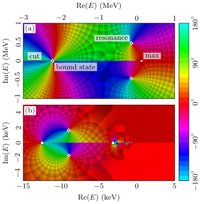
Furthermore, in contrast to , the function is holomorphic in the neighborhood of , because of the properties of the modified Coulomb functions and in the limit Gaspard and Sparenberg 2018; Gaspard 2018. Therefore, it follows from Eq. (33) that any singularity of is reflected on . In this regard, it can be shown that has two poles at , that are interpreted as the proton-proton resonance poles Kok 1980; Gaspard and Sparenberg 2018. In Fig. 6, only one of them is visible because the plot is restricted to the upper half-plane (). The other one is shown in panel (a) of Fig. 8.
The function also possesses a branch cut along the negative real semi-axis due to the logarithm in the Bethe function in Eq. (23). This branch cut makes complex at negative energy, although it is real at positive energy. Being on the boundary of the plots, the branch cut cannot be seen either in Figs. 6 or 7, but only in the top views of Fig. 8.
In addition, is responsible for the accumulation of poles and zeros shown in Fig. 7. These singularities originate from the terms in the Bethe function . The pole-zero pattern is repeated each for . Such a structure can be understood as a set of virtual states generated by the Coulomb potential between the protons.
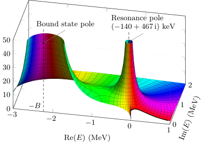
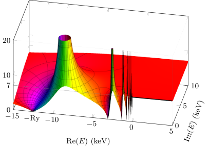
These considerations about the analytic properties of have two major consequences. First, the maximum of is directly related to the Coulomb potential. Especially, one sees in Fig. 6 that it results from a saddle point between the conjugated resonance poles and the low-energy Coulomb singularities.
Second, is not analytic at due to in Eq. (33). Therefore, its series expansion is not expected to converge over a nonzero energy range around . The common way of extracting the derivatives of would be to use polynomial extrapolation from data on a finite energy interval Schiavilla et al. 1998; Marcucci et al. 2013; *Marcucci2014a; Acharya et al. 2016. However, such a method is not accurate due to the non-negligible influence of the interval itself Acharya et al. 2016; Marcucci et al. 2013; *Marcucci2014a.
IV Zero-energy derivatives
One way to address the issue of the extrapolation to is to expand in power series directly from Eq. (33) taking advantage of the flatness of at low energy. The result (33) provides a constraint on the derivatives of with respect to the energy, especially the first derivative at zero energy: . This value plays a significant role in the proton-proton fusion at solar energies Adelberger et al. 2011. From Eq. (33), the logarithmic derivative of can be easily calculated
| (38) |
where the function has been replaced by because they share the same asymptotic expansion at . This is due to the fact that the term in Eq. (24) is negligible since all of its derivatives are zero. The first terms in the asymptotic expansion of are
| (39) |
However, it should be noted that this expansion does not converge at because of the Coulomb singularities in . It remains nevertheless valid for Gaspard and Sparenberg 2018; Baye and Brainis 2000. In addition, the expansion of the regular Coulomb integral is given by
| (40) |
Combining these results in Eq. (38), we find that the logarithmic derivative of at mostly depends on the effective-range parameters
| (41) |
The prime over refers to the derivative with respect to . This novel result was not obtained by Bahcall and May, although its numerical value is given in their paper Bahcall and May 1969. From and in Eq. (37), the result (41) yields
| (42) |
This result and all the following ones are expressed in units of MeV and fm.
It should be noted that, according to Eq. (34), and also depend on effective-range parameters. In this regard, the expansion (42) is incomplete. However, it is not possible to extract the full dependence of in the effective-range parameters since it would be necessary to modify the potential models accordingly.
Besides, one notices in Eq. (42) that the uncertainty of the effective range only slightly influences the result. Therefore, it is useful to re-express Eq. (42) in the neighborhood of with . We obtain the following result
| (43) |
around the scattering length . The central value
| (44) |
is compatible with Refs. Bahcall and May 1969; Chen et al. 2013. It turns out that the term in Eq. (41), which contains the short-range behavior of the wave functions, only contributes to about . Therefore, the uncertainty of marginally affects the overall uncertainty of , which is primarily due to the effective-range parameters and .
It is worth noting that Eq. (33) now determines all the derivatives of at . Indeed, the higher-order derivatives of are negligible in the expansion of compared to the other terms. The reason is that the derivatives of are dominated by . In particular, the second derivative of can also be calculated analytically from Eq. (33). We have
| (45) |
where the primes refer to derivatives with respect to the main variable: either for , or for . All the functions in Eq. (45) are implicitly evaluated at . It turns out that the second derivative can be neglected, as it contributes to only , far below the uncertainty of the other terms. The terms of Eq. (45) containing and its derivatives are dominating the other ones, especially the term which is about . Inserting the expansion of and at into Eq. (45), but without replacing the effective-range parameters and by their numerical value for now, we find
| (46) |
The last term in Eq. (46) comes from the term in Eq. (45). The uncertainties in this term are negligible, as it solely depends on accurately known physical quantities (, , and ).
As previously, if we focus on the neighborhood of assuming , we get from Eq. (46) the expression
| (47) |
Note that the remainder term in Eq. (47) is in unit . The central value
| (48) |
is in accordance with Ref. Chen et al. 2013. The uncertainty on is mainly due to . This result (48) is considerably more accurate than what we get from direct fitting on . In fact, the direct computation of the second derivative of depends too much on the energy interval chosen for the fitting, hence degrading its accuracy. Similar effective-range constraints can be derived for higher-order derivatives of from Eq. (33). The expected accuracy of this approach does not exceed about as it is limited by the uncertainty on .
Finally, we deduce the zero-energy derivatives of the astrophysical factor from Eqs. (43) and (47). Knowing from Eq. (7) that is proportional to , the logarithmic derivatives read Baye 2013
| (49) |
and
| (50) |
Using the values of the Fermi phase-space integral from Eq. (61), we get the results
| (51) | ||||
The central values and , obtained by setting , are compatible with Refs. Bahcall and May 1969; Adelberger et al. 2011; Chen et al. 2013; Marcucci et al. 2013; *Marcucci2014a; Angulo et al. 1999; Baye 2013. These results are obtained with an unprecedented high accuracy. In the literature, most of the uncertainties are due to the polynomial extrapolation of which is highly sensitive to the chosen energy interval Marcucci et al. 2013; *Marcucci2014a; Acharya et al. 2016. Our method is based instead on the fitting of , as suggested by the analytic structure of at low energy. Consequently, the results (51) are not affected by the uncertainty of reported for Adelberger et al. 2011.
V Conclusion
To conclude, we have derived an accurate parametrization of the energy dependence of the weak capture matrix element valid up to a few MeVs, that is based on recent effective-range functions Ramírez Suárez and Sparenberg 2017; Gaspard and Sparenberg 2018. This result provides the analytic continuation of to complex energies, and highlights the relationship between its maximum near , the broad proton-proton resonance, and the Coulomb sub-threshold singularities. In addition, it leads to a remarkably accurate determination of the logarithmic derivatives of the astrophysical factor at in terms of effective-range parameters. Our method bypasses the issue Acharya et al. 2016 of the energy-range dependence in the polynomial fitting of by means of the function , that is analytic at low energy, in contrast to . In this regard, the gain in accuracy on , , and using our method is expected to be similar if corrections, such as the two-body current terms Schiavilla et al. 1998; Park et al. 2003; Marcucci et al. 2013; *Marcucci2014a, are taken into account. Finally, the new parametrization (33) is appropriate for use in stellar and Big-Bang astrophysics as it covers a large energy range up to the binding energy of the deuteron.
Acknowledgements.
This work was supported by the European Union’s Horizon 2020 (Excellent Science) research and innovation program under Grant Agreement No. 654002.Appendix A Fermi phase-space integral
When calculating the proton-proton weak capture cross section, we are led to integrate the Dirac delta of energy-momentum conservation over the momenta of the three outgoing particles: the deuteron, the positron, and the electronic neutrino. The resulting integral is known as the Fermi phase-space integral and reads in first approximation Bahcall 1966; Wilkinson 1982; Chen et al. 2013
| (52) |
as long as the recoil of the deuteron is neglected. The released energy is found to be with the masses from Ref. Tanabashi et al. 2018. The variable in Eq. (52) is the positron energy divided by its mass. With this notation, is to be understood as the positron momentum divided by its mass. From energy conservation, the upper bound denoted as is equal to . It means that the Fermi integral also depends on the proton-proton energy . The purpose of this Appendix is to calculate the low-energy dependence of on .
The Coulomb factor in Eq. (52), accounting for the distortion of the positron wave function in the electric field of the deuteron, is given by Bahcall 1966; Wilkinson 1982; Chen et al. 2013
| (53) |
where is equal to with the fine-structure constant , and is the dimensionless radius of the deuteron. In the following calculations, we will assume Chen et al. 2013. In Eq. (53), the Sommerfeld parameter of the emitted positron must be positive, as it is repelled by the nucleus. Conversely, in a decay, the Sommerfeld parameter should take a minus sign. It should be noted that in the nonrelativistic limit (), the Coulomb distortion factor becomes
| (54) |
The Fermi integral (52) cannot be analytically calculated in a simple form. However, very efficient approximations exist. One way is to expand the Coulomb factor (53) in series of the fine-structure constant . We find
| (55) |
where is the Euler-Mascheroni constant. In this work, we limit ourselves to the order , as it is enough to obtain at least five decimal places in the final results. The same approach is followed in Ref. Wilkinson 1982 up to . Now, we just have to calculate one Fermi integral for each term in the expansion (55). The advantage is that the integrals of the form
| (56) |
which will come into play, can be expressed in terms of elementary functions for . Such expressions can be obtained by expanding the last factor in Eq. (56). The results read for
| (57) |
for
| (58) |
and for
| (59) |
We notice that, according to Eqs. (57), (58), and (59), the Fermi integral is expected to behave as at relatively large energy (). Therefore, dominates the behavior of in Eq. (7).
The factor in the logarithmic term of expansion (55) can be neglected because it remains of the order of except at large proton-proton energies (). Therefore, using Eq. (56), the Fermi integral (52) is approximated by
| (60) |
This expression allows us to find at least five decimal places without requiring numerical integration. Another advantage is the computation of the derivatives of the Fermi integrals with respect to . In this work, we need the first two derivatives of at zero proton energy (). This can be easily achieved with the derivatives of with respect to that are obtained directly from Eqs. (57), (58), and (59). The derivatives of with respect to have thus essentially the same expressions as Eq. (60) by replacing with the derivatives with respect to , denoted as . Note the change of variable in the manipulation.
The numerical values of the functions and their derivatives at , that is for , are given in Table 2. Inserting the numerical values of Table 2 in the approximation (60) for the different derivative orders () leads to the results
| (61) |
These results have also been checked by numerical integration in Wolfram Mathematica Wolfram 1999. The uncertainties in Table 2 and Eq. (61) come from the released energy . Finally, the low-energy behavior of the Fermi integral can be written as
| (62) |
with the numerical values of Eq. (61).
It should be noted that the third derivative of the Fermi function (52) with respect to is devoid of integral and can be expressed exactly in terms of . We have
| (63) |
from which the numerical value at is easily found. Our approach avoids using numerical derivatives, as they are ill-conditioned in finite precision arithmetic, especially for high-order derivatives. This also ensures the accuracy of the results (61).
Appendix B Laplace transforms of the modified Coulomb functions
In this Appendix, we present the derivation of the Laplace transforms of the modified Coulomb wave functions and defined in Ref. Gaspard 2018. More explicitly, we are looking for analytical expressions of the integrals
| (64) |
and
| (65) |
where is the dimensionless radial coordinate, and is the dimensionless wave number. Although we only need the result for , we have made our derivation more general. The reason is that we use the connection formula between and developed in Ref. Gaspard 2018 to calculate on the basis of for any integer .
B.1 Regular Coulomb integral
As shown in Ref. Gaspard 2018, the Coulomb function in Eq. (64) is given by
| (66) |
where , and is the Bahcall and May constant Bahcall and May 1969. The regularized confluent hypergeometric function in Eq. (66) is defined by the series Olver et al. 2010
| (67) |
where is the Pochhammer symbol. The division by in Eq. (67) eliminates the singularities of at Olver et al. 2010. Using the definition (66), the regular Coulomb integral (64) expands as follows
| (68) |
All the remaining integrals in Eq. (68) are given by
| (69) |
One notices that the combination of Eqs. (68) and (69) leads to the Gauss hypergeometric function , or more specifically to its regularized version Olver et al. 2010
| (70) |
Using the definition (70) in Eq. (68), we obtain the following result:
| (71) |
Remarkably, this result is considerably simplified in the special case . Indeed, the hypergeometric function in Eq. (71) is then of the form , which reduces to Olver et al. 2010 because of the simplification in the series (70). From Eq. (71), one finds
| (72) |
This useful result is at the basis of the parametrization of proposed in this paper.
B.2 Irregular Coulomb integral
Now, we calculate the Laplace transform (65) of . This calculation is significantly less straightforward than for , because it does not reduce to elementary functions for . The Coulomb function is defined in Ref. Gaspard 2018 as
| (73) |
where the choice of the upper or lower sign is immaterial. In Eq. (73), is the Tricomi confluent hypergeometric function, and the Bethe functions are defined as
| (74) |
The subtraction by in Eq. (73) is intended to compensate for the singularities of in the complex plane of the energy. This operation makes regular for Gaspard 2018.
Performing the direct integration of Eq. (73) by means of the integral representation of Olver et al. 2010 leads to
| (75) |
Note that, this function is not finite for partial waves higher than () due to the vertical asymptote of at . When , the hypergeometric function in the above equation can be efficiently computed from its continued fraction expansion.
The expression (75) is quite difficult to analyze at low energy because the hypergeometric function shows an essential singularity at . Although this singularity is compensated by , it prevents the hypergeometric function from having a convergent low-energy expansion. This is why we propose to determine a suitable approximation to Eq. (75) from another approach.
It turns out that the function is related to the regular Coulomb function . We have shown in Ref. Gaspard 2018 that obeys the following connection formula
| (76) |
where the dots refer to derivatives with respect to . This useful property is preserved by the Laplace transforms (64) and (65). Therefore, the function can be calculated from derivatives of as follows Gaspard 2018
| (77) |
However, in order to calculate the derivatives in Eq. (77), we need to use the general expression (71) valid of for all . In this regard, we have found convenient to approximate the hypergeometric function by its low-energy confluent limit
| (78) |
The approximation (78) could be improved at by the confluence expansion (20a) in Ref. Nagel 2004. However, this expansion converges so slowly for that we will not use it here. The advantage of the approximation (78) is the consistency with Bahcall’s and May’s results in the zero-energy limit. It is useful in our calculation to rewrite the confluent hypergeometric function in Eq. (78) in terms of the regular Coulomb function
| (79) |
The approximation of for is thus given by
| (80) |
From Eq. (71) to Eq. (80), we have taken the modulus of the factor because should still remain a positive real function after the approximation (78). The logarithmic derivative of with respect to can be easily calculated from Eq. (80):
| (81) |
We neglect the logarithmic term in Eq. (81) because it is irrelevant in the approximation of Eq. (78). Combining two expressions (81) evaluated at and in Eq. (77), we get
| (82) |
This relation can be simplified further by means of the definition (73) of with the plus sign. Finally, after the elimination of the digamma functions with Eq. (74), we obtain
| (83) |
In the special case of interest , this result can be written as
| (84) |
where is the upper incomplete gamma function defined by
| (85) |
When and , the ratio (84) evaluates to about . The incomplete gamma function in Eq. (84) can also be related to the exponential integral as done in Bahcall’s and May’s work Bahcall and May 1969:
| (86) |
Bahcall, however, limited his calculation to zero energy, in contrast to the property (84) valid up to a few MeVs.
Furthermore, the novel result (84) means that is nearly proportional to on a large energy range. The accuracy of this property is graphically tested in Fig. 9. As we can see, the relative error of the estimate at , that corresponds to , is only . The overall accuracy of the approximation (84) over a few MeVs is primarily due to the smallness of with respect to (). In fact, it can be shown that both and have the same neutral-charge limit:
| (87) |
Therefore, the property (84) tends to be exact for , but also for . These observations have important consequences in the parametrization of the weak capture matrix element .
References
- Bethe and Critchfield (1938) H. A. Bethe and C. L. Critchfield, Phys. Rev. 54, 248 (1938).
- Salpeter (1952) E. E. Salpeter, Phys. Rev. 88, 547 (1952).
- Bahcall and May (1969) J. N. Bahcall and R. M. May, Astrophys. J. 155, 501 (1969).
- Bahcall and Pinsonneault (1992) J. N. Bahcall and M. H. Pinsonneault, Rev. Mod. Phys. 64, 885 (1992).
- Kamionkowski and Bahcall (1994) M. Kamionkowski and J. N. Bahcall, Astrophys. J. 420, 884 (1994).
- Kong and Ravndal (2001) X. Kong and F. Ravndal, Phys. Rev. C 64, 044002 (2001).
- Ando et al. (2008) S. Ando, J. W. Shin, C. H. Hyun, S. W. Hong, and K. Kubodera, Phys. Lett. B 668, 187 (2008).
- Butler and Chen (2001) M. Butler and J.-W. Chen, Phys. Lett. B 520, 87 (2001).
- Carlson et al. (1991) J. Carlson, D. O. Riska, R. Schiavilla, and R. B. Wiringa, Phys. Rev. C 44, 619 (1991).
- Park et al. (2003) T.-S. Park, L. E. Marcucci, R. Schiavilla, M. Viviani, A. Kievsky, S. Rosati, K. Kubodera, D.-P. Min, and M. Rho, Phys. Rev. C 67, 055206 (2003).
- Schiavilla et al. (1998) R. Schiavilla, V. G. J. Stoks, W. Glöckle, H. Kamada, A. Nogga, J. Carlson, R. Machleidt, V. R. Pandharipande, R. B. Wiringa, et al., Phys. Rev. C 58, 1263 (1998).
- Marcucci et al. (2013) L. E. Marcucci, R. Schiavilla, and M. Viviani, Phys. Rev. Lett. 110, 192503 (2013).
- Marcucci (2014) L. E. Marcucci, J. Phys.: Conf. Ser. 527, 012023 (2014).
- Adelberger et al. (2011) E. G. Adelberger, A. García, R. G. Hamish Robertson, K. A. Snover, A. B. Balantekin, K. Heeger, M. J. Ramsey-Musolf, D. Bemmerer, A. Junghans, et al., Rev. Mod. Phys. 83, 195 (2011).
- Chen et al. (2013) J.-W. Chen, C.-P. Liu, and S.-H. Yu, Phys. Lett. B 720, 385 (2013).
- Acharya et al. (2016) B. Acharya, B. D. Carlsson, A. Ekström, C. Forssén, and L. Platter, Phys. Lett. B 760, 584 (2016).
- Kok (1980) L. P. Kok, Phys. Rev. Lett. 45, 427 (1980).
- Tanabashi et al. (2018) M. Tanabashi, K. Hagiwara, K. Hikasa, K. Nakamura, Y. Sumino, F. Takahashi, J. Tanaka, K. Agashe, G. Aielli, et al. (Particle Data Group), Phys. Rev. D 98, 030001 (2018).
- Gaspard and Sparenberg (2018) D. Gaspard and J.-M. Sparenberg, Phys. Rev. C 97, 044003 (2018).
- Ramírez Suárez and Sparenberg (2017) O. L. Ramírez Suárez and J.-M. Sparenberg, Phys. Rev. C 96, 034601 (2017).
- Baye and Brainis (2000) D. Baye and E. Brainis, Phys. Rev. C 61, 025801 (2000).
- Blokhintsev et al. (2017) L. D. Blokhintsev, A. S. Kadyrov, A. M. Mukhamedzhanov, and D. A. Savin, Phys. Rev. C 95, 044618 (2017).
- Blokhintsev et al. (2018a) L. D. Blokhintsev, A. S. Kadyrov, A. M. Mukhamedzhanov, and D. A. Savin, Phys. Rev. C 97, 024602 (2018a).
- Blokhintsev et al. (2018b) L. D. Blokhintsev, A. S. Kadyrov, A. M. Mukhamedzhanov, and D. A. Savin, Phys. Rev. C 98, 064610 (2018b).
- Wiringa et al. (1995) R. B. Wiringa, V. G. J. Stoks, and R. Schiavilla, Phys. Rev. C 51, 38 (1995).
- Stoks et al. (1994) V. G. J. Stoks, R. A. M. Klomp, C. P. F. Terheggen, and J. J. de Swart, Phys. Rev. C 49, 2950 (1994).
- Baye (2013) D. Baye, in The Universe Evolution: Astrophysical and Nuclear Aspects, Physics Research and Technology, edited by I. Strakovsky and L. D. Blokhintsev (Nova Science Pub. Inc., Hauppauge, NY, 2013) Chap. 5, pp. 185–216.
- Acharya et al. (2019) B. Acharya, L. Platter, and G. Rupak, Phys. Rev. C 100, 021001 (2019).
- Olver et al. (2010) F. W. J. Olver, D. W. Lozier, R. F. Boisvert, and C. W. Clark, NIST Handbook of Mathematical Functions, 1st ed. (NIST, New York, 2010).
- Moravcsik (1958) M. J. Moravcsik, Nucl. Phys. 7, 113 (1958).
- Kottler and Kowalski (1964) H. Kottler and K. L. Kowalski, Nucl. Phys. 53, 334 (1964).
- McGee (1966) I. J. McGee, Phys. Rev. 151, 772 (1966).
- Humberston and Wallace (1970) J. W. Humberston and J. B. G. Wallace, Nucl. Phys. A 141, 362 (1970).
- Oteo (1988) J. A. Oteo, Can. J. Phys. 66, 478 (1988).
- Gaspard (2018) D. Gaspard, J. Math. Phys. 59, 112104 (2018).
- Bethe (1949) H. A. Bethe, Phys. Rev. 76, 38 (1949).
- Hamilton et al. (1973) J. Hamilton, I. Øverbö, and B. Tromborg, Nucl. Phys. B 60, 443 (1973).
- Machleidt (2001) R. Machleidt, Phys. Rev. C 63, 024001 (2001).
- Rupak and Ravi (2015) G. Rupak and P. Ravi, Phys. Lett. B 741, 301 (2015).
- Kurylov et al. (2002) A. Kurylov, M. J. Ramsey-Musolf, and P. Vogel, Phys. Rev. C 65, 055501 (2002).
- Kurylov et al. (2003) A. Kurylov, M. J. Ramsey-Musolf, and P. Vogel, Phys. Rev. C 67, 035502 (2003).
- Wegert (2012) E. Wegert, Visual Complex Functions: An Introduction with Phase Portraits (Birkhäuser, Basel, 2012).
- Angulo et al. (1999) C. Angulo, M. Arnould, M. Rayet, P. Descouvemont, D. Baye, C. Leclercq-Willain, A. Coc, S. Barhoumi, P. Aguer, et al., Nucl. Phys. A 656, 3 (1999).
- Bahcall (1966) J. N. Bahcall, Nucl. Phys. 75, 10 (1966).
- Wilkinson (1982) D. H. Wilkinson, Nucl. Phys. A 377, 474 (1982).
- Wolfram (1999) S. Wolfram, The Mathematica® Book, 4th ed. (Cambridge University, New York, 1999).
- Nagel (2004) B. Nagel, J. Math. Phys. 45, 495 (2004).