Neural Network Attributions: A Causal Perspective
Abstract
We propose a new attribution method for neural networks developed using first principles of causality (to the best of our knowledge, the first such). The neural network architecture is viewed as a Structural Causal Model, and a methodology to compute the causal effect of each feature on the output is presented. With reasonable assumptions on the causal structure of the input data, we propose algorithms to efficiently compute the causal effects, as well as scale the approach to data with large dimensionality. We also show how this method can be used for recurrent neural networks. We report experimental results on both simulated and real datasets showcasing the promise and usefulness of the proposed algorithm.
marginparsep has been altered.
topmargin has been altered.
marginparwidth has been altered.
marginparpush has been altered.
The page layout violates the ICML style.
Please do not change the page layout, or include packages like geometry, savetrees, or fullpage, which change it for you.
We’re not able to reliably undo arbitrary changes to the style. Please remove the offending package(s), or layout-changing commands and try again.
1 Introduction
Over the last decade, deep learning models have been highly successful in solving complex problems in various fields ranging from vision, speech to more core fields such as chemistry and physics (Deng et al. 2014; Sadowski et al. 2014; Gilmer et al. 2017). However, a key bottleneck in accepting such models in real-life applications, especially risk-sensitive ones, is the “interpretability problem”. Usually, these models are treated as black boxes without any knowledge of their internal workings. This makes troubleshooting difficult in case of erroneous behaviour. Moreover, these algorithms are trained on a limited amount of data which most often is different from real-world data. Artifacts that creep into the training dataset due to human error or unwarranted correlations in data creation have an adverse effect on the hypothesis learned by these models. If treated as black boxes, there is no way of knowing whether the model actually learned a concept or a high accuracy was just fortuitous. This limitation of black-box deep learned models has paved way for a new paradigm, “explainable machine learning”.
While the field is nascent, several broad approaches have emerged (Simonyan et al. 2013; Yosinski et al. 2015; Frosst & Hinton 2017; Letham et al. 2015), each having its own perspective to explainable machine learning. In this work, we focus on a class of interpretability algorithms called “attribution-based methods”. Formally, attributions are defined as the effect of an input feature on the prediction function’s output (Sundararajan et al. 2017). This is an inherently causal question, which motivates this work. Current approaches involve backpropagating the signals to input to decipher input-output relations (Sundararajan et al. 2017; Selvaraju et al. 2016; Bach et al. 2015; Ribeiro et al. 2016) or approximating the local decision boundary (around the input data point in question) via “interpretable” regressors like linear classifiers (Ribeiro et al. 2016; Selvaraju et al. 2016; Zhou & Troyanskaya 2015; Alvarez-Melis & Jaakkola 2017) or decision trees.
In the former category of methods, while gradients answer the question “How much would perturbing a particular input affect the output?”, they do not capture the causal influence of an input on a particular output neuron. The latter category of methods that rely on “interpretable” regression is also prone to artifacts as regression primarily maps correlations rather than causation. In this work, we propose a neural network attribution methodology built from first principles of causality. To the best of our knowledge, while neural networks have been modeled as causal graphs (Kocaoglu et al. 2017), this is the first effort on a causal approach to attribution in neural networks.
Our approach views the neural network as a Structural Causal Model (SCM), and proposes a new method to compute the Average Causal Effect of an input neuron on an output neuron. Using standard principles of causality to make the problem tractable, this approach induces a setting where input neurons are not causally related to each other, but can be jointly caused by a latent confounder (say, data-generating mechanisms). This setting is valid in many application domains that use neural networks, including images where neighboring pixels are often affected jointly by a latent confounder, rather than direct causal influence (a “doer” can take a paint brush and oddly color a certain part of an image, and the neighboring pixels need not change). We first show our approach on a feedforward network, and then show how the proposed methodology can be extended to Recurrent Neural Networks which may violate this setting. We also propose an approximate computation strategy that makes our method viable for data with large dimensionality. We note that our work is different from a related subfield of structure learning (Eberhardt 2007; Hoyer et al. 2009; Hyttinen et al. 2013; Kocaoglu et al. 2017), where the goal is to discern the causal structure in given data (for example, does feature cause feature or vice versa?). The objective of our work is to identify the causal influence of an input on a learned function’s (neural network’s) output.
Our key contributions can be summarized as follows. We propose a new methodology to compute causal attribution in neural networks from first principles; such an approach has not been expounded for neural network attribution so far to the best of our knowledge. We introduce causal regressors for better estimates of the causal effect in our methodology, as well as to provide a global perspective to causal effect. We provide a strategy to scale the proposed method to high-dimensional data. We show how the proposed method can be extended to Recurrent Neural Networks. We finally present empirical results to show the usefulness of this methodology, as well as compare it to a state-of-the-art gradient-based method to demonstrate its utility.
2 Prior Work and Motivation
Attribution methods for explaining deep neural networks deal with identifying the effect of an input neuron on a specific output neuron. The last few years have seen a growth in research efforts in this direction (Sundararajan et al. 2017; Smilkov et al. 2017; Shrikumar et al. 2017; Montavon et al. 2017; Bach et al. 2015). Most such methods generate ‘saliency maps’ conditioned on the given input data, where the map captures the contribution of a feature towards the overall function value. Initial attempts involved perturbing regions of the input via occlusion maps (Zeiler & Fergus 2014; Zhou & Troyanskaya 2015) or inspecting the gradients of an output neuron with respect to an input neuron (Simonyan et al. 2013). However, the non-identifiability of “source of error” has been a central impediment to designing attribution algorithms for black box deep models. It is impossible to distinguish whether an erroneous heatmap (given our domain knowledge) is an artifact of the attribution method or a consequence of poor representations learnt by the network (Sundararajan et al. 2017).
In order to analyze attribution methods in a uniform manner, newer methods (Sundararajan et al. 2017) have spelt out axioms that can be used to evaluate a given method: (i) Conservativeness (Bach et al. 2015), (ii) Sensitivity, (iii) Implementation invariance, (iv) Symmetry preservation (Sundararajan et al. 2017), and (v) Input invariance (Kindermans et al. 2017). Methods that use the infinitesimal approximation of gradients and local perturbations violate axiom (ii). In flatter regions of the learned neural function, perturbing input features or investigating gradients might falsely point to zero attributions to these features.
From a causal point of view, both gradient- and perturbation-based methods can be viewed as special instances of Individual Causal Effect (ICE), defined as, . denotes the output of the network for a given individual input vector , with an arbitrary neuron set to . represents the network output without any intervention. If input neurons are assumed to not cause each other, then calculating by setting to can be related to taking the partial derivative, i.e., where . Complex inter-feature interactions can conceal the real importance of input feature , when only the ICE is analyzed. Appendix A.2 provides more details of this observation.
Subsequent methods like DeepLIFT (Shrikumar et al. 2017) and LRP (Bach et al. 2015) solved the sensitivity issue by defining an appropriate baseline and approximating the instantaneous gradients with discrete differences. This however, breaks axiom (iii), as unlike gradients, discrete gradients do not follow the chain rule (Shrikumar et al. 2017). Integrated Gradients (Sundararajan et al. 2017) extended this method to include actual gradients and averaged them out along a path from the baseline to the input vector. This method is perhaps closest to capturing causal influences since it satisfies most axioms among similar methods (and we use this for empirical comparisons in this work). Nevertheless, this method does not marginalize over other input neurons and the attributions may thus still be biased.
Implicit biases in current attribution methods:
Kindermans et al. (Kindermans et al. 2017) showed that almost all attribution methods are sensitive to even a simple constant shift of all the input vectors. This implicitly means that the attributions generated for every input neuron are biased by the values of other input neurons for a particular input data. To further elucidate this point, consider a function . Let the baseline be . Consider two input vectors and . The Integrated Gradients method (which unlike other methods, satisfies all the axioms in Section 2 except axiom (v)) assigns attributions to as for input and for input . This result is misleading, because both input vectors have exactly the same baseline and same value for feature , but the attribution algorithm assigns different values to it. However, because the form of the function is known a priori, it is clear that both and have equal causal strengths towards affecting , and in this particular scenario, the entire change in is due to interventions on and not .
In this work, we propose a causal approach to attribution, which helps supersede the implicit biases in current methods by marginalizing over all other input parameters. We show in Section 4, after our definitions, that our approach to causal attribution satisfies all axioms, with the exception of axiom (i), which is not relevant in a causal setting. Besides, via the use of causal regressors 4.3, a global perspective of the deep model can be obtained, which is not possible by any existing attribution method.
The work closest to ours is a recent effort to use causality to explain deep networks in natural language processing (Alvarez-Melis & Jaakkola 2017). This work is a generalization of LIME (Ribeiro et al. 2016), where the idea is to infer dependencies via regularized linear regression using perturbed samples local to a particular input. Analyzing the weights of this learned function provides insights into the network’s local behavior. However, regression only learns correlations in data which could be markedly different from causation. Other efforts such as (Alvarez-Melis & Jaakkola 2018; Li et al. 2018) attempt to explain in terms of latent concepts, which again do not view effect from a causal perspective, which is the focus of this work. More discussion of prior work is presented in Appendix A.2.
3 Background: Neural Networks as Structural Causal Models (SCMs)
This work is founded on principles of causality, in particular Structural Causal Models (SCMs) and the calculus, as in (Pearl 2009). A brief exposition on the concepts used in this work is provided in Appendix A.1.
We begin by stating that neural network architectures can be trivially interpreted as SCMs (as shown in other recent work such as (Kocaoglu et al. 2017)). Note that we do not explicitly attempt to find the causal direction in this case, but only identify the causal relationships given a learned function.

Figure 1a depicts such a feedforward neural network architecture. Neural networks can be interpreted as directed acyclic graphs with directed edges from a lower layer to the layer above. The final output is thus based on a hierarchy of interactions between lower level nodes.
Proposition 1.
An -layer feedforward neural network where is the set of neurons in layer has a corresponding SCM , where is the input layer and is the output layer. Corresponding to every , refers to the set of causal functions for neurons in layer . refers to a set of exogenous random variables which act as causal factors for the input neurons .
Appendix A.3.1 contains a simple proof of Proposition 1. In practice, only the neurons in layer and layer are observables, which are derived from training data as inputs and outputs respectively. The causal structure can hence be reduced to SCM by marginalizing out the hidden neurons.
Corollary 1.1.
Every -layer feedforward neural network , with denoting the set of neurons in layer , has a corresponding SCM which can be reduced to an SCM .
Appendix A.3.2 contains a formal proof for Corollary 1.1. Marginalizing the hidden neurons out by recursive substitution (Corollary 1.1) is analogous to deleting the edges connecting these nodes and creating new directed edges from the parents of the deleted neurons to their respective child vertices (the neurons in the output layer) in the corresponding causal Bayesian network. Figure 1a illustrates an example of a 3-layer neural network (the left figure) with 1 input, 1 hidden and 1 output layer (W.l.o.g); after marginalizing out the hidden layer neurons, the reduced causal Bayesian network on the right is obtained.
Recurrent Neural Networks (RNNs):
Defining an SCM directly on a more complex neural network architecture such as RNNs would introduce feedback loops and the corresponding causal Bayesian network is no longer acyclic. Cyclic SCMs may be ambiguous and not register a unique probability distribution over its endogenous variables (Bongers et al. 2016). Proposition 1, however, holds for a time-unfolded RNN; but care must be taken in defining the reduced SCM from the original SCM . Due to the recurrent connections between hidden states, marginalizing over the hidden neurons (via recursive substitution) creates directed edges from input neurons at every timestep to output neurons at subsequent timesteps. In tasks such as sequence prediction, where the output neuron at time is taken as the input at time , the assumption that input neurons are not causally related is violated. We discuss this in detail in Section 4.5. Figure 1b depicts our marginalization process in RNNs. W.l.o.g., we consider a single hidden layer unfolded recurrent model where the outputs are used as inputs for the next time step. The shaded vertices are the hidden layer random variables, refers to the output at time and refers to the input at time . In the original SCM (left figure), vertex causes (there exists a functional dependence). If is marginalized out, its parents and become the causes (parents) of . Similarly, if is marginalized out, both and become causes of . Using similar reasoning, the reduced (marginalized) SCM on the right is obtained.
4 Causal Attributions for Neural Networks
4.1 Causal Attributions
This work attempts to address the question: ”What is the causal effect of a particular input neuron on a particular output neuron of the network?”. This is also known in literature as the “attribution problem” (Sundararajan et al. 2017). We seek the information required to answer this question as encapsulated in the SCM consistent with the neural model architecture .
Definition 4.1.
(Average Causal Effect). The Average Causal Effect (ACE) of a binary random variable on another random variable is commonly defined as .
While the above definition is for binary-valued random variables, the domain of the function learnt by neural networks is usually continuous. Given a neural network with input and output , we hence measure the of an input feature with value on an output feature as:
| (1) |
Definition 4.2.
(Causal Attribution). We define as the causal attribution of input neuron for an output neuron .
Note that the gradient is sometimes used to approximate the Average Causal Effect () when the domain is continuous (Peters et al. 2017). However, as mentioned earlier, gradients suffer from sensitivity and induce causal effects biased by other input features. Also, it is trivial to see that our definition of causal attributions satisfy axioms (ii) - (vi) (as in Section 2), with the exception of axiom (i). According to axiom (i), is conservative if , where is a vector of attributions for the input. However, our method identifies the causal strength of various input features towards a particular output neuron and not a linear approximation of a deep network, so it’s not necessary for the causal effects to add up to the difference between and . Axiom (ii) is satisfied due to the consideration of a reference baseline value. Axioms (iii) and (iv) hold because we directly calculate the interventional expectations which do not depend on the implementation as long as it maps to an equivalence function. (Kindermans et al. 2017) show that most attribution algorithms are very sensitive to constant shifts in the input. In the proposed method, if two functions , where is the constant shift, the respective causal attributions of and stay exactly the same. Thus, our method also satisfies axiom (v).
In Equation 1, an ideal baseline would be any point along the decision boundary of the neural network, where predictions are neutral. However, (Kindermans et al. 2017) showed that when a reference baseline is fixed to a specific value (such as a zero vector), attribution methods are not affine-invariant. In this work, we propose the average ACE of on as the baseline value for , i.e. . In absence of any prior information, we assume that the “doer” is equally likely to perturb to any value between , i.e. , where is the domain of . While we use the uniform distribution, which represents the maximum entropy distribution among all continuous distributions in a given interval, if more information about the distribution of interventions performed by the “external” doer is known, this could be incorporated instead of an uniform distribution. Domain knowledge could also be incorporated to select a significant point as the baseline. The would then be .Our choice of baseline in this work is unbiased and adaptive. Another rationale behind this choice is that represents the expected value of random variable when the random variable is set to . If the expected value of is constant for all possible interventional values of , then the causal effect of on would be for any value of . The baseline value in that case would also be the same constant, resulting in .
4.2 Calculating Interventional Expectations
We refer to as the interventional expectation of given the intervention . By definition:
| (2) |
Naively, evaluating Equation 2 would involve sampling all other input features from the empirical distribution keeping feature , and then averaging the output values. Note, this assumes that the input features don’t cause one another. However, due to the curse of dimensionality, this unbiased estimate of would have a high variance. Moreover, running through the entire training data for each interventional query would be time-consuming. We hence propose an alternative mechanism to compute the interventional expectations.
Consider an output neuron in the reduced SCM , obtained by marginalizing out the hidden neurons in a given neural network (Corollary 1.1). The causal mechanism can be written as , where refers to neuron in the input layer, and is the number of input neurons. If we perform a operation on the network, the causal mechanism is given by . For brevity, we drop the subscript and simply refer to this as . Let . Since is a neural network, it is smooth (assuming smooth activation functions). Now, the second-order Taylor’s expansion of the causal mechanism around the vector is given by (recall is the vector of input neurons):
| (3) |
Taking expectation on both sides (marginalizing over all other input neurons):
| (4) |
The first-order terms vanish because . We now only need to calculate the individual interventional means and, the interventional covariance between input features to compute Equation 2. Such approximations of deep non-linear neural networks via Taylor’s expansion have been explored before in the context of explainability (Montavon et al. 2017), though their overall goal was different.
While every SCM , obtained via marginalizing out the hidden neurons, registers a causal Bayesian network, this network is not necessarily causally sufficient (Reichenbach’s common cause principle) (Pearl 2009). There may exist latent factors or noise which jointly cause the input features, i.e., the input features need not be independent of each other. We hence propose the following.
Proposition 2.
Given an -layer feedforward neural network with denoting the set of neurons in layer and its corresponding reduced SCM , the intervened input neuron is d-separated from all other input neurons.
Corollary 2.1.
Given an -layer feedforward neural network with denoting the set of neurons in layer and an intervention on neuron , the probability distribution of all other input neurons does not change, i.e. and .
The proof of Corollary 2.1 is rather trivial and directly follows from Proposition 2 and d-seperation (Pearl 2009). Thus, the interventional means and covariances are equal to the observational means and covariances respectively. The only intricacy involved now is in the means and covariances related to the intervened input neuron . Since , these can be computed as and (the input layer).
In other words, Proposition 2 and Corollary 2.1 induce a setting where causal dependencies (functions) do not exist between different input neurons. This assumption is often made in machine learning models (where methods like Principal Component Analysis are applied if required to remove any correlation between the input dimensions). If there was a dependence between input neurons, that is due to latent confounding factors (nature) and not the causal effect of one input on the other. Our work is situated in this setting. This assumption is however violated in the case of time-series models or sequence prediction tasks, which we handle later in Section 4.5.
4.3 Computing ACE using Causal Regressors
The ACE (Eqn 1) requires the computation of two quantities: the interventional expectation and the baseline. We defined the baseline value for each input neuron to be . In practice, we evaluate the baseline by perturbing the input neuron uniformly in fixed intervals from [], and computing the interventional expectation.
The interventional expectation is a function of as all other variables are marginalized out. In our implementations, we assume this function to be a member of the polynomial class of functions (this worked well for our empirical studies, but can be replaced by other classes of functions if required). Bayesian model selection (Claeskens et al. 2008) is employed to determine the optimal order of the polynomial that best fits the given data by maximizing the marginal likelihood. The prior in Bayesian techniques guard against overfitting in higher order polynomials. can then be easily computed via analytic integration using the predictive mean as the coefficients of the learned polynomial model. The predictive variance of at any point gives an estimate of the model’s confidence in its decision. If the variance is too high, more sampling of the interventional expectation at different values may be required. For more details, we urge interested readers to refer to (Christopher 2016)[Chap 3]. We name the learned polynomial functions causal regressors. can thus be obtained by evaluating the causal regressor at and subtracting this value from the . Calculating interventional expectations for multiple input values is a costly operation; learning causal regressors allows one to estimate these values on-the-fly for subsequent attribution analysis. Note that other regression techniques like spline regression can also be employed to learn the interventional expectations. In this work, the polynomial class of functions was selected for its mathematical simplicity.
4.4 Overall Methodology
We now summarize our overall methodology to compute causal attributions of a given input neuron for a particular output neuron in a feedforward neural network (Defn 4.2). Phase I of our method computes the interventional expectations (Sec 4.2) and Phase II learns the causal regressors and estimates the baseline (Sec 4.3).
Phase I:
For feedforward networks, the calculation of interventional expectations is straightforward. The empirical means and covariances between input neurons can be precomputed from training data (Corollary 2.1). Eqn 4 is computed using these empirical estimates to obtain the interventional expectations, , for different values of . Appendix A.4.1 presents a detailed algorithm/pseudocode along with its complexity analysis. In short, for different interventional values and input neurons, the algorithmic complexity of Phase I for feedforward networks would be O().
Phase II:
As highlighted earlier, calculating interventional expectations can be costly; so, we learn a causal regressor function that can approximate this expectation for subsequent on-the-fly computation of interventional expectations. The output of Phase I (interventional expectations at different interventions on ) is used as training data for the polynomial class of functions (Sec 4.3). The causal regressors are learned using Bayesian linear regression, and the learned model is used to provide the interventional expectations for out-of-sample interventions. Appendix A.4.3 presents a detailed algorithm.
4.5 Causal Attribution in RNNs
As mentioned before, the setting where causal dependencies do not exist between different input neurons is violated in the case of RNNs. In the corresponding causally sufficient Bayesian network for a recurrent architecture, input neurons are not independent from after an intervention on as they are d-connected (Pearl 2009) (see Figure 1b). For a recurrent neural network(RNN), if it does not have output to input connections, then the unfolded network can be given the same treatment as feedforward networks for calculating . However, in the presence of recurrent connections from output to input layers, the probability distribution of the input neurons at subsequent timesteps would change after an intervention on neuron ( input feature at time ). As a result, we cannot precompute the empirical covariance and means for use in Equation 4. In such a scenario, means and covariances are estimated after evaluating the RNN over each input sequence in the training data with the value at . This ensures that these empirical estimates are calculated from the interventional distribution . Eqn 4 is then evaluated to obtain the interventional expectations. Appendix A.4.2 presents a detailed algorithm/pseudocode. The complexity per input neuron is O(), with training samples and interventional values. The overall complexity scales linearly with the timelag for causal attributions for a particular output at timestep .
Proposition 3.
Given a recurrent neural function, unfolded in the temporal dimension, the output at time will be “strongly” dependent on inputs from timesteps to , where .
We present the proof for Proposition 3 in Appendix A.3.4. can be easily computed per sample with a single backward pass over the computational graph. This reduces the complexity of understanding causal attributions of all features for a particular output at time from O(n.num.t.k) to O(n.num..k). Here is the number of input neurons at each time-step.
4.6 Scaling to Large Data
Evaluating the interventional expectations using Eqn 4 involves calculating the Hessian. Note however that we never explicitly require the Hessian, just the term . We provide an efficient methodology to compute the interventional expectations for high-dimensional data, using the Taylor series expansion of around and the eigendecomposition of . This allowed us to get results significantly faster than exact calculations (0.04s for the approximation v/s 3.04s per computation for experiments on MNIST dataset with a deep neural network of 4 hidden layers). More details are provided in Appendix A.5.
5 Experiments and Results
The implementation of our method is publicly available at https://github.com/Piyushi-0/ACE.
5.1 Iris dataset
A 3-layer neural network (with relu() activation functions) was trained on the Iris dataset (Dheeru & Karra Taniskidou 2017). All the input features were [0-1] normalized. Fig 2 shows how our method provides a powerful tool for deciphering neural decisions at an individual feature level. Figs 2 a, b & c depict causal regressors for the three classes and all four features. These plots easily reveal that smaller petal length and width are positively causal () for Iris-setosa class; moderate values can be attributed to Iris-versicolor; and higher values favor the neural decision towards Iris-verginica. Due to the simplicity of the data, it can be almost accurately separated with axis-aligned decision boundaries. Fig 2d, shows the structure of the learned decision tree. PW refers to the feature petal width. The yellow colored sections in Figs 2a, b and c are the regions where the decision tree predicts the corresponding class by thresholding the petal width value. In all three figures, the causal regressors show strong positive ACE of petal width for the respective classes. Figs 2 e and f are scatter plots for sepal width and petal width respectively for all the three classes. Figure 2f clearly shows that (in accordance with the inference from Figs 2a, b and c). Interestingly, the trend is reversed for sepal width, which has also been identified by the neural network as evident from Figs 2a and c. Note that such a global perspective on explaining neural networks is not possible with any other attribution method.

5.2 Simulated data

Our approach can also help in generating local attributions just like other contemporary attribution algorithms. Causal attributions of each input neuron for output with ( refers to the input vector value at neuron ), can be used as a saliency map to explain the local decisions. The simulated dataset is generated following a similar procedure used in the original LSTM paper (Hochreiter & Schmidhuber 1997) (procedure described in Appendix A.6.1). Only the first three features of a long sequence is relevant for the class label of that sequence. A Gated Recurrent Unit (GRU) with a single input, hidden and output neuron with sigmoid() activations is used to learn the pattern. The trained network achieves an accuracy of . We compared the saliency maps generated by our method with Integrated Gradients (IG) (Sundararajan et al. 2017) because it is the only attribution method that satisfies all the axioms, except axiom (v) (Section 2). The saliency maps were thresholded to depict only positive contributions. Figures 3a and b show the results.
By construction, the true recurrent function should consider only the first three features as causal for class prediction. While both IG and causal attributions associate positive values to the first two features, a attribution for the third feature (in Fig 3a) might seem like an error of the proposed method. A closer inspection however reveals that the GRU does not even look at the third feature before assigning a label to a sequence. From the simulated test dataset, we created three separate datasets by imputing the feature as , . Each was then passed through the GRU and the average test error was calculated. The results in Fig 3c indicate that the third feature was never considered by the learned model for classifying the input patterns. While imputing and changed the LSTM’s prediction and times respectively, when evaluated over 1M sequences, imputing had no effect. IG heatmaps (Fig 3b) did not detect this due to biases induced by strong correlations between input features.
5.3 Airplane Data

We used a publicly available NASA Dashlink flight dataset (https://c3.nasa.gov/dashlink/projects/85/) to train a single hidden layer LSTM. The LSTM learns the flight’s trajectory, with outputs used as inputs in the next timestep. The optimal lag-time was determined to be (Proposition 3). Given a flight trajectory, to compute , we intervene on the LSTM by simulating the trajectory with for all trajectories in the train set (all input features are taken from train set). The interventional means and covariances are then computed from these simulated trajectories and used in Eqn 4 (See Algorithm 2 in the Appendix). Fig 4a depicts the results for a specific flight, which was deemed as an anomaly by the Flight Data Recorder (FDR) report (due to slippery runway, the pilot could not apply timely brakes, resulting in a steep acceleration in the airplane post-touchdown). Observing the causal attributions for the lateral acceleration (LATG) parameter seconds post-touchdown shows strong causal effects in the Lateral acceleration (LATG), Longitudinal acceleration (LONG), Pitch (PTCH) and Roll (ROLL) parameters of the flight sequence up to 7 seconds before. These results strongly agree with the FDR report. For comparison, Fig 4b shows the causal attributions for a normal flight which shows no specific structure in its saliency maps. Figs 4 c and d show explanations generated for the same two flights using the IG method. Unlike causal attributions, a stark difference in the right and left saliency maps is not visible.
5.4 Visualizing Causal Effect
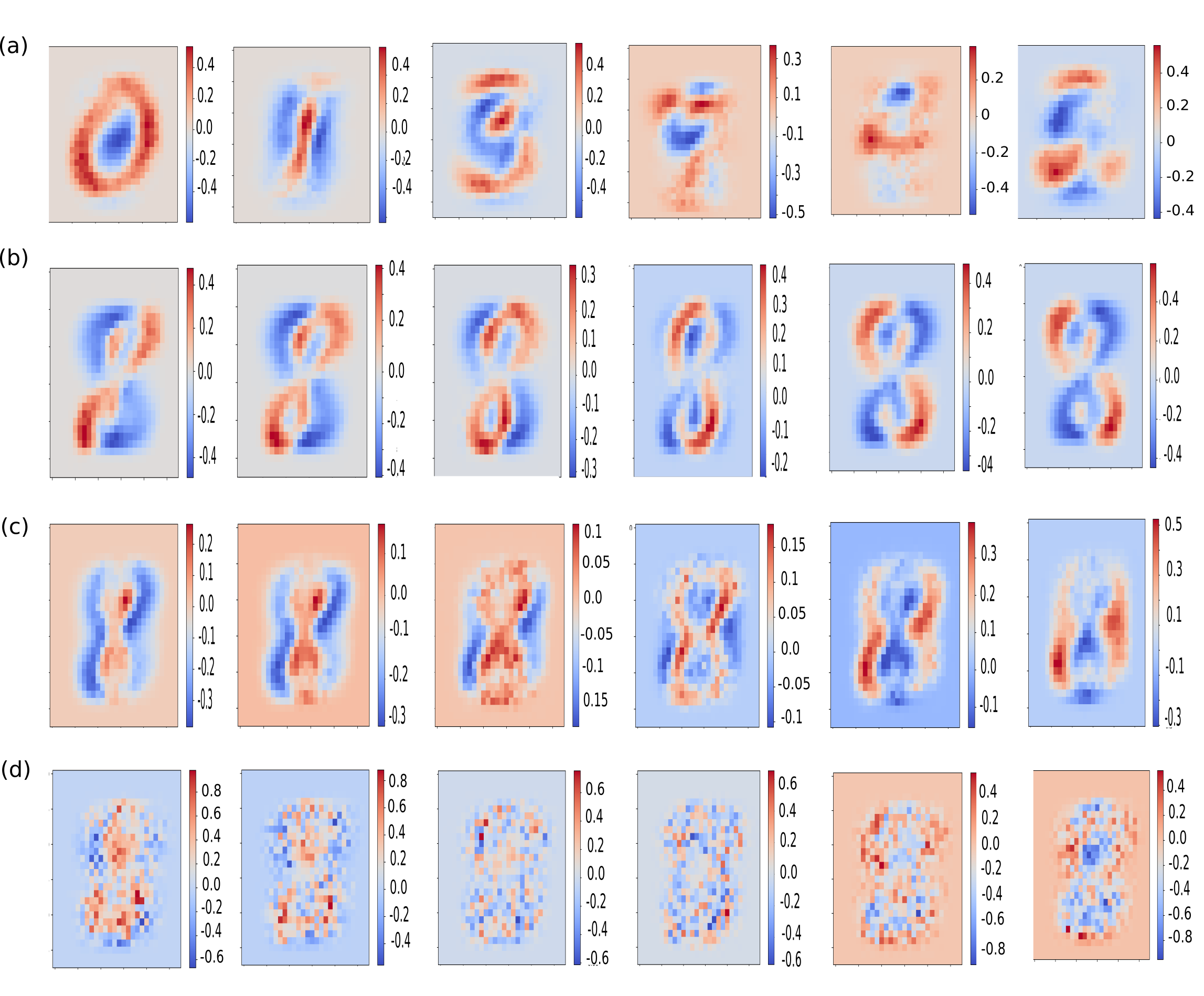
In order to further study the correctness of our causal attributions, we evaluated our algorithm on data where explicit causal relations are known. In particular, if a dimension in the representation represents unique generative factors, they can be regarded as causal factors for data. To this end, we train a conditional (Kingma et al. 2014) -VAE (Higgins et al. 2016) on MNIST data to obtain disentangled representations which represent unique generative factors. The latent variables were modeled as 10 discrete variables (for each digit class) (which were conditioned on while training the VAE) and 10 continuous variables (for variations in the digit such as rotation and scaling) . was set to . Upon training, the generative decoder was taken and and (Defn. 4.2) were computed for each decoded pixel and intervened latent variables . In case of continuous latents, along with each , is also intervened on (ensuring ) to maintain consistency with the generative process. Since we have access to a probabilistic model through the VAE, the interventional expectations were calculated directly via Eqn 2. For each , the baseline was computed as in Sec 4.1. For the binary s, we took as the baseline. (More details are in Appendix A.6.2.)
Fig 5a corresponds to ACE of (from left to right) on each pixel of the decoded image (as output). The results indicate that is positively causal () for pixels at spatial locations which correspond to the digit. This agrees with the causal structure (by construction of VAE, causes the digit image). Figs 5b, c and d correspond respectively to ACE of with intervened values () increased from -3.0 to 3.0 (, so deviations) and . The latents and seem to control the rotation and scaling of the digit 8 respectively. All other ’s behave similar to the plots for , with no discernable causal effect on the decoded image. These observations are consistent with visual inspection on the decoded images after intervening on the latent space. More results with similar trends are reported in Appendix A.6.3.
6 Conclusions
This work presented a new causal perspective to neural network attribution. The presented approach views a neural network as an SCM, and introduces an appropriate definition, as well as a mechanism to compute, Average Causal Effect (ACE) effectively in neural networks. The work also presents a strategy to efficiently compute ACE for high-dimensional data, as well as extensions of the methodology to RNNs. The experiments on synthetic and real-world data show significant promise of the methodology to elicit causal effect of input on output data in a neural network. Future work will include extending to other neural network architectures (such as ConvNets) as well as studying the impact of other baselines on the proposed method’s performance. Importantly, we believe this work can encourage viewing a neural network model from a causal lens, and answering further causal questions such as: which counterfactual questions might be asked and answered in a neural network causal model, can a causal chain exist in a neural network, are predictions made by neural networks causal, and so on.
Acknowledgements
We are grateful to the Ministry of Human Resource Development, India; Department of Science and Technology, India; as well as Honeywell India for the financial support of this project through the UAY program. We thank the anonymous reviewers for their valuable feedback that helped improve the presentation of this work.
References
- Abadi et al. (2016) Abadi, M., Barham, P., Chen, J., Chen, Z., Davis, A., Dean, J., Devin, M., Ghemawat, S., Irving, G., Isard, M., et al. Tensorflow: A system for large-scale machine learning. In OSDI, volume 16, pp. 265–283, 2016.
- Alvarez-Melis & Jaakkola (2017) Alvarez-Melis, D. and Jaakkola, T. S. A causal framework for explaining the predictions of black-box sequence-to-sequence models. arXiv preprint arXiv:1707.01943, 2017.
- Alvarez-Melis & Jaakkola (2018) Alvarez-Melis, D. and Jaakkola, T. S. Towards robust interpretability with self-explaining neural networks. arXiv preprint arXiv:1806.07538, 2018.
- Bach et al. (2015) Bach, S., Binder, A., Montavon, G., Klauschen, F., Müller, K.-R., and Samek, W. On pixel-wise explanations for non-linear classifier decisions by layer-wise relevance propagation. PloS one, 10(7):e0130140, 2015.
- Bongers et al. (2016) Bongers, S., Peters, J., Schölkopf, B., and Mooij, J. M. Structural causal models: Cycles, marginalizations, exogenous reparametrizations and reductions. arXiv preprint arXiv:1611.06221, 2016.
- Christopher (2016) Christopher, M. B. PATTERN RECOGNITION AND MACHINE LEARNING. Springer-Verlag New York, 2016.
- Claeskens et al. (2008) Claeskens, G., Hjort, N. L., et al. Model selection and model averaging. Cambridge Books, 2008.
- Daniusis et al. (2010) Daniusis, P., Janzing, D., Mooij, J., Zscheischler, J., Steudel, B., Zhang, K., and Schölkopf, B. Inferring deterministic causal relations. pp. 143–150, 01 2010.
- Deng et al. (2014) Deng, L., Yu, D., et al. Deep learning: methods and applications. Foundations and Trends® in Signal Processing, 7(3–4):197–387, 2014.
- Dheeru & Karra Taniskidou (2017) Dheeru, D. and Karra Taniskidou, E. UCI machine learning repository, 2017. URL http://archive.ics.uci.edu/ml.
- Eberhardt (2007) Eberhardt, F. Causation and intervention. Unpublished doctoral dissertation, Carnegie Mellon University, 2007.
- Frosst & Hinton (2017) Frosst, N. and Hinton, G. Distilling a neural network into a soft decision tree. arXiv preprint arXiv:1711.09784, 2017.
- Geiger et al. (1990) Geiger, D., Verma, T., and Pearl, J. Identifying independence in bayesian networks. Networks, 20(5):507–534, 1990.
- Gilmer et al. (2017) Gilmer, J., Schoenholz, S. S., Riley, P. F., Vinyals, O., and Dahl, G. E. Neural message passing for quantum chemistry. arXiv preprint arXiv:1704.01212, 2017.
- Higgins et al. (2016) Higgins, I., Matthey, L., Pal, A., Burgess, C., Glorot, X., Botvinick, M., Mohamed, S., and Lerchner, A. beta-vae: Learning basic visual concepts with a constrained variational framework. 2016.
- Hochreiter & Schmidhuber (1997) Hochreiter, S. and Schmidhuber, J. Long short-term memory. Neural computation, 9(8):1735–1780, 1997.
- Hoyer et al. (2009) Hoyer, P. O., Janzing, D., Mooij, J. M., Peters, J., and Schölkopf, B. Nonlinear causal discovery with additive noise models. In Advances in neural information processing systems, pp. 689–696, 2009.
- Hyttinen et al. (2013) Hyttinen, A., Eberhardt, F., and Hoyer, P. O. Experiment selection for causal discovery. The Journal of Machine Learning Research, 14(1):3041–3071, 2013.
- Kiiveri et al. (1984) Kiiveri, H., Speed, T. P., and Carlin, J. B. Recursive causal models. Journal of the australian Mathematical Society, 36(1):30–52, 1984.
- Kindermans et al. (2017) Kindermans, P.-J., Hooker, S., Adebayo, J., Alber, M., Schütt, K. T., Dähne, S., Erhan, D., and Kim, B. The (un) reliability of saliency methods. arXiv preprint arXiv:1711.00867, 2017.
- Kingma et al. (2014) Kingma, D. P., Mohamed, S., Rezende, D. J., and Welling, M. Semi-supervised learning with deep generative models. In Advances in neural information processing systems, pp. 3581–3589, 2014.
- Kocaoglu et al. (2017) Kocaoglu, M., Snyder, C., Dimakis, A. G., and Vishwanath, S. Causalgan: Learning causal implicit generative models with adversarial training. arXiv preprint arXiv:1709.02023, 2017.
- Letham et al. (2015) Letham, B., Rudin, C., McCormick, T. H., Madigan, D., et al. Interpretable classifiers using rules and bayesian analysis: Building a better stroke prediction model. The Annals of Applied Statistics, 9(3):1350–1371, 2015.
- Li et al. (2018) Li, O., Liu, H., Chen, C., and Rudin, C. Deep learning for case-based reasoning through prototypes: A neural network that explains its predictions. In Thirty-Second AAAI Conference on Artificial Intelligence, 2018.
- Montavon et al. (2017) Montavon, G., Lapuschkin, S., Binder, A., Samek, W., and Müller, K.-R. Explaining nonlinear classification decisions with deep taylor decomposition. Pattern Recognition, 65:211–222, 2017.
- Pearl (2009) Pearl, J. Causality. Cambridge university press, 2009.
- Pearl (2012) Pearl, J. The do-calculus revisited. arXiv preprint arXiv:1210.4852, 2012.
- Peters et al. (2017) Peters, J., Janzing, D., and Schölkopf, B. Elements of causal inference: foundations and learning algorithms. MIT press, 2017.
- Ribeiro et al. (2016) Ribeiro, M. T., Singh, S., and Guestrin, C. Why should i trust you?: Explaining the predictions of any classifier. In Proceedings of the 22nd ACM SIGKDD International Conference on Knowledge Discovery and Data Mining, pp. 1135–1144. ACM, 2016.
- Sadowski et al. (2014) Sadowski, P. J., Whiteson, D., and Baldi, P. Searching for higgs boson decay modes with deep learning. In Advances in Neural Information Processing Systems, pp. 2393–2401, 2014.
- Selvaraju et al. (2016) Selvaraju, R. R., Das, A., Vedantam, R., Cogswell, M., Parikh, D., and Batra, D. Grad-cam: Why did you say that? arXiv preprint arXiv:1611.07450, 2016.
- Shrikumar et al. (2017) Shrikumar, A., Greenside, P., and Kundaje, A. Learning important features through propagating activation differences. arXiv preprint arXiv:1704.02685, 2017.
- Simonyan et al. (2013) Simonyan, K., Vedaldi, A., and Zisserman, A. Deep inside convolutional networks: Visualising image classification models and saliency maps. arXiv preprint arXiv:1312.6034, 2013.
- Smilkov et al. (2017) Smilkov, D., Thorat, N., Kim, B., Viégas, F., and Wattenberg, M. Smoothgrad: removing noise by adding noise. arXiv preprint arXiv:1706.03825, 2017.
- Sundararajan et al. (2017) Sundararajan, M., Taly, A., and Yan, Q. Axiomatic attribution for deep networks. arXiv preprint arXiv:1703.01365, 2017.
- Team (2017) Team, P. C. Pytorch: Tensors and dynamic neural networks in python with strong gpu acceleration, 2017.
- Yosinski et al. (2015) Yosinski, J., Clune, J., Nguyen, A., Fuchs, T., and Lipson, H. Understanding neural networks through deep visualization. arXiv preprint arXiv:1506.06579, 2015.
- Zeiler & Fergus (2014) Zeiler, M. D. and Fergus, R. Visualizing and understanding convolutional networks. In European conference on computer vision, pp. 818–833. Springer, 2014.
- Zhou & Troyanskaya (2015) Zhou, J. and Troyanskaya, O. G. Predicting effects of noncoding variants with deep learning–based sequence model. Nature methods, 12(10):931, 2015.
Appendix A Appendix
A.1 Causality Preliminaries
In this section, we review some of the basic definitions in causality that may help understand this work.
Structural Causal Models (SCMs) (Pearl 2009) provide a rigorous definition of cause-effect relations between different random variables. Exogenous variables (noise) are the only source of stochasticity in an SCM, with the endogenous variables (observables) deterministically fixed via functions over the exogenous and other endogenous variables.
Definition A.1.
(Structural Causal Models). A Structural Causal Model is a 4-tuple where, (i) is a finite set of endogenous variables, usually the observable random variables in the system; (ii) is a finite set of exogenous variables, usually treated as unobserved or noise variables; (iii) is a set of functions , where n refers to the cardinality of the set . These functions define causal mechanisms, such that . The set is a subset of and . We do not consider feedback causal models here; (iv) defines a probability distribution over . It is not necessary for every node in an SCM to have a unique/shared noise. Deterministic causal systems have been considered in literature (Daniusis et al. 2010).
An SCM can be trivially represented by a directed graphical model , where the vertices represent the endogenous variables (each vertex corresponds to an observable ). We will use random variables and vertices interchangeably henceforth. The edges denote the causal mechanisms . Concretely, if then , there exists a directed edge from the vertex corresponding to to the vertex corresponding to . The vertex is called the parent vertex while the vertex is referred to as the child vertex. Such a graph is called a causal Bayesian network. The distribution of every vertex in a causal Bayesian network depends only upon its parent vertices (local Markov property) (Kiiveri et al. 1984).
A path is defined as a sequence of unique vertices with edges between each consecutive vertex and . A collider is defined with respect to a path as a vertex which has a structure. (The direction of the arrows imply the direction of the edges along the path.) d-separation is a well-studied property of graphical models (Pearl 2009; Geiger et al. 1990) that is often used to decipher conditional independences between random variables that admit a probability distribution faithful to the graphical model.
Proposition 4.
(Pearl 2009) Two random variables and are said to be conditionally independent given a set of random variables if they are d-separated in the corresponding graphical model .
Definition A.2.
(d-separation). Two vertices and are said to be d-separated if all paths connecting the two vertices are “blocked” by a set of random variables .
A path is said to be “blocked” if either (i) there exists a collider that is not in , or, (ii) there exists a non-collider along the path. is the set of all vertices which exhibit a directed path to any vertex . A directed path from vertex to is a path such that there is no incoming edge to and no outgoing edge from .
The operator (Definition 4.1)(Pearl 2009; Pearl 2012) is used to identify causal effects from a given SCM or causal Bayesian network. Although similar in appearance to the conditional expectation , refers to the expectation of the random variable taken over its interventional distribution .
Definition A.3.
(Average Causal Effect). The Average Causal Effect (ACE) of a binary random variable on another random variable is commonly defined as .
Formally, a causal Bayesian network induces a joint distribution over its vertices . Performing interventions on random variables are analogous to surgically removing incoming edges to their corresponding vertices in the network . This is because the value of the random variables now depend on the nature of the intervention caused by the “external doer” and not the inherent causal structure of the system. The interventional joint distribution over the vertices of would be . Notice that in , the factorization of the interventional joint distribution ignores the intervened random variables . In an SCM , performing a operation is the same as an intervened SCM , where the causal mechanism for variable x, is replaced by the constant function . is obtained from the set by replacing all the instances of random variable in the arguments of the causal functions by .
A.2 More on Prior Work
Existing methods for attribution can broadly be categorized into gradient-based methods and local regression-based methods.
As stated in Sections 1 and 2 (main paper), in the former approach, gradients of a function are not ideal indicators of an input feature’s influence on the output. Partial derivatives of a continuous function are also functions over the same domain (the subscript denotes the partial derivative with respect to the input feature). The attribution value of the feature which is derived from would in turn be biased by the values of other input features. For instance, consider a simple function , . The respective partial derivatives are and . Consider a points . and . This implies that for output , had a stronger influence than . But in reality has a stronger contribution towards than . Gradients are thus viable candidates for the question “How much would perturbing a particular input affect the output?”, but not for determining which input influenced a particular output neuron.
Besides, perturbations and gradients can be viewed as capturing the Individual Causal Effect (ICE) of input neuron with values on output .
| (5) |
In Equation 5, denotes conditioning the input neurons other than to the input training instance values. The Expectation operator for is over the unobservable noise which is equal to the learned neural function itself, i.e., , where the baseline is for some . Evidently, inter-feature interactions can conceal the real importance of input feature in this computation, when only the ICE is analyzed.
The latter approach of “interpretable” regression is highly prone to artifacts as regression primarily maps correlations rather than causation. Regression of an output variable (the neural network output) on a set of input features is akin to calculating , given input features. However, true causal effects of on are discerned via , as in (Pearl 2009). The only way regressing on a particular input feature would give is if all the backdoor variables are controlled and a weighted average according to the distribution of these backdoor variables is taken (Pearl 2009). Thus, causal statements made from regressing on all input variables (say, the weights of a linear approximator to a deep network) would be far from the true picture.
A.3 Proofs
A.3.1 Proof of Proposition 1
Proof.
In a feedforward neural network, each layer neurons can be written as functions of neurons in its previous layer, i.e. . The input layer can be assumed to be functions of independent noise variables such that and . This structure in the random variables, neurons in the network, can be equivalently expressed by a SCM . ∎
A.3.2 Proof of Corollary 1.1
Proof.
All notations are consistent with their definitions in Proposition 1. Starting with each neuron in the output layer , the corresponding causal function can be substituted as . This can also be written as . refers to the causal function of neuron in layer . Similarly, refers to neuron in layer . Proceeding recursively layer by layer, we obtain modified functions such that, . The causal mechanisms set of the reduced SCM M’ would be { and ∎
A.3.3 Proof of Proposition 2
Proof.
Let be the causally sufficient SCM for a given SCM . Let be the corresponding causal bayesian network. Presence of dependency between input features in neural network implies the existence of common exogenous parent vertices in the graph . All the paths from one input neuron to another in graph either passes through an exogenous variable or a vertex corresponding to an output neuron. The output neurons are colliders and the intervention on , surgically removes all incoming edges to (refer to Section A.1). As all the paths from to every other input neuron are “blocked”, from Definition A.2, the intervened input neuron is d-seperated from all other input neurons. ∎
A.3.4 Proof of Proposition 3
Proof.
In the reduced SCM for the recurrent function , if the values of all other input neurons at different timesteps are controlled (fixed), transforms according to . Let’s assume depends on via a one-to-one mapping. Note, if there exists a one-to-one mapping between and , then the conditional entropy would be , thus maximizing the mutual information between the two random variables. So, we limit the lookback to only those timesteps that register a one-to-one mapping with .
The probability of in an infinitesimal volume is given by,
| (7) |
By change of variables
| (8) |
Now, and are volumes and hence are positive constants. exists in the training data and hence . Similarly, . Thus, if evaluated using Equation 8 is zero, there is a contradiction. Hence, the assumption that depends on via a one-to-one mapping is incorrect. . would be optimal for a particular input sequence and output . is taken as the for the entire dataset, to prevent re-computation for every new input sequence.
A.4 Algorithms/Pseudocode
A.4.1 Algorithm for Phase I in Feedforward Networks
Algorithm 1 outputs an array of size with interventional expectations of an output neuron given different interventions () on . The user input parameter decides how many evenly spaced values are desired. The accuracy of the learned polynomial functions in Phase II depends on the size of .
Consider training points, and input neurons in a feedforward network. Usually, to avoid memorization by the network. Computations are performed on-the-fly via a single pass through the computational graph in frameworks such as Tensorflow (Abadi et al. 2016) and PyTorch(Team 2017). If one single pass over the computational graph is considered unit of computation, the computational complexity of Phase I (Algorithm 1) would be O(). Compare this to the computational complexity of O() for calculating the interventional expectations naively. For every perturbation of neuron , we would require atleast forward passes on the network to estimate .
A.4.2 Algorithm for Phase I in Recurrent networks
See Algorithm 2. The input training data is arranged in a tensor of size .
A.4.3 Algorithm for Phase II
See Algorithm 3.
A.5 Scaling to Large Data
In this section we follow the same notations as defined in Section 4 in the main text. Evaluating the interventional expectations using Eqn 4 involves calculating the Hessian. This is a costly operation. For a system with input features it takes about backward passes along the computational graph. Several domains involve a large number of input features. Such a large regime would render Equation 4 inefficient. Note however that we never explicitly require the Hessian, just the term . In this section, we propose an efficient methodology to compute the interventional expectations for high-dimensional data.
We begin with computing , where is the input vector. Consider the eigendecomposition of , where is the eigenvector and the corresponding eigenvalue. Let . Performing a Taylor series expansion of around , we get:
Adding the equations:
Rather:
| (9) |
Equation 9 calculates the second order directional derivative along . Since ( and refer to the & entry of respectively), . Thus, the second order term in Eqn 4 can be calculated by three forward passes on the computational graph with inputs , where is the matrix with s as columns and is taken to be very small (). Although eigendecomposition is also compute-intensive, the availability of efficient procedures allowed us to get results significantly faster than exact calculations (0.04s for the approximation v/s 3.04s per computation for experiments on MNIST dataset with a deep neural network of 4 hidden layers).

A.6 More on Experiments and Results
A.6.1 Generation of Synthetic Dataset
We used the following procedure for generating the synthetic dataset used for experiments (Section 5.2):
- •
Sample individual sequences uniformly of length between . We used . Let refer to the sequence value at length .
- •
Sample .
- •
With probability either (a) sample and label such sequences class or (b) sample and label such sequences class .
A.6.2 Calculation of the interventional expectations in Section 5.4
From the generative model of the VAE we have access to . Each pixel is modelled as a Bernoulli random variable with parameter , being the continous latents and being the class-specific binary variables . Interventional expectations required for calculated ACEs are calculated via Equation 2.
For continuous latents:
From the generative model prior , we know that each is independently distributed according to , so the intervention does not change the distribution of the other variables. However, the multinouli distribution over the s forces all the other . Thus, the above expression can be simply computed via Monte Carlo integration as follows: , where samples are drawn.
For discrete latents: there are two cases depending on the intervention value .
Case 1:
As before, the multinoulli distribution over the s restricts all the other . Thus, the above expression can be simply computed via Monte Carlo integration as follows:
, where samples are drawn.
Case 2:
Now, as , the distribution over all the other . Thus, the above expression can be simply computed via Monte Carlo Integration as follows, , where samples are drawn.
A.6.3 Additional Results: Visualizing Causal Effect
In continuation to results in Section 5.4, we present additional results here. We fix the class part of the latent and sample a random vector z from . Then we intervene on one of the dimensions of z and pass the latent through the decoder. We intervene with values in the range -3 to 3. This is repeated for every dimension. When the decoded images are sorted based on the value of intervention, we are able to see the effect of rotation in dimension and the effect of scaling in dimension . Other dimensions show no effect, as shown in Figure 7.

Figure 8 shows causal attributions of the continuous latents (defined in Section 5.4) for the decoded image for different class-specific latents (). In all the cases and capture rotation and scaling of the digit respectively. like all the other s showed no discernable causal effect. We also show causal attributions of these latents for digits 0, 2 and 3 in Figure 8 to 10.


