Modeling atom-atom interactions at low energy by Jost-Kohn potentials

In the absence of any bound state, $\log g(z)$ becomes regular for ${\rm Re}[z]>0$ for $g(0)\neq 0$ and continuous for ${\rm Re}[z]\geq 0$, its imaginary part being equal to the phase shift as given by $\eta(k)={\rm Im}\left[\log g(z)\right]$. Now, one can represent $\log g(z)$ in ${\rm Re}[z]\geq 0$ in terms of phase shift $\eta(k)$ by Poisson’s integral

Suppose, $\eta(k)$ admits an effective range expansion

where it is assumed that $a_{s}<0$. Using the relation $\tan^{-1}x=(i/2)\log[(1-ix)/(1+ix)]$, one can express $\eta(k)$ in the form

where $a=\frac{2}{r_{0}}\left[1+\sqrt{1-\frac{2r_{0}}{a_{s}}}\right]$, $b=\frac{2}{r_{0}}\left[-1+\sqrt{1-\frac{2r_{0}}{a_{s}}}\right]$. Substituting Eq.(19) in Eq.(17), one obtains

where $\lambda=\frac{\left(b-a\right)}{2a}$ is a small parameter ($|\lambda|<1$). Expanding the potential $U(r)$ in polynomial form

each of the terms $U_{m}(r)$ can be calculated by inverse Laplace transform of $\Phi_{m}(z)$ as discussed above. The detailed derivation is given in the appendix-A. The resulting series can be expressed in a compact form, giving an explicit expression

for negative $a_{s}$. From here onward, for the sake of simplicity, we consider $r_{0}$ as the unit of length, and the quantity $E_{0}=\hbar^{2}/(2\mu r_{0}^{2})$ as the unit of energy, unless otherwise specified.

For positive scattering length, the potential may support bound states. The binding energies of the bound states given by the zeros $\xi_{i}$ of $g(z)$ in ${\rm Re}[z]>0$ lie on the real axis for $z$-plane. Therefore, in presence of bound states, the function $g(z)$ needs to be modified. Suppose, there exists $m$ bound states. Then the modified $g(z)$ reads as

which is non-zero for ${\rm Re}[z]>0$ and follow the same asymptotic properties of $g(z)$. The modified Eq.(17) have the form of

Let the binding energy of $i$ th bound state energy be

In deriving a potential that can support only one bound state and give positive $a_{s}$, Jost and Kohn first calculated an auxiliary potential $V_{+}(r)$ which may yield the same low energy scattering cross section but no bound state. The Jost function corresponding to $V_{+}(r)$ is assumed to have the form

which obviously does not have a proper zero for the bound state. $V_{+}(x)$ is derived by iteration as above. This is expressed in terms of the three parameters which are $r_{0}$, $a_{s}$ and a dimensionless parameter $\Lambda$ related to the binding energy $E_{b}=-\hbar^{2}\kappa^{2}/2\mu$ of the bound state. The detailed method of derivation is discussed in appendix B. Explicitly,

where, $x=\frac{r}{r_{0}}$, $\alpha=\sqrt{1-\frac{2r_{0}}{a_{s}}}$, $\beta=1+\alpha$ and

is a parameter with $-1<\Lambda<1$ and determined by $\kappa$.

Though $V_{+}(r)$ does not support any bound state, it explicitly depends on the parameter $\kappa$ which determines binding energy $E_{b}$ of a bound state that is supported by an ”equivalent” potential, say $V_{b}(r)$. The $S$-matrix for $V_{+}(r)$ is $S=e^{2i\tilde{\eta}}=\tilde{f}(k)/\tilde{f}(-k)$ where $\tilde{\eta}$ is the phase shift and $\tilde{f}(k)$ is given by Eq.(26). It is easy to deduce that in the limit $\kappa\rightarrow\infty$, $\tilde{\eta}$ becomes independent of $\kappa$ and so the phase shift in the low energy limit will be determined only by $a_{s}$ and $r_{0}$. On the other hand, for small $\kappa$, $\tilde{\eta}$ will depend on all the three parameters $a_{s}$, $r_{0}$ and $\kappa$. As given by Eq.(23), we have

where $\eta(k)$ corresponds to $V_{b}(r)$ and is assumed to have an effective range expansion in terms of $a_{s}$ and $r_{0}$ as in Eq. (18) but for $a_{s}>0$. The expression (29) shows that, for $\kappa\neq 0$ and $k\rightarrow 0$, $\tilde{\eta}=\eta-\pi$. So, both the potentials $V_{+}(r)$ and $V_{b}(r)$ will yield the same $s$-wave scattering cross section at low energy. The question here is how $\kappa$ affects the effective range expansion.

From Eq.(29), we obtain

Assuming that $\kappa a_{s}>2$ or $\kappa a_{s}<2$ and $k\ll\kappa$ (for low energy scattering), we have $1\gg\mid\frac{1-r_{0}\kappa}{\frac{2}{\kappa a_{s}}-1}\mid\frac{k^{2}}{\kappa^{2}}$. After binomial expansion in Eq.(30), up to the second order in $k/\kappa$, we get

where

where $\bar{r}_{0}$ is the modified range. From this formula, it is clear that $\bar{r}_{0}$ is negative but $\bar{a}_{s}>0$ for $\kappa r_{0}<\!<1$ and $\kappa a_{s}>2$. On the other hand, $\bar{a}_{s}<0$ for $\kappa a_{s}<2$. So, for $\kappa a_{s}<\!<1$, $\bar{r}_{0}$ may vary from positive to negative values as $\kappa r_{0}$ changes from small ($<\!<1$) to large values ($>\!>1$). The negativity of $\bar{r}_{0}$ may be interpreted as resulting from the breakdown of the standard effective range expansion due to the proximity of a zero-energy resonance as we describe in the next subsection. In the standard effective range expansion bethe; LandauLifshitz_QM as in Eq.(18), it is assumed that $kr_{0}<<1$ and $r_{0}>0$. For $V_{+}(r)$, we have found that the numerically calculated $a_{s}$ and $r_{0}$ agree quite well with the chosen values of $a_{s}$ and $r_{0}$ used to construct $V_{+}(r)$ if $\kappa r_{0}>\!>4$. We find that the numerical calculated values of $\bar{a_{s}}$ and $\bar{r_{0}}$ deviate substantially from the chosen $a_{s}$ and $r_{0}$ if $\kappa r_{0}<<1$.

In this subsection we first calculate the scattering phase shift and cross section as a function of collision energy $E$ or wave number $k$ for Jost-Kohn potentials. Zero-energy resonance occurs when $\eta(0)=\pi/2$, that is, the $s$-wave phase shift at $k=0$ is $\pi/2$. This happens if $f(0)=0$, physically this implies that the potential is about to support a bound state at an energy given by $f(k\neq 0)=0$ if the potential is slightly modified. This follows from the fact that there exists no bound state at zero energy for $s$ wave unlike that at higher partial waves. A bound state for $s$-wave can exist only at finite energy, in which case $f(0)\neq 0$ and $\eta(0)=\pi$ schieff_book.

From the effective range expansion, it follows that for $a_{s}\rightarrow-\infty$, we have $\eta(0)\rightarrow\pi/2$. Since $V_{-}(r)$ is derived based solely on the effective range expansion, one would expect that numerically calculated phase shift for $V_{-}(r)$ should reproduce this result. In fact, the calculated phase shift as plotted in Fig.1 shows this expected behavior.

The Jost function corresponding to the potential $V_{+}(r)$ is given by $\tilde{f}(k)$ of Eq.(26). One can notice that $\tilde{f}(0)\neq 0$ if $\kappa\neq 0$. In this case, in the limit $k\rightarrow 0$, the $S$-matrix $S(k)=\tilde{f}(k)/\tilde{f}(-k)$ approaches identity and so the the phase shift $\eta(0)\rightarrow\pi$. On the other hand, for $\kappa=0$, $a_{s}=\infty$, we have $S(k\rightarrow 0)\rightarrow-1$. The expression Eq.(31) shows that for $\kappa a_{s}<2$, $k\rightarrow 0$, $a_{s}\rightarrow\infty$ with $ka_{s}>>1$, we have $\cot\bar{\eta}(k)\rightarrow 0_{+}$ implying that $\eta(k\rightarrow 0)=\pi/2$. Therefore the system exhibits zero-energy resonance.

In Fig.2. we have plotted the $s$-wave scattering cross sections $\sigma_{0}(E)$ as a function of dimensionless energy $E/E_{0}$ in the resonance limit. Consequently $\sigma_{0}(E)$, shows a divergent signature in the limit $E\rightarrow 0$ as in Fig.2. From the inset of Fig.2, it is clear that the phase shift goes to $+\frac{\pi}{2}$ as $\kappa\rightarrow 0$. In this context, it is worth mentioning that both the potentials $V_{+}(r)$ and $V_{-}(r)$ reduce to the same analytical form which is of Potsch-Teller potential in the limits $\Lambda\rightarrow-1$ (or $\kappa\rightarrow 0$) and $a_{s}\rightarrow\pm\infty$ deb:injmp:2016, signifying zero-energy resonance. It is worth mentioning that the same from of Pöschl-Teller potential has been used earlier for quantum Monte Carlo simulation of many-body physics of an ultracold Fermi gas of atoms carlson:prl:2003; forbes:pra86:2012; li:pra84:2011; morris:pra81:2010; schonenberg:pra:95:2017.

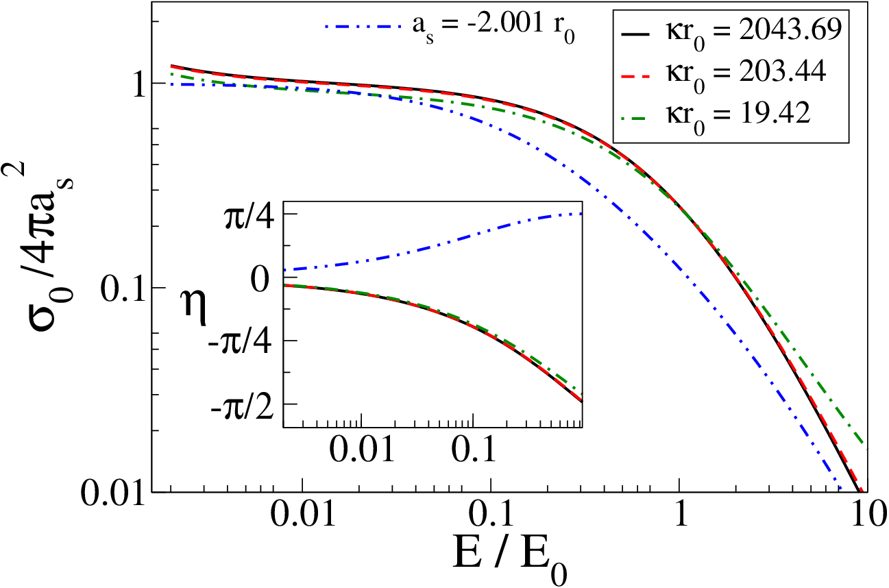
Jost-Kohn potentials do not explicitly reduce to a delta-function like zero-range contact potential in the limit $r_{0}\rightarrow 0$. The derivation of $V_{+}(r)$ makes use of the assumption $a_{s}>2r_{0}$. Here we numerically verify whether the Jost-Kohn potentials reproduce the known results of weak interaction regime (small $|a_{s}|$) in the limit $r_{0}\rightarrow 0$. In Fig.3. we show the variation of scattering cross section as a function of energy, for large $\kappa$. Here, the quantity $\frac{\sigma_{0}}{4\pi a_{s}^{2}}$ nearly equals to unity at very low energy limit. We have verified this limit for different values of $\kappa$ and scattering lengths. The inset of Fig.3 exhibits the behavior of the phase shift in the limit $E\rightarrow 0$. We notice that $\eta(E\rightarrow 0)\propto\pm\sqrt{E}$, where $+(-)$ corresponds to negative(positive) $a_{s}$. This low energy behavior of $\eta(E)$ is consistent with that for a contact or weak interaction potential.

Having shown that the Jost-Kohn potentials can describe the standard low energy scattering properties of a pair of ultracold atoms in free space, we now discuss whether these potentials are good enough to model the interaction between a pair of trapped atoms. There exists an exact solution for a pair of ultracold atoms interacting via a regularized contact potential in a 3D isotropic harmonic oscillator butsch:foundphys:1998. Several theoretical studies studies have shown that this exact solution is good enough so long as $|a_{s}|$ is much smaller than the characteristic length scale or more specifically the size of the ground state of the isotropic harmonic oscillator. In a previous study physscrpt:partha, it has been demonstrated that the bound state solutions of a pair of ultracold atoms interacting via Jost-Kohn potentials in an isotropic harmonic oscillator can qualitatively reproduce the results of Ref.butsch:foundphys:1998 when $r_{0}$ is much smaller than the harmonic oscillator length scale provided $a_{s}$ is small enough. Also, for a quasi-one dimensional trap, Jost-Kohn potentials are shown to agree qualitatively with the results of a contact interaction only when $r_{0}$ is much smaller than the length scale of the transverse 2D harmonic oscillator and small $a_{s}$ physscrpt:partha.

Here we discuss to what extent and under what physical conditions it may be possible to describe Feshbach-resonant interactions between ultracold atoms by Jost-Kohn potentials. Feshbach resonance is a multichannel scattering problem where a quasi-bound state supported by one or multiple closed channels is made degenerate or quasi-degenerate with the bare scattering state of at least one open channel by means of an external magnetic or optical field. As a consequence, a Feshbach resonance occurs due to an admixture of bound and continuum states leading to a dressed continuum which can also be dealt with Fano’s method fano1961; debandgsa:jpb:2009. If there is only one open channel, then the physical $S$-matrix derived upon elimination of all the closed channels corresponds to the open channel only. If the experimentally determined phase shift corresponding to this effective single-channel physical $S$-matrix element admits an effective range expansion with the effective range $r_{f}$ (we use different notation for the effective range of the Feshbach resonance to distinguish it from $r_{0}$ that corresponds to Jost-Kohn potentials) then the method of Jost and Kohn will be definitely applicable to this effective single-channel problem. The pertinent question here is how to reduce a multi-channel scattering problem into an effective single-channel one describable by the Jost-Kohn potentials.

In the current literature on magnetic Feshbach resonances chin:rmp2010; sresonance of ultracold atoms, the resonances are mainly categorized into two types depending on the width of the resonance: narrow or closed-channel dominated and broad or open-channel dominated ones. The width of a Feshbach resonance is quantified by the dimensionless strength parameter defined by $s_{res}=\frac{\delta\mu\Delta}{\bar{E}}\frac{a_{bg}}{\bar{a}}$, where $\delta\mu$ is the difference between the magnetic moments of the bare quasi-bound state and the two separated atoms, $a_{bg}$ is the background scattering length and $\Delta$ in unit of magnetic field strength is the width of the resonance. For a potential behaving asymptotically as $-\frac{C_{6}}{r^{6}}$, with $C_{6}$ being the van der Waals’ coefficient, Gribakin and Flambaum vanderwaal defined a length scale called the mean scattering length $\bar{a}=\frac{2\pi}{\Gamma(1/4)^{2}}\Big(\frac{2\mu C_{6}}{\hbar^{2}}\Big)^{1/4}$, and corresponding energy scale $\bar{E}=\frac{\hbar^{2}}{2\mu\bar{a}^{2}}$. A narrow or closed-channel-dominated resonance occurs when $s_{res}<1$ while for a broad or entrance-channel-dominated resonance, $s_{res}>1$. Gao gao and Flambaum et al.Flambaum have defined an effective range $R_{e}$ for asymptotic van der Waals potential by $R_{e}\approx\left(\frac{\Gamma(\frac{1}{4})^{4}}{6\pi^{2}}\right)\bar{a}\left[1-2\left(\frac{\bar{a}}{a_{s}}\right)+2\left(\frac{\bar{a}}{a_{s}}\right)^{2}\right]$. The $r_{f}$-dependence of a narrow Feshbach resonance has been shown to be quite different from that of a broad Feshbach resonance effrange. It has been further demonstrated, both theoretically efferangetheo and experimentally range; pra:2013:hulet that $r_{f}$ near a narrow Feshbach resonance may become quite large, negative and magnetic field-dependent. The experimental observation range shows that near the narrow Feshbach resonance ($B_{0}=58.9$G) of ³⁹K the effective range sharply changes with scattering length (or magnetic field) and the effective range is found to be large negative in the vicinity of this Feshbach resonance. For the case of ⁶Li NFR near 543.3G, similar results are found pra:2013:hulet. In contrast, $r_{f}$ near a broad Feshbach resonance is usually positive, small and close to $R_{e}$. In the case of an intermediate-range Feshabch resonance ($s_{res}\sim 1$), quite interesting field-dependence of $r_{f}$ has been experimentally demonstrated pra:2013:hulet. From the analysis made in subsection 3.2, we understand that the effective range of the resonant interaction with $a_{s}>0$ may be controlled by the parameter $\kappa$ of the potential $V_{+}$.

In the case of $a_{s}<0$, the model Jost-Kohn potential $V_{-}(r)$ has only two parameters, $r_{0}$ and $a_{s}$ and so it is straightforward to model a Feshbach resonance by using these two parameters as fitting parameters provided the Feshbach-resonance phase shift $\eta_{r}$ admits an effective range expansion with $r_{f}>0$. Then $r_{0}=r_{f}$ and the Feshbach-resonant scattering length is the same as in $V_{-}(r)$. In fact, even in the case of a narrow Feshbach resonance, $r_{f}$ is found to be positive in the regime of negative $a_{s}$ in many of ultracold atomic species pra:2013:hulet. However, in the case $a_{s}>0$, we need three parameters, the third parameter $\kappa$ determines the binding energy of the bound state of an equivalent potential. In order to discuss how to model Feshbach-resonant interaction with $V_{+}(r)$, it may be instructive to recall the salient features of two-channel model of Feshbach resonances twochannel which has found considerable applications in modeling magnetic Feshbach resonances (MFR) of ultracold atoms chin:rmp2010.

In the two-channel model, the lower channel is open and the upper channel is closed, meaning that the asymptotic collision energy is above the threshold of the open channel but below the threshold of the closed channel. The closed channel is assumed to support a bound state $\psi_{c}(r)$ with binding energy $E_{c}$. There is a coupling $W(r)$ between the two channels. The $S$-matrix for the open channel is given by

where $\eta_{bg}$ is a non-resonant background phase shift, $E_{{\rm shift}}$ is a shift of the closed-channel bound state due to its coupling with the bare scattering state of the open channel and $\Gamma_{f}$ is the Feshbach resonance width defined by $\Gamma_{f}=2\pi\mid\int\psi_{c}(r)W(r)\psi_{E}(r)dr\mid^{2}$ where $\psi_{E}(r)$ is the bare scattering state of the open channel at collision energy $E$. The resonance phase shift $\eta_{r}$ is given by

where $\tilde{E}_{c}=E_{c}+E_{{\rm shift}}$. The total phase shift is $\eta=\eta_{bg}+\eta_{r}$. Therefore, we have

Considering $\eta_{bg}$ being small, one may approximate $\cot\eta_{bg}\simeq-1/ka_{bg}$ where $a_{bg}$ is the background scattering length. This approximation is particularly good for a narrow resonance. At low energy, $\Gamma_{f}$ may be proportional to $k$, because the energy-normalized scattering wave function asymptotically behaves as $\psi_{E}(r)\sim\sqrt{k}r$. This will happen if $W(r)$ is most prominent beyond the range of the open channel potential. Under these conditions, we may write $k\cot\eta_{r}\simeq-\frac{1}{a_{r}}+\frac{1}{2}r_{r}k^{2}$ where $\frac{1}{a_{r}}=-\lim_{k\rightarrow 0}\frac{2k\tilde{E}_{c}}{\hbar\Gamma_{f}}$ and $r_{r}=-\lim_{k\rightarrow 0}\frac{2\hbar k}{\mu\Gamma_{f}}$. In an MFR, the energy $\tilde{E}_{c}$ of the quasi-bound state is magnetically tuned across the threshold of the open channel. The resonant scattering length $a_{r}$ is negative (positive) if $\tilde{E}_{c}$ is positive (negative). The resonance at zero energy occurs when $\tilde{E}_{c}$ is zero, in which case $a_{r}\rightarrow\infty$.

From Eq. (36), we can obtain $k\cot\eta\simeq-1/\bar{a_{s}}+(1/2)r_{f}k^{2}$ where $\frac{1}{\bar{a_{s}}}=\frac{1}{a_{r}}\left(1-\frac{a_{bg}}{a_{r}}\right)$ and

Close to resonance, $|a_{bg}|<\!<|a_{r}|$. Writing $\Gamma_{f}\simeq kG$, where $G$ is a constant, we note that the parameter $r_{r}$ is inversely proportional to $G$. Therefore, $r_{r}$ will be large for small $G$ or for a narrow resonance. Let us now assume that $a_{bg}>0$ and consider the case $a_{r}>0$. For a broad resonance, usually $r_{f}$ is positive and small. This means that, for a broad resonance $\kappa$ should be large and we may set $\bar{r}_{0}\simeq r_{0}=r_{f}$. In the case of far-off resonance, we may set $\kappa\rightarrow\infty$ and $r_{0}=R_{e}$. In the case of a narrow resonance, the parameter $\kappa$ can be used to control the deviation of $r_{f}$ from $R_{e}$. For a magnetic field very close to resonant magnetic field at which $a_{s}\rightarrow+\infty$, we can safely assume that $\kappa a_{s}>\!>2$ so that $\bar{a}_{s}\simeq a_{s}$ as follows from Eq.(32). Then the value of $\kappa$ can be set by equating Eq.(33) with the experimentally observed $r_{f}$ assuming $r_{0}=R_{e}$. The negative effective range can be mimicked by making $\kappa r_{0}<4$. In the universality regime chin:rmp2010, $\bar{a}_{s}=1/\kappa$, implying that for $a_{bg}>0$ and $a_{bg}<<a_{r}$, $\Gamma_{f}\propto k\kappa$ which will happen if the bound state behaves as $e^{-kr}$. This means that inter-channel coupling should predominantly occur in the asymptotic limit of the bound state. Then $r_{r}\sim 1/\kappa$, therefore in the limit $\kappa\rightarrow 0$, $r_{r}$ will be large and the effective range $r_{f}$ as given by Eq.(37) will be large negative indicating the breakdown of the effective range expansion. Universality regime is found to occur mostly in broad Feshbach resonances for which it has been shown that nonlinear energy dependence of the phase shift even very close to zero energy becomes important, suggesting that effective range expansion may fail at the universality regime efferangetheo.

References

- (1) R. Jost and W. Kohn, Phys. Rev. 84, 977 (1952).
- (2) R. Jost and W. Kohn, Dan. Mat. Fys. Medd 27, no. 9 (1953).
- (3) E. Braaten, M. Kusunoki and D. Zhang, Ann. Phys. 323, 1770-1815 (2008).
- (4) I. Bloch, J. Dalibard, and W. Zwerger, Rev. Mod. Phys.80, 885 (2008).
- (5) C. Chin, R. Grimm, E. Tiesinga, and P. S. Julienne,Rev. Mod. Phys. 82, 1225 (2010).
- (6) T. Köhler, K. Goral and P. S. Julienne, Rev. Mod. Phys. 78, 1311-1361 (2006).
- (7) T. D. Lee, K. Huang and C. N. Yang, Phys. Rev. 106, 1135 (1957).
- (8) K. Huang, Statistical Mechanics (John Wiley & Sons, 1987), Second edition.
- (9) C. L. Blackley , P. S. Julienne and J. M. Hutson,Phys. Rev. A 89 042701 (2014).
- (10) E. L. Hazlett, Y. Zhang, R. W. Stites and K.M.O’Hara,Phys. Rev. Lett. 108, 045304 (2012).
- (11) P. Dyke, S. E. Pollack, and R. G. Hulet, Phys. Rev. A 88, 023625 (2013).
- (12) S. Roy, M. Landini, A. Trenkwalder, G. Semeghini, G. Spagnolli, A. Simoni, M. Fattori, M. Inguscio, and G. Modugno, Phys. Rev. Lett. 111, 053202 (2013).
- (13) C. Ji, D. R. Phillips and L. Platter, Ann. Phys. 327, 1803-1824 (2012).
- (14) C. H. Greene, P. Giannakeas and J. Pérez-Ríos, Rev. Mod. Phys.89, 035006 (2017).
- (15) A. Kievsky, M. Gattobigio, Phys. Rev. A 92, 062715 (2015).
- (16) C. L. Blackley, C. R. L. Sueur, J. M. Hutson, D. J. McCarron, M. P. Köppinger, H. W. Cho, D. L. Jenkin and S. L. Cornish Phys. Rev. A 87, 033611 (2013).
- (17) E. L. Bolda, E. Tiesinga and P. S. Julienne, Phys. Rev. A 66, 013403 (2002).
- (18) I. M. Gel’fand and B. M. Levitan, Dokl. Akad. Nauk. USSR 77, 557-560 (1951); I. M. Gel’fand and B. M. Levitan, Izv. Akad. Nauk. SSRser. Math. 15, 309-360 (1951).
- (19) L. I. Schiff, Quantum Mechanics (Tata McGraw-Hill, 1968), Third edition.
- (20) L. D. Landau and E. M. Lifshitz, Quantum Mechanics (Pergamon Press, 1965), Vol. 3, Second edition.
- (21) S. Zöllner, H. D. Meyer and P. Schmelcher, Phys. Rev. A 74, 053612 (2006);Phys. Rev. A 75, 043608 (2007); H. Wu and J. E. Thomas, Phys. Rev. A 86, 063625 (2012).
- (22) P. I. Schneider, S. Grishkevich and A. Saenz, Phys. Rev. A 80, 013404 (2009).
- (23) A. D. Lange, K. Pilch, A. Prantner, F. Ferlaino, B. Engeser, H.-C. Nägerl, R. Grimm, and C. Chin, Phys. Rev. A 79, 013622 (2009).
- (24) V. V. Flambaum, F. G. Gribakin and C. Harabati, Phys. Rev. A 59 1998 (1999).
- (25) H. Veksler, S. Fishman and W. Ketterle Phys. Rev. A 90, 023620 (2014).
- (26) T. Köhler, T. Gasenzer, P. S. Julienne and K. Burnett,Phys. Rev. Lett. 91, 230401 (2003).
- (27) B. Gao J. Phys. B: At. Mol. Opt. Phys. 36, 2111 (2003).
- (28) B. Gao Phys. Rev. A 64 010701 (R) (2001).
- (29) V. Bargmann, Rev. of Mod. Phys. 21, 488 (1949).
- (30) R. B. Johnson, J. Chem. Phys. 67, 4086 (1977).
- (31) H. A. Bethe, Phys. Rev. 76, 38 (1949).
- (32) B. Deb, Int. J. Mod. Phys. B 30, 1650036 (2016).
- (33) J. Carlson, S. Y. Chang, V. R. Pandharipande and K. E. Schmidt, Phys. Rev. Lett. 91, 050401 (2003).
- (34) M. M. Forbes, S. Gandolfi and A. Gezerlis, Phys. Rev. A 86, 053603 (2012).
- (35) X. li, J. Kolorenč and L. Mitas, Phys. Rev. A 84, 023615 (2011).
- (36) A. J. Morris, P. L. Ríos and R. J. Needs, Phys. Rev. A 81, 033619 (2010).
- (37) L. M. Schonenberg and G. J. Conduit Phys. Rev. A 95, 013633 (2017).
- (38) T. Busch, B. G. Englert, K. Rzazewski and M. Wilkens,Foundation of Physics 28, 549 (1998).
- (39) E. Tiesinga, C. J. Williams, F. H. Miles and P. S. Julienne, Phys. Rev. A 61, 063416 (2000).
- (40) P. Goswami and B. Deb, Phys. Scr. 91 , 085401 (2016).
- (41) U. Fano, Phys. Rev. 124, 1866 (1961).
- (42) B. Deb and G. S. Agarwal, J. Phys. B: At. Mol. Opt. Phys. 42 , 215203 (2009).
- (43) G. F. Gribakin and V. V. Flambaum, Phys. Rev. A 48, 546 (1993).
- (44) B. Gao Phys. Rev. A 58 4222 (1998).
- (45) T. L. Ho, X. Cui and W. Li, Phys. Rev. Lett. 108, 250401 (2012).